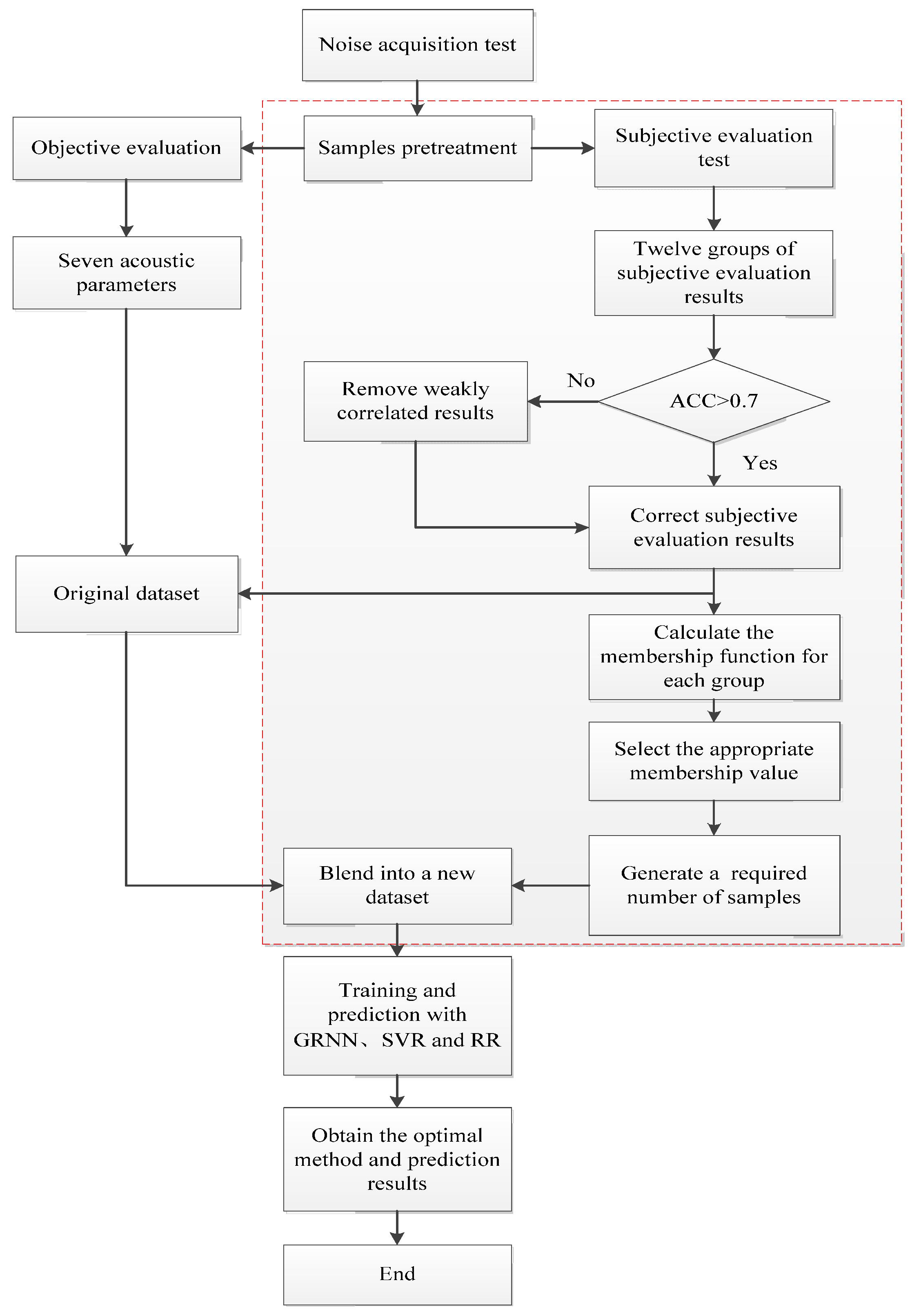
Article

Small Sample Sound Quality Prediction Method of Hy-Vo Chain Transmission System Based on Fuzzy Generation

School of Mechanical and Aerospace Engineering, Jilin University, Changchun 130022, China
*
Author to whom correspondence should be addressed.
Appl. Sci. 2024, 14(8), 3147; https://doi.org/10.3390/app14083147
Submission received: 14 March 2024 / Revised: 5 April 2024 / Accepted: 6 April 2024 / Published: 9 April 2024
(This article belongs to the Section Acoustics and Vibrations)

Abstract

:
To improve the noise comfort of the whole machine, it is necessary to establish the sound quality prediction model of the Hy-Vo chain transmission system. Compared with the silent chain transmission system, the Hy-Vo chain transmission system normally operates at a lower speed and cannot have too much load at the limit speed. It is difficult to obtain a sufficient quantity of high-quality noise samples because there are few different working conditions. For small sample sound quality prediction, we use a sample enhancement method called fuzzy generation based on fuzzy mathematics. Firstly, audio samples of the Hy-Vo chain transmission system are collected through noise tests. Secondly, the processed samples are evaluated objectively and subjectively. After a correlation test of the subjective evaluation results, correct subjective evaluation scores of each noise sample are obtained. With the help of fuzzy generation, we can obtain a sufficient number of new samples. By mixing the original samples with the generated samples, a new dataset is created. Through using a general regression neural network (GRNN), support vector regression (SVR) model, and ridge regression (RR) method, the sound quality of the Hy-Vo chain transmission system can be predicted. Different from prediction results under the original dataset, using the fuzzy generation method can not only significantly reduce the prediction error of the model but also improve stability.

1. Introduction

Hy-Vo chain is an advanced product in the field of chain drive, and it is different from an ordinary chain because of its variable pith characteristics. Thanks to this variable pitch characteristic, it reduces the polygon effect in the transmission process and has a more unique noise performance [1,2]. Nowadays, it has been proved that noise has great damage to human mental and physical health, and people generally pay more attention to the quality of machine noise [3]. As a widely used transmission system, the Hy-Vo chain system is a decisive factor in the noise performance of the whole machine, so its sound quality needs to be studied.
Previous studies on Hy-Vo chain noise only focus on sound pressure level (SPL), and a single parameter cannot fully measure the human ear perception of noise. To evaluate the sound quality of the Hy-Vo chain system, more acoustic parameters need to be introduced [4]. In the field of sound quality research, many researchers use loudness, sharpness, roughness, fluctuation, tonality, articulation index (AI), and other parameters as objective evaluation. After the subjective evaluation score test, an appropriate regression model and method are selected to fit the nonlinear relationship between the parameters and human ear perception [5,6]. In the early stage, the method of multiple linear regression was used to predict the sound quality, but there is often serious multicollinearity among the parameters, resulting in poor accuracy of the model. Recently, more researchers have adopted deep learning-related methods to make predictions, such as back propagation neural networks, convolutional neural networks, and extreme gradient boosting [7,8,9]. When the quantity and quality of samples are sufficient, the deep learning method can well fit the nonlinear relationship between inputs and outputs. However, under the condition of small sample learning, the prediction model often has a serious overfitting phenomenon, and the fitting degree and accuracy of the model are very low.
To solve the problem of predicting sound quality in small samples, we use a method called fuzzy generation based on fuzzy mathematics to increase the number of samples [10,11]. The fuzzy generation method comes from a fuzzy phenomenon in the subjective evaluation of sound quality, that is, people’s auditory perception of the same audio will be different. Therefore, the subjective evaluation result is uncertain, and we can measure it by defining fuzzy mapping and constructing membership functions. A generation interval can be defined by selecting the appropriate membership value, and we can obtain a sufficient number of new samples by randomly perturbing the sample label values in this interval. After the generated samples are mixed with the original dataset into a new large dataset, three methods of general regression neural network (GRNN), support vector regression (SVR), and ridge regression (RR) are used to train on the old and new datasets, respectively. The prediction results show that using the fuzzy generation method can greatly reduce errors and improve the fitting degree of the models. In addition, the GRNN model performs best. It not only greatly improves the prediction accuracy, model fit, and stability under large membership values but also has a better ability to resist data noise interference than the SVR model and RR model under small membership values. Figure 1 shows the flow chart of the small sample sound quality prediction method for the Hy-Vo chain system, and the part enclosed by the red line is the fuzzy generation method.

2. Acquisition and Processing of Noise Samples

2.1. Noise Test

To get close to the real working scene of the Hy-Vo chain system, a noise test is carried out in the indoor reverberation environment. The Hy-Vo chain sample and equipment required for the test are shown in Figure 2. For the chain sample, the pitch is 9.525 mm, the number of links is 84, the chain form is 4 × 3, the drive sprocket tooth number is 35, and the driven sprocket tooth number is 37. The measurement microphone (UMIK-1 from miniDSP technology company, Hong Kong, China) is positioned at the same height as the center of the drive sprocket to collect noise. We select two noise acquisition positions: one is at 0.5 m from the center of the drive sprocket and the other one is at 1 m from that. In the test, loads are 500 N and 750 N, respectively, and the speed range is 500–6000 rpm. The noise acquisition process is as follows: we first place the measuring microphone at the position of 0.5 m, start the motor, and adjust the speed to 500 rpm. After the load is set to 500 N, the noise audio is recorded using Adobe Audition software 2022 in a stable running state. The sampling frequency is 48,000 Hz, and the sampling time is greater than 30 s. After the first audio sample is obtained, the load is increased to 750 N and the second audio sample can be taken. The measuring microphone is moved to the position of 1 m, keeping the height and direction of the microphone unchanged, and we collect the third audio sample at the load of 750 N. The load is reset to 500 N and the fourth audio sample is recorded. Each time the speed increases by 500 rpm and the above collection process is repeated, we can finally get 12 × 2 × 2 = 48 noise samples. For each noise sample, Adobe Audition software 2022 is used to randomly intercept consecutive 5 s clips for subsequent study.
Figure 3 compares the time-domain waveform between the Hy-Vo chain and the silent chain. Under the same load condition, the noise energy of the Hy-Vo chain system at 1500 rpm is slightly higher than that of the silent chain system, but at 3000 rpm, the noise of the Hy-Vo chain system is significantly stronger than that of the silent chain system. We know that the noise performance of the Hy-Vo chain system is worse at high speed, so it is different from the sound quality of the silent chain system. Therefore, it is necessary and meaningful to study the sound quality of the Hy-Vo chain system.

2.2. Subjective Evaluation

As presented in Table 1, we evaluate the sound quality according to the degree of discomfort and adopt the equal interval direct one-dimensional evaluation method [12]. There are five levels of discomfort in Table 1, where 0 indicates extreme discomfort with the highest level of noise annoyance and 10 indicates no discomfort. Each of the three remaining discomfort levels contains three scores, each score representing the discomfort degree at the same level.
We selected twelve healthy testers (ten males and two females) with no ear problems, all testers were between the ages of 20 and 30 and had driving experience. The subjective evaluation test was conducted in an indoor environment with a maximum sound pressure level of no more than 20 dB. The tester sits on the chair with earphones and the audio is played by Groove software (version number: 11.2402.6.0). The process of the evaluation test is as follows: The tester randomly played the first audio, which was repeated three times and then stopped. After listening to the first noise sample, the tester had a hearing perception of the sample. Based on Table 1, the tester could give the final score of the sample. The score was recorded in an Excel spreadsheet, and the tester randomly switched to the next audio until all 48 noise samples were completely evaluated. The twelve testers took turns participating in the evaluation test, and the subjective evaluation results are illustrated in Figure 4.
In Figure 4, the horizontal line in the middle of each box line represents the median score, and the upper and lower boundaries of the box line represent the upper and lower quartiles. Taking the median score as a benchmark, we can find that the score generally presents a step-down trend with the increase in rotational speed. When the rotational speed is in the range of 500–1500 rpm, the score is reduced with the increase of the rotational speed. When the rotational speed is in the range of 2000–3000 rpm, compared with the value at 1500 rpm, the score is steady and unchanging. When the rotational speed is at the range of 3500–4500 rpm, compared with the value at 3000 rpm, the score drops and remains stable at 3500 rpm and 4000 rpm and then drops again at 4500 rpm. The score of 5000–6000 rpm has the same downward trend as the 3500–4500 rpm. According to the above analysis, we can know the relationship between the noise performance of the Hy-Vo chain system and the rotational speed. At low speeds, the noise performance is negatively correlated with the rotational speed. At middle speed, the chain system is in optimum working condition and the noise performance remains relatively stable. At high speeds, the noise performance is not good and continues to deteriorate with the increase in rotational speed.
For the same sample, twelve testers must have relatively consistent feelings. From Figure 4, we use box line length to evaluate the score fluctuation at the same speed. Obviously, the score fluctuates least at low speed, less at medium speed, and more at high speed. To test whether the subjective evaluation score of each sample is reasonable, we calculate the correlation coefficient R between the twelve groups of evaluation results. The equation of R is as follows:
R = i = 1 n ( x i x ¯ ) ( y i y ¯ ) i = 1 n ( x i x ¯ ) 2 i = 1 n ( y i y ¯ ) 2
where xi and yi represent the corresponding elements of the two variables and x ¯ and y ¯ represent the average value of the corresponding variables. The strength of correlation is positively correlated with the absolute value of R.
Based on Equation (1), the values of R between the twelve testers are computed in Figure 5. When the value of R is greater than 0.7, the two are strongly correlated and vice versa. In Figure 5, P1 to P12 represents the number of testers, and the strength of the correlation is also described by the depth of color. It is easy to see that only the correlation values of P5–P6 and P5–P11 are less than 0.7, and the rest are strongly correlated. To make a final screening decision, the average correlation coefficient (ACC) of each tester needs to be calculated, as shown in Table 2.
As can be seen from Table 2, the ACC of P12 is 0.897 at the highest, and the lowest ACC is 0.737 for P5. ACCs of the twelve testers are all more than 0.7, indicating that the scores of all samples are reasonable. Then, we can compute the average score of each sample as its final subjective evaluation, and the calculation results are shown in Table 3.

2.3. Objective Evaluation

Different from previous studies of the Hy-Vo chain system, we use seven acoustic parameters to study the noise performance, and the parameters are as follows: SPL, A-weighted sound pressure level (A-SPL), loudness, sharpness, roughness, fluctuation, and AI. Because the Audio Toolbox in MATLAB is a handy tool for calculating acoustic parameters, we can use it to calculate the seven objective parameters for 48 noise samples, as shown in Figure 6. After the above subjective and objective evaluation, an original dataset for sound quality prediction can be obtained, and the dataset is listed in Table 4.

3. Fuzzy Generation

Fuzzy mathematics is a mathematical tool for dealing with uncertain information, which is developed on the basis of fuzzy set theory. Different from traditional probability theory and statistics, fuzzy mathematics does not deal with the uncertainty of randomness but with the uncertainty caused by various reasons (such as fuzziness, incompleteness, imprecision, etc.). In view of the fuzzy phenomenon in the research, the introduction of fuzzy mathematics theory can deal with the shortcomings of traditional mathematics in dealing with fuzzy problems [13,14,15,16].
In the study of sound quality, we found a fuzzy problem in that researchers only chose the mean of subjective evaluation scores as the final score. However, here is the fact that all scores for the same sample should be reasonable after the correlation test. There are subtle differences in how people perceive the same sample, and this uncertainty is reflected in the study of sound quality. Therefore, there is a certain fuzziness in the final results of subjective evaluation. In our study, 12 scores are given for one noise sample, and the minimum and maximum values constitute the maximum reasonable interval of subjective evaluation scores. To improve the universality of subjective evaluation results, we use a method of fuzzy generation to obtain a sufficient number of sample points within the maximum reasonable interval. The functions of the fuzzy generation method are as follows: it can not only be used to measure the ambiguity of each sample point in the interval but also to determine the interval range and way of sample generation.
For the same sample, we set up a fuzzy interval of sample generation with the mean score as the kernel and the extreme score as a boundary. The fuzzy intervals of all samples are shown in Table 5, and then we define a mapping on this fuzzy interval as follows:
H : V [ 0 , 1 ] v H ( v )
where V is the value field [0, 10], H is the fuzzy interval of V, and H(v) is the membership function.
Based on the kernel and boundary points of the fuzzy interval, we can construct the membership function as follows:
H ( v d ) 0 d u = 1 0 k u H ( v d ) = 1 u k ( u d )
H ( v d ) 0 d l = 1 0 k l H ( v d ) = 1 k l ( d l )
where k is the kernel value, l is the minimum value, u is the maximum value, d is a random value, and H(vd) is the membership of d.
According to Equations (3) and (4), we calculate the membership functions of all samples, as shown in Figure 7.
In Figure 7, when the score is as large as the kernel value, the membership reaches a maximum of 1. When the score gradually moves away from the kernel value from both sides, the membership gradually decreases until it reaches a minimum value of 0 at the two boundary points. In theory, the closer the generated sample point is to the kernel value, the closer it is to the real test result. However, if there is only a small disturbance around the kernel value, there is suspicion of data leakage. Therefore, it is most important to study how to choose a suitable membership value.
The details of the fuzzy generation method we use in this paper are as follows: For the membership function of all samples, we select five membership values (0.9, 0.7, 0.5, 0.3, 0.1) from the largest to the smallest to divide the sample generation interval. Generally speaking, the smaller the membership value is, the larger the interval is, and the more noise the generated new sample contains. For each sample, we use MATLAB 2021a to randomly generate two new samples on each interval. Finally, we can obtain 96 new samples for each membership value. After mixing with the original dataset, we can obtain five new datasets with 144 samples. We use these five datasets to train the subsequent sound quality prediction model, which can test the effectiveness of the fuzzy generation method and analyze the influence of membership value on the model.
It should be pointed out that when using fuzzy generation, the key is to construct or select the appropriate membership function for the original sample. Membership value selection should also be reasonable: a too-large value may lead to data leakage and a too-small value will introduce too much noise and damage the performance of the model. Also, the way to generate new samples is not limited to random generation.

4. Sound Quality Prediction

4.1. Modeling

To test the effect of fuzzy generation, different models need to be trained on the old and new datasets to compare the advantages and disadvantages of prediction results, and the ratio of training set to test set is 4:1. At the same time, the influence of five membership values on prediction results can be compared. Furthermore, when training with the original dataset, it can be regarded as the case where the membership value is equal to 1. In this paper, we set up different prediction models based on three methods: general regression neural network (GRNN), support vector regression (SVR) model, and ridge regression (RR). The reason why these three methods are chosen is that they all have their specific advantages: GRNN has a strong nonlinear mapping ability and can handle the nonlinear relationship between acoustic parameters and evaluation scores. SVR is more concerned with determining the best-fit line and limiting the error to a certain threshold. There is often a certain correlation between objective acoustic parameters, and RR can handle the strong correlation between variables to improve the stability of the model.
(1)
GRNN model
General regression neural network (GRNN) is a type of neural network based on radial basis function (RBF), which is mainly used for regression analysis and function approximation. Generally speaking, GRNN mainly has two biggest advantages, on the one hand, the structure is simple, including the input layer, mode layer, summation layer, and output layer. On the other hand, there is only one key parameter called the smoothing factor, a small smoothing factor will cause the network to overfit, while a large smoothing factor may cause the network to underfit [17,18,19].
To find the optimal smoothing factor, we choose to use the particle swarm optimization (PSO) algorithm. In this paper, the number of particles is set to 30 and the maximum number of iterations is set to 20. The optimization results of the smoothing factor are shown in the following Table 6.
(2)
SVR model
Support vector regression (SVR) is a regression version of support vector machines (SVM), but unlike SVM classification, where the goal is to find a hyperplane that maximizes the interval, SVR aims to find a hyperplane so that most of the data points fall within the tolerance range of this hyperplane. To perform nonlinear regression in high-dimensional space, SVR can use different kernel functions, such as linear kernel, polynomial kernel, RBF kernel, and sigmoid kernel. There are two key parameters c and g in SVR, c is called the regularization parameter and g is called the kernel parameter. The size of the c value determines the tolerance of the model to error, and the size of the g value determines the influence range of each training sample [20,21,22].
We establish an SVR model with the RBF kernel in this research and use PSO to obtain the best c value and best g value. The initial conditions of PSO are set: the number of particles is 30 and the maximum number of iterations is 20. The final optimization results are shown in Table 7.
(3)
RR model
Ridge regression (RR), also known as Tikhonov regularization, is a regularized version of linear regression. It solves the multicollinearity problem in linear regression by adding a regular term to the loss function, thereby improving the stability and predictive power of the model. RR has a parameter λ that controls the strength of the regularization, and when λ = 0, RR is an ordinary linear regression. As λ increases, the intensity of regularization increases and the complexity of the model decreases. Through cross-validation, we can find the best λ value that minimizes the cross-validation error [23,24,25,26]. In this paper, we use five-fold cross-validation to get the best λ value under different datasets, as shown in Table 8.

4.2. Comparison of Prediction Results

To evaluate the effect of the prediction model more directly, mean absolute percentage error (MAPE), coefficient of determination (R2), and residual predictive deviation (RPD) are used as evaluation indexes. Among the three evaluation indexes, MAPE is used to compare the prediction accuracy of the three models, R2 is used to represent the fitting degree of the three models, and RPD is used to measure the generalization ability and stability of the three models.
MAPE is a percentage that represents the average relative difference between the predicted error and the true value. A lower MAPE value indicates that the model’s predictions are more accurate. Based on MAPE, we can compute the prediction accuracy as follows:
M A P E = ( 1 n i = 1 n | y ^ i y i y i | ) × 100 %
A c c u r a c y = 1 M A P E
where n is the number of samples, y ^ i is the predicted value of the sample, and yi is the true value of the sample.
On the six datasets, we trained the three models with seven acoustic parameters as inputs and subjective evaluation scores as outputs, and the optimal parameters of each model are substituted by Table 6, Table 7 and Table 8 above. The comparison of prediction accuracy on the three models is shown in
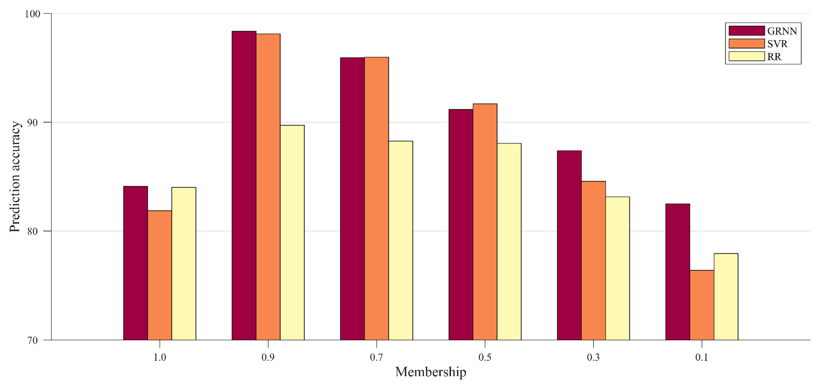
 Figure 8.
As can be seen from Figure 8, on the new data set generated by fuzzy generation, the prediction accuracy of the three models all showed a downward trend with the decrease of membership value. Among the three models, the GRNN model has more advantages than the other two models. Although the accuracy of the GRNN model decreases with the decrease in membership value, the decline trend is more uniform. When the membership value is less than 0.5, the advantages of the GRNN model are more prominent. For the SVR model, when the membership value is not less than 0.5, its prediction accuracy is close to the GRNN model, and sometimes even a little better. However, when the membership value is less than 0.5, the accuracy of the SVR model drops sharply. When the membership value is not less than 0.3, the prediction accuracy of the SVR model is obviously greater than that of the RR model, but when the membership value is a minimum of 0.1, the prediction accuracy of the SVR model is the lowest. For the RR model, the changing trend of its prediction accuracy is basically the same as the SVR model. Though the decline trend is slower, the RR model is always weaker than the SVR model when the membership value is not less than 0.3.
In Figure 8, compared with training on the original dataset (i.e., when the membership value is equal to 1), when the membership value is not less than 0.5, the use of the fuzzy generation method greatly improves the prediction accuracy of the models. When the membership value is 0.3, the accuracy of the GRNN model and the SVR model is still greater, but the RR model is no longer better. When the membership value is 0.1, the accuracy of the three models is worse than that trained under the original dataset, and the accuracy of the SVR model is the lowest. In general, the results show that rational use of fuzzy generation can improve the prediction accuracy of models. By comparing the prediction accuracy of the three models, it can be found that the GRNN model has the best performance, and it not only has high prediction accuracy when the membership value is large, but it also has strong resistance to large data noise when the membership value is small.
The values of R2 range from 0 to 1, the closer the value is to 1, the better the model fits. If the R2 value is close to 0, it means that the model is not explaining most of the variation in the data.
R 2 = 1 i = 1 n ( y i y ^ i ) 2 i = 1 n ( y i y ¯ ) 2
where n is the number of samples, y ^ i is the predicted value of the sample, yi is the true value of the sample, and y ¯ is the average of the predicted values.
The comparison of R2 on the three models is shown in
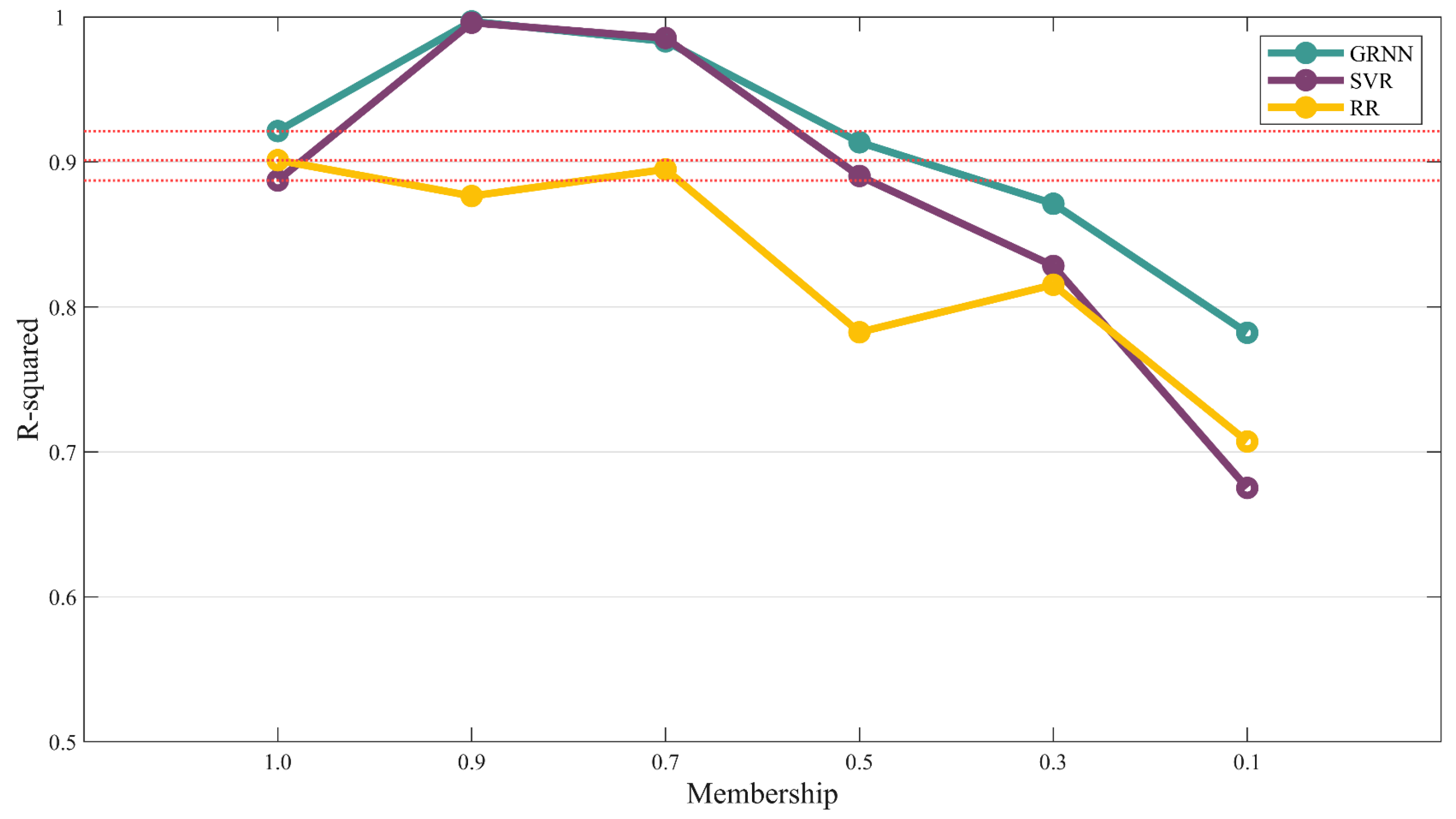
 Figure 9. Based on Figure 9, we can see that on the new dataset, the fitting degree of both the GRNN model and the SVR model is positively correlated with the membership value, and the GRNN model is better than the SVR model overall. For the RR model, the fitting degree fluctuates up and down as the membership value decreases. This phenomenon of R2 value fluctuation indicates that with the decrease in membership value, the degree of disturbance gradually increases, and the noise of data also increases. However, the specific form and distribution of the noise may be different every time, and the RR model cannot handle the influence of these noises well, resulting in the fluctuation of the R2 value. Compared with the membership value of 1, the fitting degrees of both the GRNN model and SVR model are obviously better when the membership value is 0.7 and 0.9. But when the membership value is less than 0.5, the fitting degree is worse. For the RR model, the fitting degree is lower for all membership values, indicating that the data noise introduced by fuzzy generation damages the performance of the model. By comparing the fitting degree of the three models, it can be found that when the membership degree is large, the fitting degree of the GRNN and SVR models is similar and far better than that of the RR model. When the membership value decreases gradually, it can be seen that the GRNN model has the strongest fitting ability.
A high RPD value means that the prediction error of the model is relatively small, indicating that the model has good consistency and stability under different datasets or conditions.
R P D = i = 1 n ( y i y ¯ ) 2 n 1 i = 1 n [ ( y ^ i y i ) ( y ^ y i ) ¯ ] 2 n 1
where n is the number of samples, y ^ i is the predicted value of the sample, yi is the true value of the sample, and y ¯ is the average of the predicted values.
The comparison of RPD on the three models is shown in 
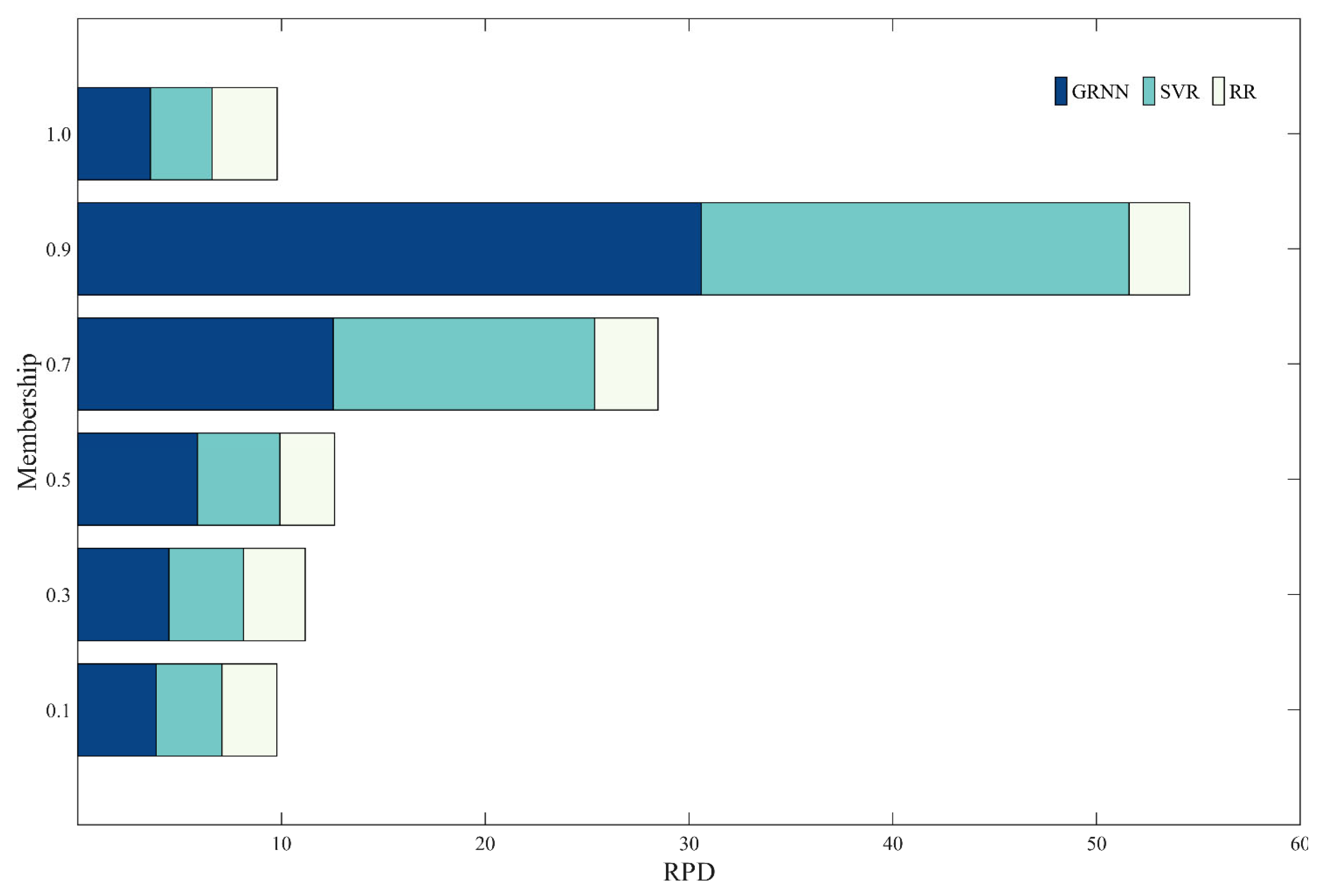
Figure 10. As can be seen from Figure 10, after the fuzzy generation method is used, the model stability of the GRNN model is the best, the SVR model is second, and the RR model is the worst. With the decrease in membership value, the RPD values of both the GRNN model and the SVR model show a decreasing trend, which indicates that the stability of the model becomes worse. For the RR model, the RPD value is not related to the size of the membership value, and the stability of the model remains basically unchanged at a low level. Compared with the membership value of 1, the stability of both the GRNN model and the SVR model is greatly improved by using the fuzzy generation method. Even when the membership value is at the minimum of 0.1, they still have a good performance. However, for the RR model, the use of the fuzzy generation method slightly reduces the stability of the model. By comparing the stability of the three models, the use of fuzzy generation can make GRNN and SVR models more stable, in which the GRNN model is stronger than the SVR, but both of them are significantly better than the RR model.

5. Conclusions

This paper presents a method for predicting the sound quality of the Hy-Vo chain transmission system in the case of small samples. The main conclusions are summarized as follows:
(1)
First of all, we conducted the noise acquisition test of the Hy-Vo chain transmission system under different working conditions. Secondly, we evaluated the processed noise samples subjectively and objectively. To solve the problem of small sample prediction, we found and made use of the fuzzy phenomenon in sound quality prediction, and then introduced fuzzy mathematics theory to use a sample generation method called fuzzy generation.
(2)
After using the fuzzy generation to expand the dataset, we used three different models to test the effect of this new method, namely, the GRNN model, the SVR model, and the RR model. On the new dataset, the prediction accuracy of all three models was significantly improved. The fitting degree and stability of both the GRNN model and the SVR model were higher than before when the membership degree was medium and high. Only the fitting degree and stability of the RR model did not get better or even worse for all membership values.
To sum up, fuzzy generation is an effective method for small sample sound quality prediction, which solves the problem of low model accuracy and easy overfitting in the case of small samples. Moreover, compared with the performance of different models, the GRNN model is more suitable for sound quality prediction of the Hy-Vo chain transmission system. Therefore, the sound quality prediction method based on fuzzy generation proposed in this paper not only provides a new idea for the research field of chain drive but also puts forward a novel and effective method for the related research of sound quality prediction. It should be pointed out that different types of chain drive systems have different noise characteristics, so the sound quality prediction model proposed in this paper cannot be applied directly. For a specific chain drive system, the process of establishing the sound quality prediction model is as follows: First of all, it is necessary to redesign the noise acquisition test and obtain a new noise sample set. Secondly, the acoustic parameters to be analyzed are selected and calculated, and the testers should be selected according to the application scenario. Then, the objective parameters and subjective evaluation results are analyzed and screened, and the data set for sound quality prediction can be obtained. Finally, the optimal sound quality prediction model is constructed and trained.

Author Contributions

Conceptualization, J.L.; Data curation, J.L.; Formal analysis, L.A.; Funding acquisition, Y.C.; Investigation, H.W.; Methodology, J.L. and L.A.; Project administration, Y.C.; Resources, Y.C.; Software, J.L.; Supervision, L.A.; Validation, J.L., L.A. and H.W.; Visualization, J.L.; Writing—original draft, J.L.; Writing—review and editing, J.L. and L.A. All authors have read and agreed to the published version of the manuscript.

Funding

This research was funded by [National Natural Science Foundation of China] grant number [51775222] and [Science and Technology Development Project of Jilin Province in China] grant number [20200401136GX]. And The APC was funded by [51775222].

Institutional Review Board Statement

Not applicable.

Informed Consent Statement

Not applicable.

Data Availability Statement

The raw data supporting the conclusions of this article will be made available by the authors on request.

Conflicts of Interest

The authors declare no conflicts of interest.

References

  1. Cheng, Y.B.; Gao, W.; Liu, H.; Zhang, J.Y.; Li, Y. Research on design method of Hy-Vo silent chain system for multi-phase transmission. Mech. Based Des. Struct. Mach. 2021, 49, 121–130. [Google Scholar] [CrossRef]
  2. Cheng, Y.B.; An, L.C.; Yin, S.B.; Wang, X.P. Multi-variation characteristic of dual phase Hy-Vo silent chain transmission system. Mech. Mach. Theory 2016, 103, 40–50. [Google Scholar] [CrossRef]
  3. Basner, M.; Babisch, W.; Davis, A.; Brink, M.; Clark, C.; Janssen, S.; Stansfeld, S. Auditory and non-auditory effects of noise on health. Lancet 2014, 383, 1325–1332. [Google Scholar] [CrossRef] [PubMed]
  4. Cheng, Y.; Wang, X.; Qi, H.; Li, L.; Fu, Z.; Wan, N. Noise Characteristics Test of Hy-Vo Silent Chain for Hybrid Vehicles. In Proceedings of the Joint International Information Technology, Mechanical and Electronic Engineering Conference (JIMEC), Xi’an, China, 4–5 October 2016. [Google Scholar]
  5. Kim, S.Y.; Ryu, S.C.; Jun, Y.D.; Kim, Y.C.; Oh, J.S. Methodology for Sound Quality Analysis of Motors for Automotive Interior Parts through Subjective Evaluation. Sensors 2022, 22, 6898. [Google Scholar] [CrossRef]
  6. Song, X.D.; Yang, W. Research on the Sound Quality Evaluation Method Based on Artificial Neural Network. Sci. Program. 2022, 2022, 8686785. [Google Scholar] [CrossRef]
  7. Chen, P.S.; Xu, L.Y.; Tang, Q.S.; Shang, L.L.; Liu, W. Research on prediction model of tractor sound quality based on genetic algorithm. Appl. Acoust. 2022, 185, 108411. [Google Scholar] [CrossRef]
  8. Wang, Y.Q.; Zhang, S.; Meng, D.J.; Zhang, L.J. Nonlinear overall annoyance level modeling and interior sound quality prediction for pure electric vehicle with extreme gradient boosting algorithm. Appl. Acoust. 2022, 195, 108857. [Google Scholar] [CrossRef]
  9. Ruan, P.L.; Zheng, X.; Qiu, Y.; Hao, Z.Y. A Binaural MFCC-CNN Sound Quality Model of High-Speed Train. Appl. Sci. 2022, 12, 12151. [Google Scholar] [CrossRef]
  10. Zhu, J.M.; Geng, Y.G.; Li, W.B.; Li, X.; He, Q.Z. Fuzzy Decision-Making Analysis of Quantitative Stock Selection in VR Industry Based on Random Forest Model. J. Funct. Spaces 2022, 2022, 7556229. [Google Scholar] [CrossRef]
  11. Khan, M.B.; Santos-Garcia, G.; Noor, M.A.; Soliman, M.S. Some new concepts related to fuzzy fractional calculus for up and down convex fuzzy-number valued functions and inequalities. Chaos Solitons Fractals 2022, 164, 112692. [Google Scholar] [CrossRef]
  12. Guski, R. Psychological methods for evaluating sound quality and assessing acoustic information. Acustica 1997, 83, 765–774. [Google Scholar]
  13. Gundogdu, F.K.; Kahraman, C. Spherical fuzzy sets and spherical fuzzy TOPSIS method. J. Intell. Fuzzy Syst. 2019, 36, 337–352. [Google Scholar] [CrossRef]
  14. Bustince, H.; Barrenechea, E.; Pagola, M.; Fernandez, J.; Xu, Z.; Bedregal, B.; Montero, J.; Hagras, H.; Herrera, F.; De Baets, B. A Historical Account of Types of Fuzzy Sets and Their Relationships. IEEE Trans. Fuzzy Syst. 2016, 24, 179–194. [Google Scholar] [CrossRef]
  15. Ruan, K.; Li, Y. Fuzzy mathematics model of the industrial design of human adaptive sports equipment. J. Intell. Fuzzy Syst. 2021, 40, 6103–6112. [Google Scholar] [CrossRef]
  16. Agayan, S.M.; Kamaev, D.A.; Bogoutdinov, S.R.; Aleksanyan, A.O.; Dzeranov, B.V. Time Series Analysis by Fuzzy Logic Methods. Algorithms 2023, 16, 238. [Google Scholar] [CrossRef]
  17. Vijayan, S.V.K.; Mohanta, H.; Pani, A.K. Adaptive non-linear soft sensor for quality monitoring in refineries using Just-in-Time Learning-Generalized regression neural network approach. Appl. Soft Comput. 2022, 119, 108546. [Google Scholar] [CrossRef]
  18. Yao, Q.H.; Wang, Y.; Yang, Y.X.; Yang, L. DOA estimation using GRNN for acoustic sensor arrays. Multidimens. Syst. Signal Process. 2023, 34, 575–594. [Google Scholar] [CrossRef]
  19. Zhu, Z.J.; Hong, Y.; Liang, Z. A Prediction Model for Top-Coal Drawing Capability in Steep Seams Based on PCA-GRNN. Geofluids 2022, 2022, 3590764. [Google Scholar] [CrossRef]
  20. Zhan, A.Y.; Du, F.; Chen, Z.Z.; Yin, G.X.; Wang, M.; Zhang, Y.J. A traffic flow forecasting method based on the GA-SVR. J. High Speed Netw. 2022, 28, 97–106. [Google Scholar] [CrossRef]
  21. Shi, M.L.; Lv, L.Y.; Guo, Z.G.; Sun, W.; Song, X.G.; Li, H.Y. High-Low Level Support Vector Regression Prediction Approach (HL-SVR) for Data Modeling with Input Parameters of Unequal Sample Sizes. Int. J. Comput. Methods 2021, 18, 2150029. [Google Scholar] [CrossRef]
  22. Shangguan, L.X.; Yin, Y.F.; Zhang, Q.T.; Liu, Q.; Xie, W.; Dong, Z.J. Icing Time Prediction Model of Pavement Based on an Improved SVR Model with Response Surface Approach. Appl. Sci. 2022, 12, 8109. [Google Scholar] [CrossRef]
  23. Zhang, R.; Li, X.L.; Wu, T.; Zhao, Y. Data Clustering via Uncorrelated Ridge Regression. IEEE Trans. Neural Netw. Learn. Syst. 2021, 32, 450–456. [Google Scholar] [CrossRef]
  24. Yasin, S.; Salem, S.; Ayed, H.; Kamal, S.; Suhail, M.; Khan, Y.A. Modified Robust Ridge M-Estimators in Two-Parameter Ridge Regression Model. Math. Probl. Eng. 2021, 2021, 1845914. [Google Scholar] [CrossRef]
  25. Yasin, A.; Amin, M.; Qasim, M.; Muse, A.H.; Soliman, A.B. More on the Ridge Parameter Estimators for the Gamma Ridge Regression Model: Simulation and Applications. Math. Probl. Eng. 2022, 2022, 6769421. [Google Scholar] [CrossRef]
  26. Dar, I.S.; Chand, S.; Shabbir, M.; Kibria, B.M.G. Condition-index based new ridge regression estimator for linear regression model with multicollinearity. Kuwait J. Sci. 2023, 50, 91–96. [Google Scholar] [CrossRef]
Figure 1. Flow chart.
Applsci 14 03147 g001
Figure 2. Noise test ((a) The Hy-Vo chain transmission system, (b) audio sampling, (c) the measurement microphone).
Applsci 14 03147 g002
Figure 3. Time-domain waveform ((A1,A2) Hy-Vo chain system, (B1,B2) silent chain system).
Applsci 14 03147 g003
Figure 4. Boxplot of subjective evaluation scores for each rotational speed.
Applsci 14 03147 g004
Figure 5. Correlation heat map of the twelve testers.
Applsci 14 03147 g005
Figure 6. Acoustic parameters ((a) SPL, (b) A-SPL, (c) loudness, (d) sharpness, (e) roughness, (f) fluctuation, (g) AI).
Applsci 14 03147 g006
Figure 7. All membership functions ((a) 500 rpm, (b) 1000 rpm, (c) 1500 rpm, (d) 2000 rpm, (e) 2500 rpm, (f) 3000 rpm, (g) 3500 rpm, (h) 4000 rpm, (i) 4500 rpm, (j) 5000 rpm, (k) 5500 rpm, (l) 6000 rpm).
Applsci 14 03147 g007
Figure 8. Comparison of prediction accuracy.
Applsci 14 03147 g008
Figure 9. Comparison of R2.
Applsci 14 03147 g009
Figure 10. Comparison of RPD.
Applsci 14 03147 g010
Table 1. Subjective evaluation scoring table.
Uncomfortable LevelExtremely UncomfortableVery UncomfortableModerately
Uncomfortable
Little UncomfortableNot Uncomfortable
Scores01–34–67–910
Table 2. ACC of the twelve testers.
No.P1P2P3P4P5P6P7P8P9P10P11P12
ACC0.8610.8640.8850.8650.7370.8460.7830.8790.8330.8350.8630.897
Table 3. Subjective evaluation.
Sample123456434445464748
Score8.928.509.338.837.757.335.083.421.831.084.422.58
Table 4. Original dataset.
SampleSPLA-SPLLoudnessSharpnessRoughnessFluctuationAIScore
174.9669.0525.081.3800.1120.10272.728.92
275.1869.6227.831.5550.1200.09575.648.50
373.9567.6922.391.3230.1030.09362.459.33
474.0768.6625.351.5000.1120.09167.498.83
576.3072.4031.991.5640.1180.07876.327.75
676.5672.8033.571.6500.1360.08578.347.33
775.1071.1128.771.4910.1310.08576.728.25
4291.4390.5894.562.2580.1090.07056.781.33
4386.7185.9672.542.0700.1120.06972.025.08
4489.1088.3083.652.1270.1050.06967.883.42
4590.7789.8892.032.1530.0760.08067.441.83
4692.5391.29100.152.2330.0840.07159.741.08
4789.6888.4981.371.9890.0670.06683.704.42
4890.1089.1786.252.1240.0780.07471.442.58
Table 5. All fuzzy intervals.
SampleLowerKernelUpperSampleLowerKernelUpper
188.92102534.756
288.5092633.835
389.33102756.588
488.8392845.757
577.7592934.757
667.3383023.175
778.2593156.338
857.2593245.257
946.4283323.507
1045.8383412.174
1157.0093536.008
1246.2583613.755
1346.0883712.925
1435.8383801.674
1557.0893925.337
1646.6784024.337
1745.8384112.505
1834.7574201.334
1946.5884325.087
2046.1784413.425
2134.8374511.834
2224.1764601.083
2356.8384714.427
2456.0874802.585
Table 6. Optimal smoothing factor.
Membership Value10.90.70.50.30.1
Smoothing factor0.16070.01210.05090.01030.13140.1462
Table 7. Optimization results.
Membership Value10.90.70.50.30.1
Best c70.603836.897087.35010.592433.38705.5020
Best g0.18955.51756.07023.73480.88731.1279
Table 8. Best values of λ.
Membership Value10.90.70.50.30.1
λ0.04500.04500.00470.24420.429212.6486
Disclaimer/Publisher’s Note: The statements, opinions and data contained in all publications are solely those of the individual author(s) and contributor(s) and not of MDPI and/or the editor(s). MDPI and/or the editor(s) disclaim responsibility for any injury to people or property resulting from any ideas, methods, instructions or products referred to in the content.

