Article

Research on Grain Moisture Model Based on Improved SSA-SVR Algorithm

by
Wenxiao Cao
1,
Guoming Li
2,*,
Hongfei Song
2,*,
Boyu Quan
2 and
Zilu Liu
2
1
School of Electronic Information Engineering, Changchun University of Science and Technology, Changchun 130022, China
2
School of Optoelectronic Engineering, Changchun University of Science and Technology, Changchun 130022, China
*
Authors to whom correspondence should be addressed.
Appl. Sci. 2024, 14(8), 3171; https://doi.org/10.3390/app14083171
Submission received: 2 March 2024 / Revised: 24 March 2024 / Accepted: 8 April 2024 / Published: 10 April 2024
(This article belongs to the Section Agricultural Science and Technology)

Abstract

:
Water control of grain has always been a crucial link in storage and transportation. The resistance method is considered an effective technique for quickly detecting moisture in grains, making it particularly valuable in practical applications at drying processing sites. In this study, a machine learning method, combining the improved Sparrow Search Algorithm (SSA) and Support Vector Regression (SVR), was adopted for the characteristics of grain resistance. An efficient water content training model was constructed. After comparative validation against three other algorithms, it was found that this model demonstrates superior performance in terms of precision and stability. After a lot of training and taking the average, the correlation coefficient reached 0.987, the coefficient of determination was 0.992, the root mean square error was reduced to 0.64, and the Best accuracy was 0.584. Using the data obtained by the model, the resistance value of grain can be directly measured in the field, and the corresponding moisture value can be found, which can significantly improve the operation efficiency of the grain drying processing site, thereby reducing other interference factors in the detection of grain moisture.

1. Introduction

Grains are an important foundation of the national economy and a key factor in ensuring social stability. Given China’s current population of 1.3 billion people, the demand for grains is self-evident, leading to a tight balance between supply and demand. Currently, international grain prices are fluctuating, necessitating the smooth development of agriculture in China. China must feed nearly a quarter of the world’s population with less than 10% of the world’s arable land. However, statistics show that nearly 10% of grains in China become moldy and rot during storage and transportation each year, resulting in estimated losses of billions of kilograms annually. This loss is extremely severe. A significant portion of China’s grain production consists of high-moisture grains. Due to their high moisture content, these grains require drying during storage and transportation. Otherwise, they are prone to spoilage and deterioration. Thus, effectively controlling the moisture content of grains is crucial.
Drying grains is a continuous process. Initially, processed grains are fed into drying towers where they undergo stages such as preheating, dehydration, equilibration, and cooling until their moisture content reaches the standard level before being discharged from the tower. Monitoring the moisture content of grains throughout the drying process is extremely important. However, due to various environmental factors affecting the detection process, real-time online measurement becomes quite challenging [1,2]. Providing a method that can, to some extent, mitigate the interference of environmental factors and more accurately obtain the moisture content of grains is undoubtedly good news for the grain industry.
Grain moisture detection technologies include the oven-drying method, resistance method, capacitance method, microwave method, neutron method, etc. Compared to other methods, the resistance method has higher accuracy, faster measurement speed, a wider range of applicability, simpler equipment, and lower costs. The temperature of the grain significantly affects its resistance, which manifests as the equivalent resistance of the grain decreasing with an increase in temperature [3,4]. Experimental research has shown that at normal temperatures (−10 °C to +50 °C) [5,6], an increase in temperature has an effect on resistance equivalent to an increase in moisture content of 0.1% (moisture content) per degree Celsius. This paper conducts moisture detection on long-grain rice at 30 °C using the resistance method with a homemade moisture meter. After converting the electrical resistance of the rice grains into voltage values and correlating them with the corresponding moisture content, the collected data are used to establish a model using machine learning. This model allows for the timely and accurate assessment of the grain’s moisture content. Based on the training model results, appropriate adjustments and optimizations are made. Finally, by analyzing historical data for trend determination, we provide new methods and ideas for moisture management during the grain drying process.
In 2020, Xue proposed the Sparrow Search Algorithm (SSA) based on the behavior of sparrows searching for food while avoiding predators. The optimization ability, fast convergence speed, and good stability of the SSA algorithm are better than the current swarm intelligence optimization algorithms [7], showing excellent search capabilities. In the SSA algorithm, the behavior of sparrows searching for food while avoiding predators is considered as a process of seeking the optimal solution within a specific range. Each sparrow represents a solution vector, and its flight speed and direction are influenced by its fitness. Sparrows randomly fly within a specific range of space, updating their positions and fitness values with each flight to find the global optimal value throughout the process.
Support Vector Regression (SVR) is a variant of the SVM algorithm used to solve regression problems and is based on kernel functions. While SVM is mainly used for classification problems by finding the optimal hyperplane to maximize the margin between different classes, SVR is applied to handle regression problems by finding a function that makes data points as close to this function as possible while ensuring errors are within a small range. The goal of SVR is to find a function that minimizes the prediction error between given data points and unknown points, introducing an ‘ε’-insensitive loss function to get as close as possible to all training samples within an ‘ε’ range. The advantage of SVR lies in effectively handling complex nonlinear relationships in data.
In order to find a suitable algorithm and establish a more suitable training model based on the self-made resistance grain moisture meter, this paper uses an improved SSA-SVR algorithm to establish a grain moisture model according to the shortcomings of the SSA algorithm, so as to make the established model more accurate. The novelty and contribution of the work are as follows:
(1) Based on the data obtained from moisture detection of long-grain rice using a self-made resistance-type moisture meter, an improved SSA-SVR method is employed to train the moisture model. The introduction of Circle chaotic mapping [8] can improve the diversity of the population. The sentinels cannot obtain the ideal effect when avoiding natural enemies due to their poor position. By adding a reverse learning mechanism [9], the sentinels can jump out of the local optimal solution by avoiding natural enemies and enhance the ability to search for the global optimal. The model curve trained by the improved SSA-SVR algorithm better fits the actual curve compared to models generated by other algorithms, resulting in more accurate moisture values. In grain drying sites, there are various interfering factors such as electromagnetic interference and temperature/humidity interference. Therefore, directly measuring the resistance value of long-grain rice on-site and deriving the corresponding moisture values through the model is preferred, as using capacitance or other methods to measure grain moisture values may be subject to significant influences.
(2) The contribution lies in first completing the moisture testing of long-grain rice, then utilizing machine learning algorithms for learning, and finally selecting the improved SSA-SVR algorithm for model training [10,11]. In order to compare the excellence of this model compared to models generated by other algorithms, three additional algorithms were chosen for comparison [12]. The improved SSA-SVR algorithm’s RMSE, correlation coefficient, and determination coefficient are stronger than those of the other algorithms [13], demonstrating the accuracy, reliability, and applicability of this improved algorithm in model establishment. This provides a new approach for the more convenient and rapid detection of grain moisture.

2. Data Sources and Processing

2.1. Data Sources

The samples selected for the experiment were long-grain rice sold in the northeast region. Moisture content was measured using a homemade resistance grain moisture meter and validated by the oven-drying method at 105 °C (GB/T5009.3-2003 [14]) for the actual moisture content of the samples [15,16]. At 30 °C, the relationship between the resistance of long-grain rice as measured by the moisture meter and corresponding voltage and moisture content was determined. Subsequently, moisture content was tested with a single-grain automatic moisture meter, model PM-2500, produced by Kett Corporation of Japan. The voltage values corresponding to these moisture readings were used as the modeling set from the fitting curve of the homemade meter. The homemade meter voltage values were used as the prediction set to train the model [17,18].

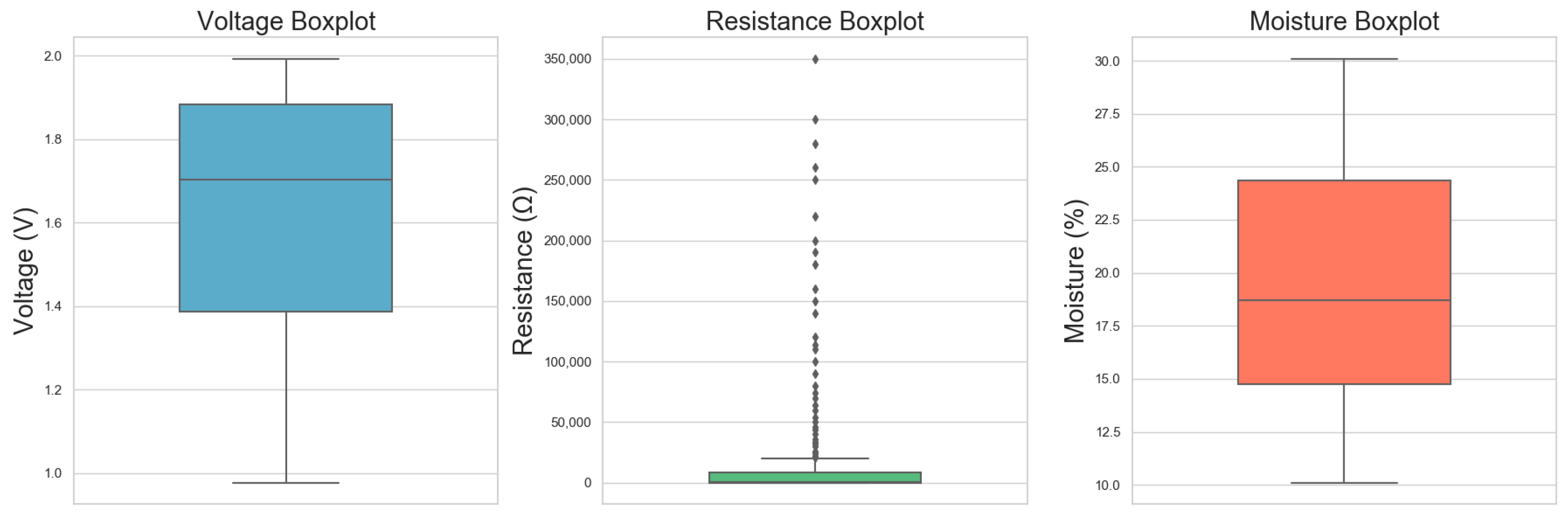
2.2. Data Preprocessing

Initially, data obtained from the grain moisture meter were cleaned. The initial dataset included voltage readings converted from the resistance of long-grain rice at 30 °C from over 100 different moisture groups and their corresponding moisture values. All incomplete records, i.e., those containing one or more missing values, were removed. The main reason for missing values is human recording errors that occurred during the recording process. In the processing, there were seven instances of data loss, which have been deleted. Removing incomplete records can improve the overall quality of the dataset. Since the training model dataset is relatively small, ensuring high-quality data input is crucial for establishing accurate and reliable models. Machine learning algorithms cannot directly handle missing values, so deleting records containing missing values provides a quick and simple solution, although it may not be the optimal one. Following this, outliers were identified and eliminated based on the boxplot [19] and the 3σ principle, as these may represent misreadings from the moisture meter or data entry errors. Some data also contain duplicate values, and the reason for the occurrence of these three duplicated data points is human errors during the recording process. Due to the voltage range in the homemade grain moisture meter being between 0 and 2.5 V, the small voltage span between moisture levels leads to the generation of duplicate values. Therefore, the samples are re-prepared to increase the voltage difference, aiming to minimize the occurrence of duplicate data points. Figure 1 displays a boxplot.
By utilizing box plots, a visually intuitive and concise statistical summary is provided for the data. The central line in the box plot represents the median of the data, which is the value located in the middle position after sorting all the data. The interquartile range can be used to assess the dispersion of the data, where a wider box indicates greater data dispersion. By placing multiple box plots side by side, it becomes convenient to compare the distribution of different datasets.
Subsequently, for handling missing values, the remaining missing values were also addressed by re-preparing the samples, conducting tests, and filling in the missing parts. Since the missing portions in this small dataset were not considerable, no multiple imputation methods [20] were employed. Following this, outlier treatment was performed by calculating the Z-score for each variable and removing outliers with Z-scores exceeding 3 in absolute value. The dataset comprises two feature columns, namely voltage values and resistance values, with a total of 125 data records, and the target feature for prediction is moisture content. In the above data processing steps, missing values and outliers are applied to both input features and target features. Finally, the Min–Max normalization method was applied to scale all feature values to the [0, 1] range to address issues related to different scales and magnitudes. A portion of the data are shown in Table 1, where the actual voltage values correspond to the voltage values used in the modeling set, while the measured voltage values are obtained from the self-made moisture meter.

3. System Modeling Method Construction

3.1. Support Vector Machine SVM Model Method

Support vector machines (SVMs) are a class of generalized linear classifiers that perform binary classification of data in a supervised learning manner. The decision boundary is the maximum-margin hyperplane solved from the learning samples, transforming the problem into one of solving a convex quadratic programming issue [21,22].
The performance of SVMs crucially depends on the choice of the kernel function method. The main kernel functions include linear, polynomial, Sigmoid, and Gaussian radial basis function (RBF) [23].
The kernel function calculation formula is as follows:
K X , Z = ( x ) ( z )
Formula (1) represents the calculation of the inner product directly in the feature space, and represents the process of mapping x to the inner product feature space.
(1) Linear Kernel.
K x i , x = x i T x
Formula (2) represents the inner product calculation in the original space of the data, functioning to align the data forms of the two spaces.
(2) Polynomial Kernel.
K x i , x = ( γ x i T x + r ) d
The polynomial kernel focuses on the global nature of the data. Direct calculation in polynomial space would lead to the curse of dimensionality, hence it includes a transformation process from high-dimensional space to low-dimensional space, where the inner product is calculated using the latter.
(3) Sigmoid Kernel.
K x i , x = t a n h ( γ x i T x + r )
The Sigmoid kernel approximates a multilayer perceptron neural network and focuses on the overall optimal value of the sample data.
(4) Gaussian radial basis kernel (RBF).
K x i , x = e x p ( γ | | x i x | | 2 )
Formula (5) transforms the original space into a feature space of infinite dimensions. Its effectiveness relies on the regulation of parameters γ , which possess significant adjustability, thereby making it extensively utilized in practical applications.
The importance of selecting a kernel function for the performance of SVMs is as follows:
(1) The kernel function defines the feature space: The kernel function determines how the data are mapped to a new feature space. Different kernel functions create different feature spaces.
(2) Curse of dimensionality: using a kernel function allows us to compute dot products in this high-dimensional space without explicitly mapping the data, thereby avoiding the computational and storage issues associated with the curse of dimensionality.
(3) Generalization ability of the model: a suitable kernel function can help the model learn more complex decision boundaries, thus leading to better generalization performance on unseen data.
(4) Complexity of the optimization problem: the choice of kernel function directly affects the complexity of the optimization problem in SVM.
(5) Data adaptability: different datasets may require different types of kernel functions.
Support Vector Regression (SVR) is a regression method based on the principles of support vector machines, used for predicting continuous numerical values. It incorporates most of the core concepts of SVMs, but unlike SVMs used for classification, the goal of SVR is to find a function that closely approximates all training samples within a predetermined tolerance range.
SVR attempts to learn a function, as shown in Formula (6):
f x = w · x + b
where ‘w’ is the weight vector and ‘b’ is the bias term. This function should be able to predict a result as close as possible to the true value ‘y’ for each input.
SVR has an important parameter, ‘ε’, known as the epsilon-insensitive loss, which means that when the absolute difference between the predicted value and the true value is within the range of ‘ε’, and it is not considered an error. This setting creates a tube (or boundary) centered around the prediction function with a width of ‘2ε’, where prediction errors within this interval are treated as zero.
The loss function is defined as in Formula (7):
L ε ( y , f ( x ) ) = m a x ( 0 , | y f ( x ) | ε )
To find the optimal ‘w’ and ‘b’, SVR solves the minimization problem:
1 2 | w | 2 + C i = 1 n δ i + δ i *
Subject to the constraint conditions as shown in Formula (9):
y i w · x i b ε + δ i w · x i + b y i ε + δ i *
where ‘ δ i ’ and ‘ δ i * ’ are slack variables, both greater than or equal to zero, used to handle data points that are not within the tube. ‘C’ is a regularization parameter that determines the model’s tolerance for errors.
SVR is a powerful regression tool that can handle linear and nonlinear relationships, and by selecting appropriate parameters, overfitting can be avoided. It is suitable for many practical regression tasks.

3.2. Sparrow Search Algorithm

The Sparrow Search Algorithm (SSA) is a relatively new swarm intelligence optimization algorithm, inspired by the foraging and predator evasion behaviors of sparrows. The SSA possesses commendable local search capabilities. During foraging, sparrows are divided into discoverers, who are responsible for providing the direction of foraging for the population, and joiners, who are responsible for following to obtain food. When sparrows perceive danger, they exhibit anti-predatory behavior, which updates the population’s position [24,25]. It is based on six hypothetical rules: 1. leaders and followers, 2. discoverers and sentinels, 3. safe areas and food sources, 4. sparrow vigilance behavior, 5. response to sudden events, and 6. flight behavior patterns, thereby simulating the social behavior and survival strategies of sparrows.
SSA uses these behavioral assumptions to simulate the social behavior and foraging strategy of sparrows, guiding the process of finding the global optimum. The algorithm updates the positions of the sparrows through iteration, eventually converging to the optimal or near-optimal solution.
Despite the advantages of the SSA over other optimization algorithms, the search for the optimal solution still relies on discoverers, which can easily get trapped in local optima. Additionally, followers and sentinels, although they make up the majority of the population, have weaker optimization abilities. Therefore, an improved method has been proposed [26].

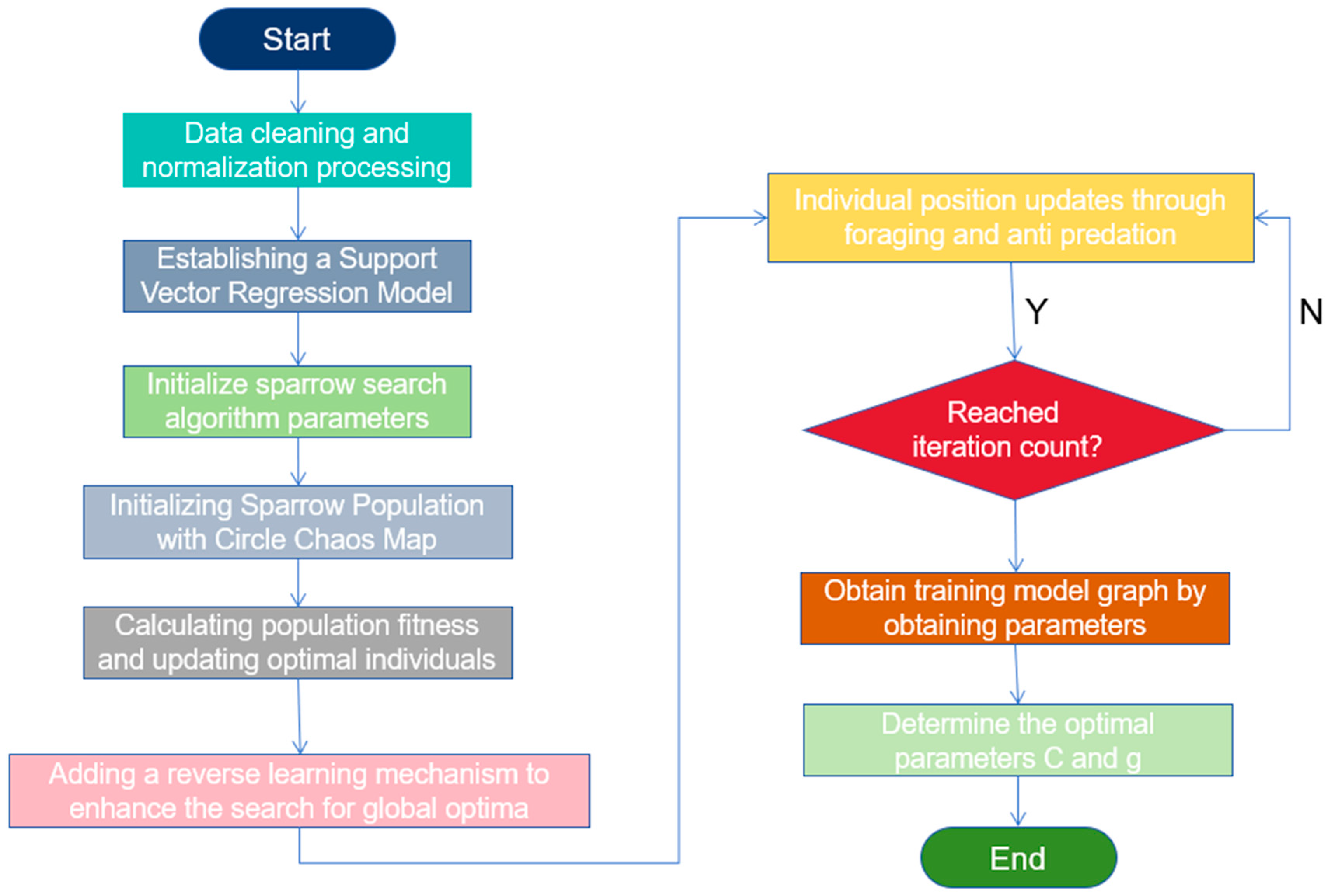
3.3. Improved Sparrow Search Algorithm

Building on the basis of the SSA algorithm, the Circle chaotic mapping is introduced first. Chaotic sequences exhibit good randomness and coverage, aiding the algorithm in exploring a broader solution space and avoiding premature convergence to local optima during the search process. By replacing the Sparrow Search Algorithm’s random initialization with chaos, population resources are more evenly distributed across the search space. The chaotic mapping helps rapidly approach the global optimal solution in the early stages of the search process and enhances convergence speed by effectively exploring different regions of the solution space. The formula is as follows:
x i + 1 = x i + 0.5 m o d ( 2.2 2 π s i n ( 2 π x i ) , i )
Since sentinels are often in poor positions, it is difficult for them to evade predators effectively. To address this issue, a reverse learning mechanism is introduced [27,28]. In the search process, if the algorithm gets trapped in a local optimum, the reverse learning mechanism can provide an effective escape strategy. By exploring the opposite position of the current solution, it may discover a better solution, allowing it to break out of the local optimum. Introducing reverse learning periodically helps maintain a balance between detailed local search and extensive global search, thus preventing premature convergence. When sentinels evade predators, they move in the opposite direction. With this improvement, sentinels can easily escape local optima, enhancing their ability to search for the global optimum.
The flowchart for constructing the improved SSA-SVR algorithm model is shown in Figure 2 [29,30].
Step one: This involves initializing the position and fitness of the sparrow population. This is carried out by assigning initial values to parameters N , n, PD, SD, and S T ;
Step two: begin the loop, iteration < N ;
Step three: sort the population to find the current optimal sparrow’s position and the best fitness;
Step four: start foraging behavior and update the discoverers’ positions according to Formula (7) [31,32].
X i , j t + 1 = X i , j t + 1 · e x p ( i a · N )     , i f   R 2 < S T X i , j t + 1 + Q · L                 , i f   R 2 S T
In the formula, N represents the maximum number of iterations. n represents the population size. PD represents the number of discoverers. SD represents the number of sparrows sensing danger. S T represents the safety value. R 2 represents the alert value, which is generated by a random number. Q represents a random number that follows a normal distribution. L represents a unit row vector. Lastly, ‘ a ’ represents a random number between 0 and 1.
Step five: update the joiners’ positions according to Formula (12).
X i , j t + 1 = Q · e x p ( X w o r s t X b e s t i 2 )                                 , i f   i > n / 2 X P t + 1 + X i , j X p t + 1 · A + · L     , o t h e r w i s e
In the formula, X w o r s t represents the position of the sparrow with the lowest fitness. A + is a row vector containing only elements 1 and −1 randomly.
Step six involves updating the position of the sparrow population to account for anti-predation behavior.
X i , j t + 1 = X b e s t t · β X i , j X b e s t t       , i f   f i > f b e s t X i , j t + K · ( X i , j X w o r s t f i f w o r s t + ε )     , i f   f i = f b e s t
In the formula, β is a random number that follows a normal distribution, and its function is to control the step size of the update position. K is the random number between [−1, 1], and f i is the individual fitness value. ε is a constant close to zero to avoid cases where the denominator is zero.
Formula (13) is the optimization of the normal sparrow search algorithm, determined by f i and f b e s t . In Formula (13), when f i is greater than f b e s t , the updated formula is difficult to use to complete the early warning task due to its own location limitations, so the reverse learning mechanism is added and the idea of reverse learning is introduced to replace Formula (14), as follows:
X i , j t = u b + l b r 3 · X i , j t     , f i > f b e s t
In the formula, u b and l b are the upper and lower limits of the current test function, respectively, and r 3 is a random number with the interval [0, 1].
Step seven: update the historical optimal fitness;
Step eight: End the loop when the maximum number of iterations is reached. Otherwise, perform steps three to seven.
The specific significance of using the improved SSA-SVR algorithm for establishing the grain moisture model is as follows:
(1) Automated parameter optimization.
Efficient parameter selection: the SSA can automatically find the optimal SVR parameters (such as penalty parameter C, insensitive loss ε, and RBF kernel γ parameter).
(2) Improved prediction accuracy.
Precise model fitting: with optimized parameters, the SVR model can fit the training data more accurately, thereby improving the prediction accuracy of grain moisture content while maintaining generalization ability.
(3) Enhanced model generalization ability.
Avoiding overfitting: the combination of SSA-optimized SVR by selecting appropriate parameter configurations not only accurately fits the training data but also avoids overfitting issues, ensuring that the model has good generalization ability on unknown data.
(4) Handling nonlinear problems.
Strong nonlinear fitting ability: SVR is particularly good at handling nonlinear relationships, which is often a typical nonlinear problem in predicting grain moisture content. Combined with SSA, the kernel function parameters of SVR can be effectively adjusted to enhance its modeling ability for complex nonlinear relationships.
(5) Strengthening the algorithm’s search capability.
Global search optimization: the SSA with Circle chaotic mapping and the reverse learning mechanism has stronger global search capability, helping to avoid local optima and potentially discovering SVR model parameters that are more suitable for the grain moisture model.
In conclusion, using the optimized SSA combined with SVR for training the grain moisture model enables automated parameter optimization, improves prediction accuracy and generalization ability, effectively handles nonlinear problems, adapts to the complexity of the data, and provides a powerful method for establishing grain moisture content models.

4. Results

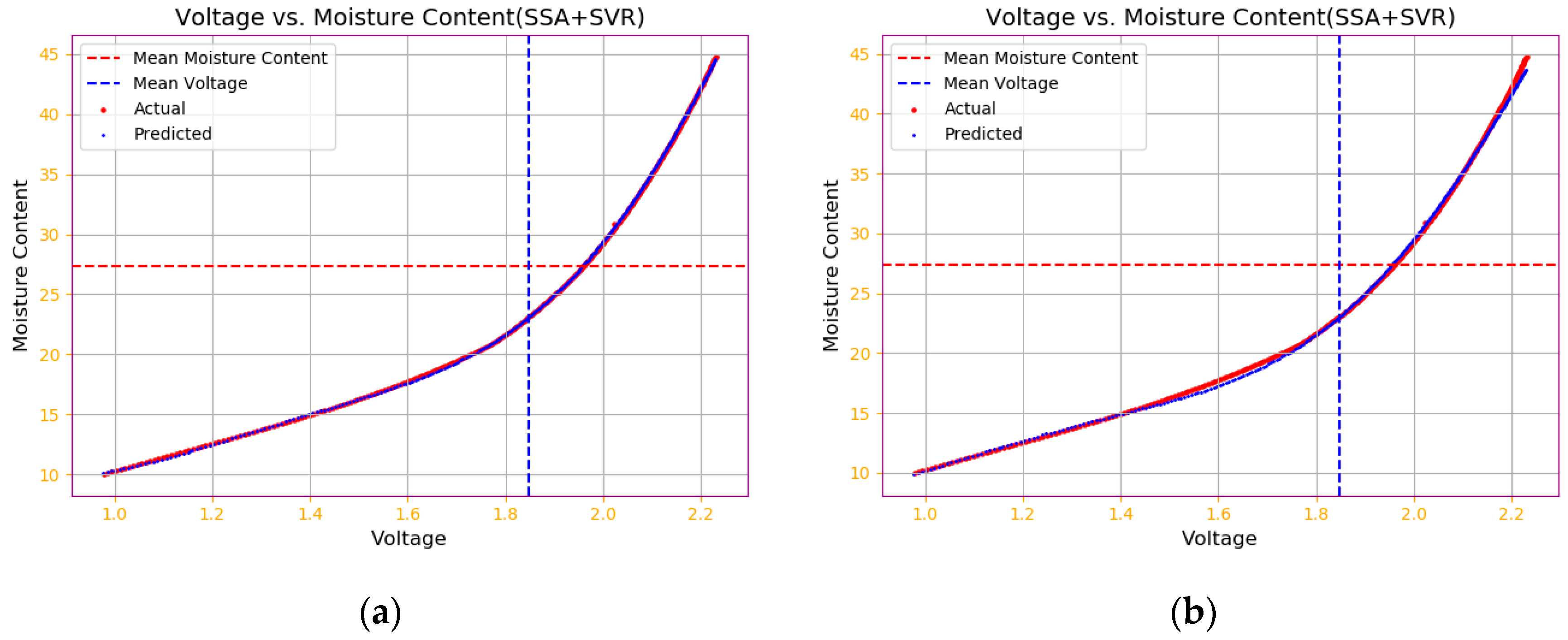
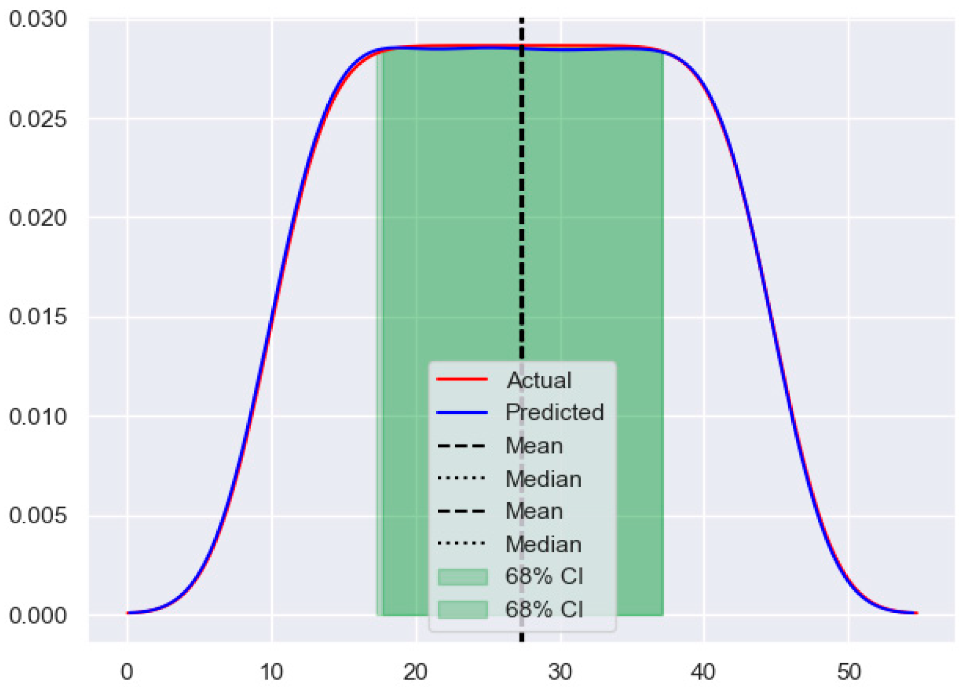
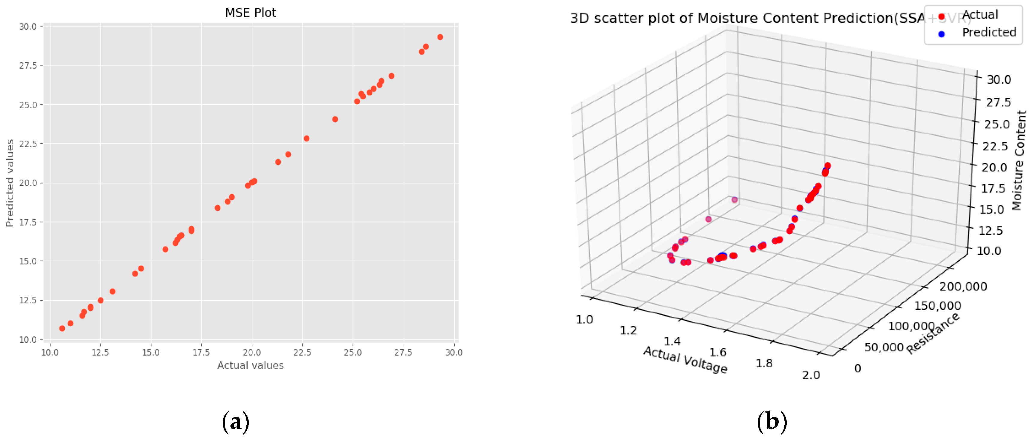
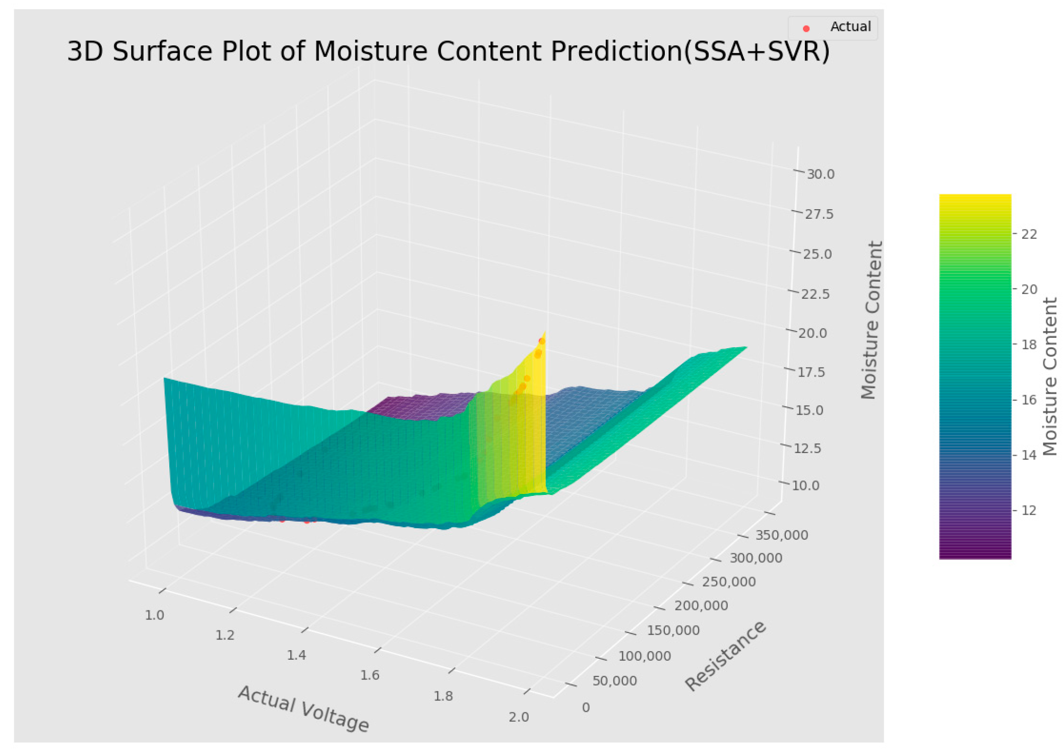
4.1. Improved SSA-SVR Training Model Results

To begin, choose the radial basis function with the kernel set to ‘rbf’ [33,34]. For parameter settings, utilize the GridSearchCV function to define the range of parameters. This includes the penalty parameter C, the width of the radial basis function gamma, and parameter ε for the epsilon-insensitive loss function.
First, initialize the SSA parameters. Since there is no ready-made Python library for the SSA, configure a detailed class to implement the details of the Sparrow Search Algorithm [35,36]. Set the initial population size to 45, the maximum number of iterations to 60, and include parameters for Circle chaotic mapping and the reverse learning mechanism. Apply reverse learning every 10 iterations, ensuring not to exceed the search space. The following is part of the SSA implementation configuration code:
The code “self.fitness[i] = self.obj_func(self.position[i])” is used to calculate fitness, the code “best_idx = np.argmin(self.fitness)” is used to find the best position, the code “self.update_producers(best_idx)” is the update producer location, the code “self.update_scouters(best_idx)” is the update alert location, the code “self.position = np.clip(self.position, self.lb, self.ub)” is to ensure that the search space is not exceeded, the code “best_idx = np.argmin(self.fitness), return self.position[best_idx], self.fitness[best_idx]” is to ensure that the search space is not exceeded, and the code “ssa = DetailedSSA(obj_func = objective_function, lb = −10, ub = 10, dim = 2, population_size = 45, max_iter = 60)” uses the SSA for optimization.
The fitness function formula is as follows:
F = m i n ( M S E T r a i n i n g S e t , T e s t i n g S e t )
In the formula, TrainingSet refers to the training set samples, and TestingSet refers to the test set samples. After using the sparrow search optimization algorithm, the fitness function becomes smaller, resulting in a decrease in the mean square error and an increase in the training accuracy of the model [37].
Set param_grid = {‘C’: [0.1, 1, 10], ‘epsilon’: [0.01, 1], ‘gamma’: [1, 10, 100]}, with 5-fold cross-validation [38,39], and the SSA will search for the optimal parameters within these ranges. Use the SSA parameters as described above; plot a two-dimensional scatter plot of voltage values and moisture values. When param_grid = {‘C’: [0.1, 1, 10, 100], ‘epsilon’: [0.01, 1], ‘gamma’: [0.001, 0.1, 1]}, add a random seed in the code, run the SSA-SVR model multiple times, meaning each run of the algorithm will start in a different initial state, generating different search paths and results. We calculate the average performance metrics of each run to obtain a general estimate of the model’s performance. By optimizing the SSA, the parameter combination obtained is the C penalty parameter as 72.3, the radial basis function width gamma as 0.75, and the epsilon insensitive loss as 0.2 [40], and with 5-fold cross-validation, the training model is relatively optimal, as shown in Figure 3a. Taking the average values, the correlation coefficient is 0.987, the coefficient of determination is 0.992, the root mean square error is 0.65, and the Best accuracy is 0.584. The “Best accuracy” reflects the highest average R2 score configuration obtained during the cross-validation process, where the dataset is divided into several small groups or “folds”. The model is trained using one fold as the test set and the rest as the training set in a rotating manner. This process is repeated multiple times, each time selecting a different fold as the test set. The average R2 score is based on the model’s performance on different subsets, providing a more robust estimate of the model’s generalization ability. Therefore, the actual Best accuracy is obtained through cross-validation, while the separately calculated R2 score is based on the model’s prediction of a specific dataset. Similarly, the closer the Best accuracy is to 1, the better the model parameter optimization, while close to 0 or negative values indicate poor training capabilities of the model. The training time is 0.49 s.
In Figure 3b, the training plot of the unimproved SSA-SVR model is shown. Taking the average values, the correlation coefficient is 0.947, the coefficient of determination is 0.938, the root mean square error is 1.92, and the Best accuracy is −0.89. The training time is 0.37 s. Compared to the improved SSA-SVR model, the unimproved model has significantly lower performance in all metrics except for the training time, which is relatively shorter.
Subsequently, the probability density map is added, as shown in Figure 4. The horizontal axis represents the value range of the data, and the vertical axis represents the probability density of the data points in the corresponding value range, so as to compare the distribution of the data set. This shows that the model training results are in high agreement with the real data.
In a homemade grain moisture meter, the voltage value obtained is determined by the resistance under a constant temperature. The corresponding moisture value is then found according to the corresponding national standard. Generally, within the moisture range of 9–20, there is a near-linear relationship between the grain’s internal moisture and the logarithm of its resistance. By taking data with moisture between 10 and 30, we can explore the relationship between resistance, voltage, and moisture values under the SSA + SVR model. Figure 5a shows the RMSE chart [41], Figure 5b displays the three-dimensional scatter plot, and Figure 6 depicts a three-dimensional surface plot.
The MSE plot in Figure 5a compares the actual values with the model training values. By plotting the scatter diagram of actual values against predicted values, the accuracy of the model predictions can be visually assessed. If the predicted values are very close to the actual values, the scatter points will tightly cluster around the 45-degree line (which represents the ideal one-to-one correspondence line). The MSE plot helps in visually evaluating the error distribution and prediction accuracy of the model. It can reveal patterns of prediction bias or the impact of outliers in the data on the model’s performance. Furthermore, as a performance metric, MSE quantifies the prediction errors of the model and provides guidance for optimizing model parameters and structure.
The combined use of the 3D surface plot in Figure 5b and Figure 6 provides rich information and a deep understanding of the model performance. In the scatter plot, each point represents an actual observation, where the position of the point indicates the values of voltage and resistance, while the color or size represents the actual moisture content. This allows observers to easily see the distribution of data points in three-dimensional space. The 3D surface plot illustrates the complex relationship between voltage, resistance, and moisture content. This three-dimensional visualization method can reveal the degree and patterns of influence of different input features (voltage and resistance here) on the target variable (moisture content). Through this plot, one can observe the trend of moisture content variation under different resistance and voltage conditions. By visualizing the impact of different features on the target variable, a method is provided for a deep understanding of the model behavior and data structure. This is valuable for evaluating the model’s complex nonlinear fitting ability and revealing the inherent relationships in the data. By comparing the actual data points in the 3D scatter plot with the predicted surface in the 3D surface plot, one can visually assess the model’s fit to the data. Ideally, the points should be closely distributed around the predicted surface, indicating that the model accurately captures the relationship between features and the target. In a three-dimensional space, it may be easier to identify anomalies that deviate from other data points or the predicted surface, which is very useful for further data cleaning and model optimization.
Print the moisture values obtained after model training in an Excel spreadsheet, where each voltage and resistance corresponds to a specific moisture value. Subsequently, using this table, one can directly look up the moisture value of long-grain rice by measuring the resistance of the long-grain rice at a temperature of 30 °C. This will enable a more timely and accurate assessment of the moisture content of the grains.
The above is based on a data model at 30 °C, and further explores the common relationship between temperature, voltage value, and moisture value in the range of 20 °C to 35 °C. Figure 7 is a three-dimensional surface chart of voltage, temperature, and moisture after the improved SSA-SVR algorithm.
Figure 7 shows a three-dimensional surface plot combining voltage, temperature, and moisture content based on the established optimal model. It first demonstrates the training results of different voltage values on moisture content, which are non-linear, highlighting the reason for using SVR for modeling. Another dimension reveals the influence of temperature on moisture content. By utilizing the improved SSA algorithm to find the optimal parameters, predictive performance on specific datasets can be enhanced, and a color gradient is used to represent the change in grain moisture with temperature and voltage. It can be observed that as the temperature increases and the voltage decreases, the moisture shows a significant change. The moisture values rise or fall by 0.1% for each 1 °C increase or decrease in temperature.

4.2. Other Model Training Results

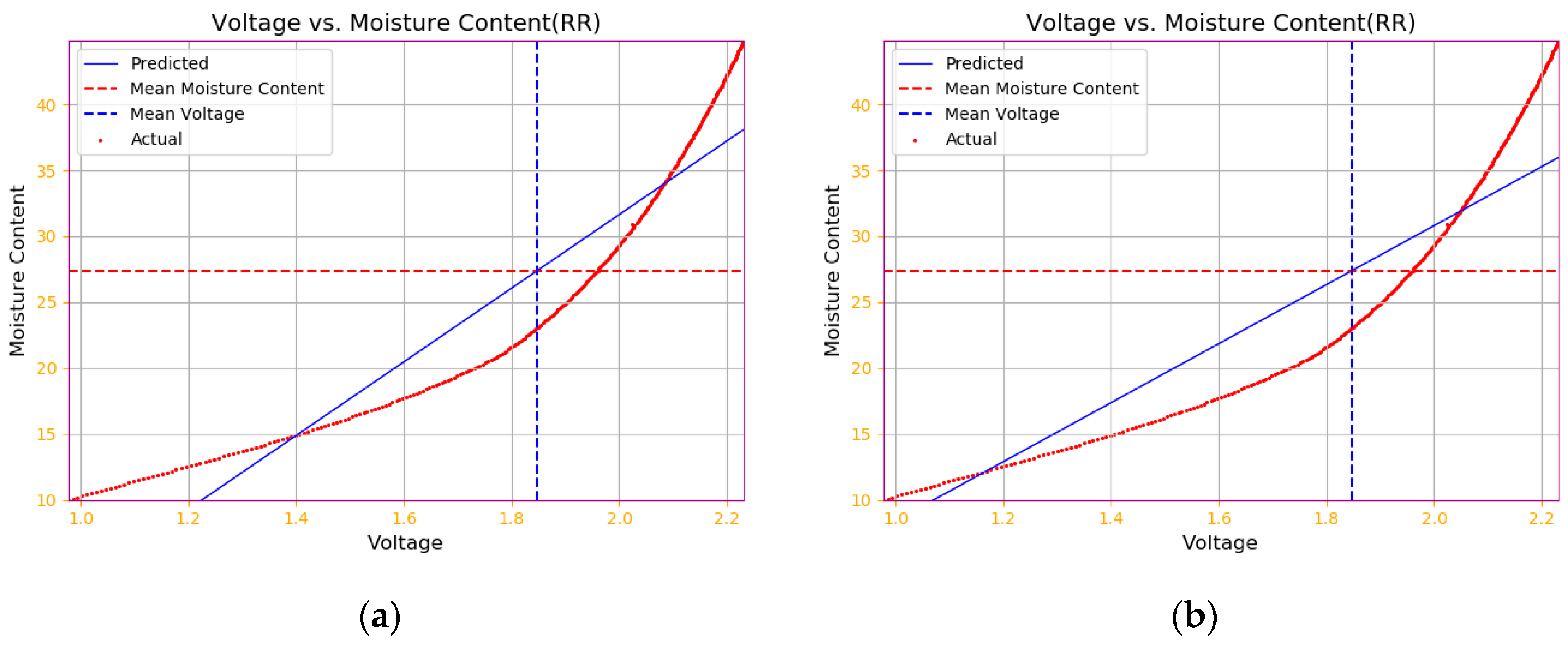
4.2.1. Ridge Regression Model Results

The ridge class from the scikit-learn library is implemented, where the alpha parameter specifies the strength of the regularization term. When the alpha parameter takes a small value, the regularization strength is weak, and the model tends to fit the training data more closely, leading to overfitting. Conversely, it may result in underfitting [42,43]. The fit() method is used to train the model. The default solver = ‘auto’ is used to automatically select a suitable solver for the data. Automatic selection means that in most cases ridge regression will select a suitable solver for the data, eliminating the need to specify it manually. By changing the value of the alpha parameter from 0.1 to 10, continuous model training is performed, as shown in Figure 8, where panel (a) is the training model with an alpha value of 0.1, and panel (b) is the training model with an alpha of 10.
When adjusting the alpha parameter, the correlation coefficient is 0.92, the determination coefficient is 0.86, and the root mean square error is 3.84 at an alpha value of 0.1. Similarly, at an alpha value of 10, the correlation coefficient is 0.92, the determination coefficient is 0.83, and the root mean square error is 4.20. Figure 8a,b, as well as the correlation coefficient, indicate that ridge regression is not very suitable for predicting this dataset due to a significant deviation.
The reasons for choosing ridge regression as a comparative algorithm to build the model are as follows:
(1) Handling multicollinearity: ridge regression addresses the issue of collinearity among features by adding an L2 regularization term to the loss function, which helps in dealing with highly correlated datasets.
(2) Preventing overfitting: the regularization term penalizes the complexity of the model, aiding in reducing overfitting on the training data and improving the model’s generalization ability.
(3) Baseline for linear models: as a linear model, ridge regression is often used as a baseline for comparison to assess whether nonlinear models can significantly outperform it on the same problem.

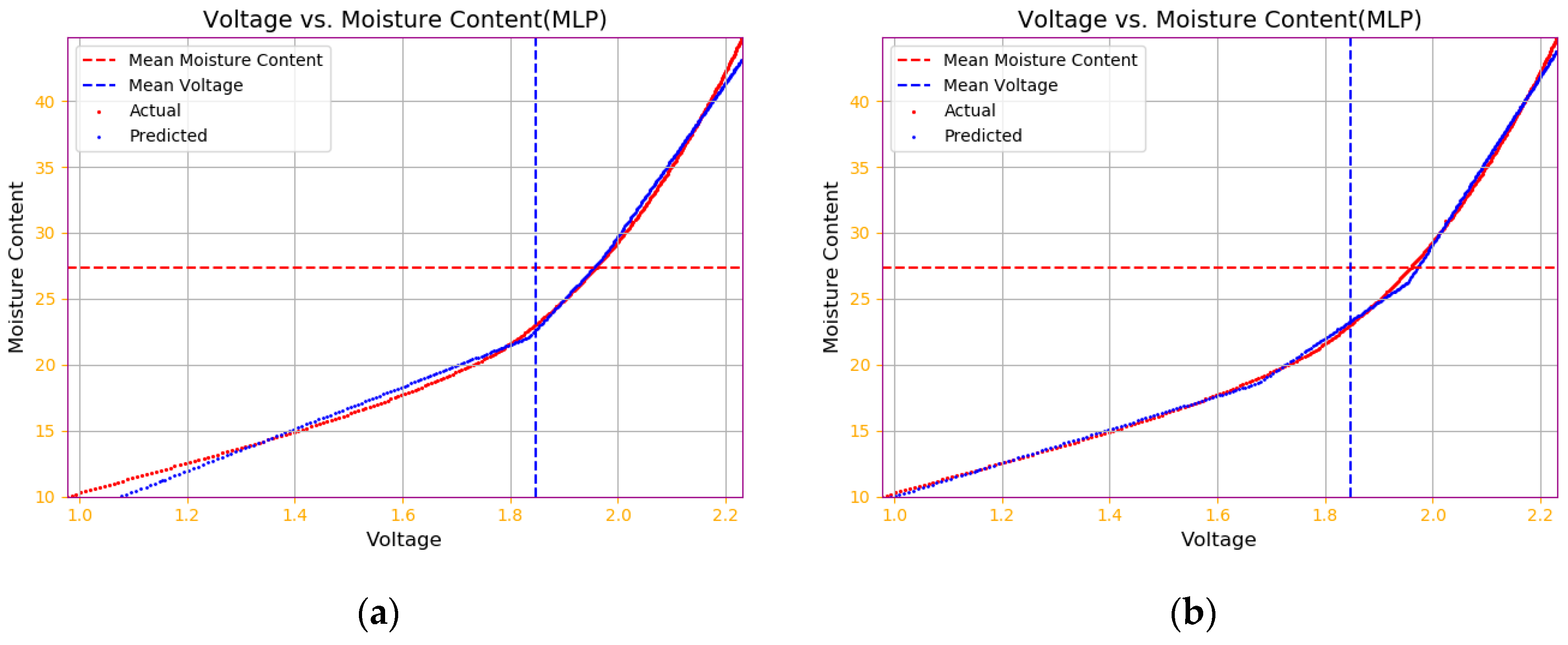
4.2.2. MLP Model Results

To establish a Multi-Layer Perceptron (MLP) model using the MLP regressor from scikit-learn, first create an instance of the MLP regressor with two hidden layers specified. We set the hidden_layer_sizes = (7, 3), indicating that the model has two hidden layers—the first layer contains seven neurons, and the second layer contains three neurons. The model is trained using the Adam optimizer, which is an adaptive learning rate stochastic optimization algorithm known for achieving good performance. Due to the small-scale dataset in this paper, one to two hidden layer structures are sufficient to avoid overfitting [44,45]. The activation function is initially set to the Relu function:
f x = m a x ( 0 , x )
The Rectified Linear Unit (ReLU) function outputs the positive part of the input, which is max(0, x). Its purpose is to set all negative input values to 0 while leaving positive input values unchanged. It is a simple non-linear transformation that provides non-linearity in practice, avoids the vanishing gradient problem, and is computationally efficient. The characteristic of the ReLU function maintaining active gradients in the positive range helps alleviate the vanishing gradient problem during training and can improve runtime speed.
This model has a large deviation, and the curve is not stable. In subsequent identical training sessions, significant differences in the model graphs are observed. When modifying parameters by changing hidden_layer_sizes from (7, 3) to (10, 5) and using the tanh function as the activation function, the following is achieved:
f x = e x e x e x + e x
By changing the maximum number of iterations to 10,000, we obtained a relatively optimal model. This model has a correlation coefficient of 0.96, a determination coefficient of 0.95, and a root mean square error of 2.69. The training time for this model was 4.02 s. The training model is shown in Figure 9b.
The reasons for selecting MLP as a comparative algorithm to establish a model are as follows:
(1) Strong nonlinear modeling capability: MLP is a fundamental deep learning model capable of capturing complex nonlinear relationships in data, making it suitable for handling problems that are nonlinearly separable.
(2) High flexibility: by adjusting the number of network layers and neurons in each layer, MLP can be designed to adapt to various tasks of different complexities.

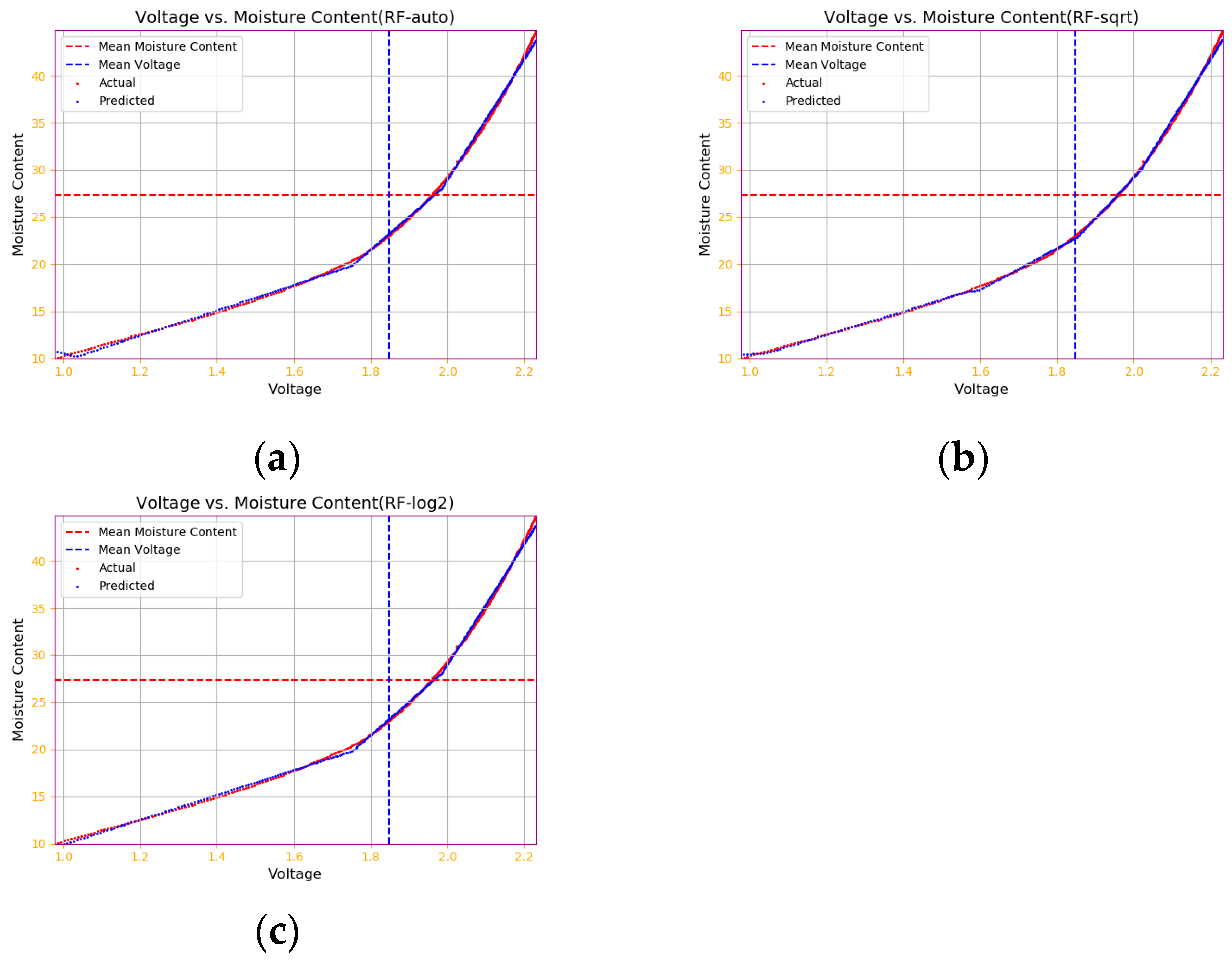
4.2.3. Random Forest Model Results

To make the output model more accurate in the use of random forest models, grid search has been added. Although this increases the code execution time and affects efficiency, grid search can try different parameter combinations to find the best model parameters. It also avoids the tedious process and subjectivity of manually adjusting parameters.
The parameter grid param_grid contains some important parameters of the random forest model and their corresponding value ranges. A search is conducted within this grid to find the optimal parameter combination for building the random forest model. The random forest model utilizes the RandomForestRegressor from scikit-learn. The initial code for this section is as follows:
param_grid = {
 ‘n_estimators’: [50, 100, 200, 300],
 ‘max_depth’: [None],
 ‘min_samples_split’: [2, 5, 10],
 ‘min_samples_leaf’: [1, 2, 4]
}
‘n_estimators’ refers to the number of decision trees. ‘max_depth’ refers to the maximum depth of the decision trees, where None means there is no limit to the depth of the trees. ‘min_samples_split’ refers to the minimum number of samples required to split an internal node. ‘min_samples_leaf’ refers to the minimum number of samples required at a leaf node [46,47]. In training, these parameters are exhaustively searched in combination to construct the random forest model and estimate its performance. Ultimately, the optimal model parameters are selected as the best performing parameter combination.
Iterate through different max_features options (which impact the number of features considered for each split in the tree) to evaluate model performance, using cross-validation (cross_val_score) to obtain average scores. Select the best performing max_features value and retrain the model. Setting max_features = ‘auto’ means considering all features at each split. To ensure the reliability of the results, use different random seed values to help evaluate the model [48]. Train several different models and compare how different max_features values affect model performance.
Figure 10a–c correspond to the cases where max_features are ‘auto’, ‘sqrt’, and ‘log2’, respectively. In the model trained with max_features = ‘auto’, although the correlation coefficient and determination coefficient both reached 0.96 and the root mean square error was 1.98, the Best accuracy was between −7 and −9, which is relatively poorer compared to that of the improved SSA-SVR.
The reasons for selecting random forest as a comparative algorithm to establish the model are as follows:
(1) Resistance to overfitting ensemble method: Random forest builds multiple decision trees and makes final decisions through voting. This ensemble learning method effectively resists overfitting, enhancing the stability and accuracy of the model.
(2) Feature selection: random forest evaluates the importance of features during training, providing insights into understanding how the model makes predictions and which features are more important.
(3) Strong adaptability: random forest can handle high-dimensional data without the need for feature scaling, making it suitable for various types of data, including classification and regression problems.

4.3. Comparison of Algorithm Model Performance

Table 2 compares the performance of the improved SSA + SVR model with the default settings of three other algorithms at the beginning.

5. Conclusions

Based on a self-made resistance-type grain moisture meter, this study involved placing long-grain rice into the moisture meter at a room temperature of 30 °C to obtain resistance values, voltage values, and corresponding moisture values. The voltage value obtained was considered the actual voltage value and used as the prediction set. Subsequently, the same batch of samples was placed into a PM-2500 model single-grain automatic moisture meter produced by the Japanese company Kett to obtain the moisture values of the grains. Based on these moisture values, the corresponding voltage value in the fitting curve of the homemade moisture meter was determined and considered the true voltage value and used as the modeling set. The improved SSA-SVR method was employed to train the grain moisture model. This algorithm combination can better handle time series data, extract useful features, and accurately predict grain moisture. Through model training, the grain moisture value can be quickly obtained directly from measuring the resistance value under certain temperature conditions, reducing the interference of environmental factors such as humidity and temperature on measurement results. This research may potentially improve the speed and accuracy of moisture measurement during on-site drying processes, as the model directly correlates resistance values to moisture values, reducing the influence of environmental factors compared to traditional moisture detection methods. If the model demonstrates stability under different environments and conditions, it will prove its strong applicability and broad potential for promotion [49]. Additionally, comparisons were made between models established using ridge regression, multilayer perceptron, random forest methods [50,51], and the improved SSA-SVR method, showing that the latter exhibited superior performance in terms of correlation coefficient, determination coefficient, and RMSE.
During the modeling process, the first challenge lies in the limitations of data quality and quantity. Initially, the sample preparation faced difficulties due to unfamiliar operational procedures, resulting in some waste and insufficient sample quantity. Subsequently, the same brand of long-grain rice was repurchased for sample preparation. Additionally, during the data collection process, there were some outliers that required preprocessing. While these issues are controllable, the moisture content of grains can fluctuate due to environmental conditions and storage methods, leading to inaccurate data, which is a drawback of this study. The second challenge pertains to the selection of parameters in the algorithm, such as the type of kernel function and regularization parameters. It is essential to find relatively suitable parameters for simulation training and choose the optimal parameters to prevent model overfitting or underfitting. The third limitation arises from the increased computational cost after introducing chaotic mapping and reverse learning mechanisms, requiring more iterations for convergence and extended training time. However, since the dataset is not large-scale, the impact of this aspect is relatively minor. Lastly, Support Vector Regression (SVR) is a black-box model with an opaque decision-making process, potentially limiting model interpretability and user trust. Moreover, SSA is used to extract the main components of time series data, but explaining the relationship between these components and grain moisture content is challenging, representing the major drawback of this study. This research merely establishes a model to quickly obtain the moisture content of long-grain rice in drying sites, providing a relatively new approach to grain moisture detection.
This article has the following potential impacts on the grain industry:
(1) Improve quality control during storage and transportation of grains: accurate moisture measurement is crucial for controlling grain quality, preventing mold growth, and extending shelf life.
(2) Optimize the drying process: it can help grain warehouse managers or farmers to dry grains more quickly and effectively, saving energy and reducing the risks of over-drying or under-drying.
(3) Increase grain processing efficiency: The moisture content of grains affects processing quality and costs. A faster and more accurate detection method can optimize the processing flow and improve the quality of the final products.
(4) Promote industry automation: it helps simplify the moisture measurement process, providing automation for the grain industry, thereby reducing labor costs and improving efficiency.
In future work, in terms of parameter optimization, it may be beneficial to explore a broader or more detailed parameter space and experiment with different search strategies (such as random search or Bayesian optimization) to potentially find more optimal parameter combinations. In model selection, trying out different kernel functions could be considered to see if there are better choices for the current dataset. For data processing, using data augmentation techniques (such as adding noise to data or utilizing data generation techniques) to increase the diversity of training data can help improve the model’s generalization ability. In evaluation methods, considering other performance metrics (such as model computational efficiency, memory usage, etc.) as optimization objectives could strike a balance between performance and efficiency.

Author Contributions

Conceptualization, W.C. and G.L.; methodology, G.L.; software, G.L. and B.Q.; validation, H.S., B.Q. and Z.L.; investigation, Z.L.; resources, H.S.; writing—original draft preparation, G.L.; writing—review and editing, W.C.; supervision, W.C. All authors have read and agreed to the published version of the manuscript.

Funding

This work is supported by the Education Department of Jilin Province for its financial support through grant number JJKH20220757CY, and the Jilin Province Science and Technology Development Project for the grant number 20220204138YY.

Data Availability Statement

The data presented in this study are available in article.

Conflicts of Interest

The authors declare no conflicts of interest.

References

  1. Lin, G. Research on Online Detection and Control System for Grain Moisture Content; Shenyang University of Technology: Shenyang, China, 2003. [Google Scholar]
  2. Sun, J.; Zhou, Z.; Tang, H. Research on Rapid Detection Methods for Grain Moisture at Home and Abroad. Grain Storage 2017, 3, 46–49. [Google Scholar]
  3. Liu, Z. Research on Online Monitoring Instrument for Grain Moisture; Jilin Agricultural University: Changchun, China, 2013. [Google Scholar]
  4. Sun, Y. Research on Capacitive Grain Moisture Online Detection Instrument; Jilin Agricultural University: Changchun, China, 2014. [Google Scholar]
  5. Shi, Y. Design and Implementation of a Grain Moisture Measuring Instrument; Jilin University: Changchun, China, 2018. [Google Scholar]
  6. Ding, Y.; Zhang, X.; Wang, X. Overview of Grain Moisture Measurement Technology. Anal. Instrum. 2005, 2, 5–8. [Google Scholar]
  7. Xue, J.; Shen, B. A novel swarm intelligence optimization approach: Sparrow search algorithm. Syst. Sci. Control Eng. 2020, 8, 22–34. [Google Scholar] [CrossRef]
  8. Lyu, X.; Mu, X.; Zhang, J.; Wang, Z. Chaotic sparrow search optimization algorithm. J. Beijing Univ. Aeronaut. Astronaut. 2021, 47, 1712–1720. [Google Scholar]
  9. Mao, Q.; Zhang, Q. Improved sparrow algorithm combining cauchy mutation and opposition-based learning. J. Front. Comput. Sci. Technol. 2021, 15, 1155–1164. [Google Scholar]
  10. Tang, Y.; Li, C.; Song, Y.; Chen, C.; Cao, B. Adaptive mutation sparrow search optimization algorithm. J. Beijing Univ. Aeronaut. Astronaut. 2023, 49, 681–692. [Google Scholar]
  11. Zhang, W.; Liu, S.; Ren, C. Mixed strategy improved sparrow search algorithm. Comput. Eng. Appl. 2021, 57, 74–82. [Google Scholar]
  12. Boateng, E.Y.; Otoo, J.; Abaye, D.A. Basic tenets of classification algorithms K-nearest-neighbor, support vector machine, random forest and neural network: A review. J. Data Anal. Inf. Process. 2020, 8, 341–357. [Google Scholar] [CrossRef]
  13. Chai, T.; Draxler, R.R. Root mean square error (RMSE) or mean absolute error (MAE). Geosci. Model Dev. Discuss. 2014, 7, 1525–1534. [Google Scholar]
  14. Xiang, W. Standardization of Moisture Content in Food and Its Determination Methods. Chin. Foreign Med. 2009, 28, 174–175. [Google Scholar]
  15. Su, Y. Discussion on the calibration method of the drying method moisture analyzer. Shanghai Metrol. Test. 2009, 4, 9–11. [Google Scholar]
  16. Hu, J.; Li, Z.; Pan, X. Dispersive Field Capacitive Grain Moisture Sensor and Its Application in Grain Storage. Chin. J. Cereals Oils 2017, 32, 108–111. [Google Scholar]
  17. Nelson, S.O.; Russell, R.B. Models for Estimating the Dielectric Constants of Cereal Grains and Soybeans. J. Microw. Power Electromagn. Energy 1986, 21, 110–113. [Google Scholar]
  18. Kraszewski, A.; Nelson, S.O. Composite model of the complex permittivity of cereal grain. J. Agric. Eng. Res. 1989, 43, 211–219. [Google Scholar] [CrossRef]
  19. Yoav, B. Opening the Box of aBoxplot. Am. Stat. 1988, 42, 257–262. [Google Scholar]
  20. Pang, X. Algorithm Implementation of Multiple Interpolation Processing Method for Missing Data. Stat. Decis.-Mak. 2012, 24, 18–22. [Google Scholar]
  21. Lin, C.; Wang, S. Fuzzy Support Vector Machines. IEEE Trans. Neural Netw. 2002, 3, 464–471. [Google Scholar]
  22. Cortes, C.; Vapnik, V. Support-vector Networks. Mach. Learn. 1995, 20, 273–297. [Google Scholar] [CrossRef]
  23. Tyagi, D.; Verma, A.; Sharma, S. An improved method for face recognition using local ternary pattern with GA and SVM classifier. In Proceedings of the 2016 2nd International Conference on Contemporary Computing and Informatics (IC3I), Noida, India, 14–17 December 2016; pp. 421–426. [Google Scholar]
  24. Li, D.A. Hybrid Sparrow Search Algorithm. Comput. Knowl. Technol. 2021, 17, 232–234. [Google Scholar]
  25. He, H.; Ma, X.; Wang, H.; Fan, S.; Han, L. Multi-threshold Segmentation of Forest Fire Image Based on Improved Sparrow Search Algorithm. Sci. Technol. Eng. 2021, 21, 11263–11270. [Google Scholar]
  26. Mao, Q.; Zhang, Q.; Mao, C.; Bai, J.X. Mixing Sine and Cosine Algorithm With Levy Flying Chaotic Sparrow Algorithm. J. Shanxi Univ. (Nat. Sci. Ed.) 2021, 44, 1086–1091. [Google Scholar]
  27. Zhang, Z.; He, R.; Yang, K. A Bioinspired Path Planning Approach for Mobile Robots Based On Improved Sparrow Search Algorithm. Adv. Manuf. 2022, 10, 114–130. [Google Scholar] [CrossRef]
  28. Zhang, L.; Wang, T.; Zhou, H. A Multi Strategy Improved Sparrow Search Algorithm. Comput. Eng. Appl. 2022, 58, 133–140. [Google Scholar]
  29. Ye, Y.B.; Li, R.C.; Xie, M.; Wang, Z.; Ba, Q. A state evaluation method for a relay protection device based on SSA–SVM. Power Syst. Prot. Control. 2022, 50, 171–178. [Google Scholar]
  30. Najafzadeh, M.; Niazmardi, S. A Novel Multiple-Kernel Support Vector Regression Algorithm for Estimation of Water Quality Parameters. Nat. Resour. Res. 2021, 30, 3761–3775. [Google Scholar] [CrossRef]
  31. Lan, Z.; He, Q. Multi-trategy Fusion Algorithm and Its Engineering Optimization. Appl. Res. Comput. 2022, 39, 758–763. [Google Scholar]
  32. Xu, X.; Peng, L.; Ji, Z. Research on Substation Project Cost Prediction Based on Sparrow Search Algorithm Optimized BP Neural Network. Sustainability 2021, 13, 13746. [Google Scholar] [CrossRef]
  33. Ren, J.; Cui, J.; Dong, W.; Xiao, Y.; Xu, M.; Liu, S.; Wan, J.; Li, Z.; Zhang, J. Remote Sensing Inversion of Typical Offshore Water Quality Parameter Concentration Based on Improved SVR Algorithm. Remote Sens. 2023, 15, 2104. [Google Scholar] [CrossRef]
  34. Zhang, J.; Zhang, Y.; Chen, L.; Wang, Q.; Zhao, M. Water Quality Prediction for Hanjiang with Optimized Support Vector Regression. In Proceedings of the 2019 IEEE 8th Data Driven Control and Learning Systems Conference (DDCLS), Dali, China, 24–27 May 2019; pp. 832–837. [Google Scholar]
  35. Sulandari, W.; Subanar, S.; Suhartono, S.; Utami, H.; Lee, M.H.; Rodrigues, P.C. SSA-Based Hybrid Forecasting Models and Applications. Bull. Electr. Eng. Inform. 2020, 9, 2178–2188. [Google Scholar] [CrossRef]
  36. Tabatabaei, S.M.; Attari, N.; Panahi, S.A.; Asadian-Pakfar, M.; Sedaee, B. EOR Screening Using Optimized Artificial Neural Network by Sparrow Search Algorithm. Geoenergy Sci. Eng. 2023, 229, 212023. [Google Scholar] [CrossRef]
  37. Xu, X.; Wang, J.; Wu, J.; Qu, Q.; Ran, Y.; Tan, Z.; Luo, M. Full-Waveform LiDAR Echo Decomposition Method Based on Deep Learning and Sparrow Search Algorithm. Infrared Phys. Technol. 2023, 130, 104613. [Google Scholar] [CrossRef]
  38. Basak, D.; Pal, S.; Patranabis, D.C. Support Vector Regression. Process. Lett. Rev 2007, 11, 203. [Google Scholar]
  39. Zhang, F.; O’Donnell, L.J. Support Vector Regression. In Machine Learning; Academic Press: New York, NY, USA, 2020; pp. 123–140. [Google Scholar]
  40. Duan, S.; Liu, S. Research on Temperature Compensation of Fiber Optic Pressure Sensor Based on SSA-SVR. Electron. Devices 2023, 46, 1268–1274. [Google Scholar]
  41. Hodson, T.O. Root-mean-square error (RMSE) or mean absolute error (MAE): When to use them or not. Geosci. Model Dev. 2022, 15, 5481–5487. [Google Scholar] [CrossRef]
  42. Hoerl, A.E.; Kennard, R.W. Ridge regression: Biased estimation for nonorthogonal problems. Technometrics 1970, 12, 55–67. [Google Scholar] [CrossRef]
  43. Boonstra, P.S.; Mukherjee, B.; Taylor, J.M. A small-sample choice of the tuning parameter in ridge regression. Stat. Sin. 2015, 23, 1185. [Google Scholar] [CrossRef]
  44. Wu, Y.; Wang, S. A New Fast Convergent Backpropagation Algorithm. J. Tongji Univ. (Nat. Sci. Ed.). 2004, 32, 1092–1095. [Google Scholar]
  45. Zhang, G.; Yin, J.; Zhu, E. A New method of calculating the upper limit on multilayer perceptron’s hidden neuron number. Comput. Eng. Sci. 2007, 29, 137–139. [Google Scholar]
  46. Breiman, L. Random forests. Mach. Learn. 2001, 45, 5–32. [Google Scholar] [CrossRef]
  47. Wang, F.; Wang, Y.; Zhang, K.; Hu, M.; Weng, Q.; Zhang, H. Spatial heterogeneity modeling of water quality based on random forest regression and model interpretation. Environ. Res. 2021, 202, 111660. [Google Scholar] [CrossRef]
  48. Xing, S.; Gao, G.; Zhang, Z. Short-term load forecasting model based on double-layer random forest algorithm. Guangdong Electr. Power 2019, 32, 160–166. [Google Scholar]
  49. Ülker, E.D.; Ülker, S. Modelling the currency exchange ratesusing support vector regression. In Intelligent Computing: Proceedings of the 2020 Computing Conference; Springer: London, UK, 2020; pp. 326–333. [Google Scholar]
  50. Zhang, R.; Wang, Y. Research on Machine Learning and Its Algorithms and Development. Commun. Univ. China Newsp. (Nat. Sci. Ed.) 2016, 23, 10–18+24. [Google Scholar]
  51. Meena, L.; Chaurasiya, V.K.; Purohit, N.; Singh, D. Comparison of SVM and random forest methods for online signature verification. In Proceedings of the 12th International Conference on Intelligent Human Computer Interaction, Daegu, Republic of Korea, 24–26 November 2020; Springer: Berlin/Heidelberg, Germany, 2021; pp. 288–299. [Google Scholar]
Figure 1. Data cleaning box diagram.
Applsci 14 03171 g001
Figure 2. Improved SSA-SVR algorithm flowchart.
Applsci 14 03171 g002
Figure 3. (a) Shows the improved SSA-SVR training model diagram; (b) shows the train model diagram for SSA-SVR.
Applsci 14 03171 g003
Figure 4. Improved SSA-SVR probability density diagram.
Applsci 14 03171 g004
Figure 5. (a) Shows the RMSE diagram; (b) way to improve the SSA + SVR 3D scatter plot.
Applsci 14 03171 g005
Figure 6. Improved SSA + SVR 3D surface map.
Applsci 14 03171 g006
Figure 7. Three-dimensional surface diagram of voltage, temperature, and moisture.
Applsci 14 03171 g007
Figure 8. (a) Shows the training graph of the alpha = 0.1 model; (b) training graph for alpha = 10 model.
Applsci 14 03171 g008
Figure 9. (a) Shows MLP model training; (b) training the optimized MLP model.
Applsci 14 03171 g009
Figure 10. (a) Shows the training model with max_features = ‘auto’; (b) shows the training model with max_features = ‘sqrt’; and (c) shows the training model with max_features = ‘log2’.
Applsci 14 03171 g010
Table 1. Results of data processing section.
Partial Data Related to Long-Grain Rice at 30 °C
Resistance Value (K)True Voltage Value (V)Actual Voltage Value (V)Measured Moisture Value (%)
26,0001.24761.248113.3
80001.38191.381214.6
12001.61451.615318.1
4601.73021.729119.6
1101.86991.870524.1
611.92201.922125.6
162.01872.019430.1
Table 2. Performance comparison of various models.
Correlation CoefficientCoefficient of DeterminationRMSETraining Time
SSA-SVR0.940.931.420.32
(Improvement) SSA-SVR0.990.980.850.49
RR0.920.863.840.57
MLP0.940.932.993.84
RF0.950.961.830.85
Disclaimer/Publisher’s Note: The statements, opinions and data contained in all publications are solely those of the individual author(s) and contributor(s) and not of MDPI and/or the editor(s). MDPI and/or the editor(s) disclaim responsibility for any injury to people or property resulting from any ideas, methods, instructions or products referred to in the content.

