Abstract
Physics-Informed Neural Network (PINN) is a data-driven solver for partial and ordinary differential equations (ODEs/PDEs). It provides a unified framework to address both forward and inverse problems. However, the complexity of the objective function often leads to training failures. This issue is particularly prominent when solving high-frequency and multi-scale problems. We proposed using transfer learning to boost the robustness and convergence of training PINN, starting training from low-frequency problems and gradually approaching high-frequency problems through fine-tuning. Through two case studies, we discovered that transfer learning can effectively train PINNs to approximate solutions from low-frequency problems to high-frequency problems without increasing network parameters. Furthermore, it requires fewer data points and less training time. We compare the PINN results using direct differences and relative error showing the advantage of using transfer learning techniques. We describe our training strategy in detail, including optimizer selection, and suggest guidelines for using transfer learning to train neural networks to solve more complex problems.
1. Introduction
Physics-Informed Neural Networks (PINNs) are a relatively new data-driven solver of partial differential equations (PDEs) [1,2,3]. The neural networks’ capability to approximate complex functions is their basis for solving partial differential equations. While the idea of using neural networks to estimate PDE solutions dates back to the 1990s, it initially garnered limited attention for various reasons. With the rapid advancements in deep neural network technology, the exponential growth in computing power, and the thriving open deep learning community, PINNs have recently garnered substantial interest and acclaim.
PINNs possess several notable advantages that make them a competitive method compared to mature, traditional numerical approaches for PDEs. PINN, as a meshless method, directly embeds mathematical equations into the network structure. The dual reliance on observational data and mathematical models equips PINNs to handle noisy observational data. Moreover, a PINN offers a consistent framework for forward and inverse problems through optimization algorithms [3]. By simply extending the neural network with additional output channels, PINNs can be employed to solve inverse problems. In inverse design, PINNs can impose PDEs as rigorous constraints, enhancing their utility. While neural networks grapple with the curse of dimensionality as problems become more complex, PINNs strive to resolve PDEs and their inversion challenges in domains characterized by intricate geometries and high dimensions, where numerical simulations are notably challenging. PINNs have produced compelling results on various problems in computational science and engineering, such as computational fluid dynamics [4], acoustics [5], solid mechanics [6], elastodynamics [7,8,9], and geo-physics [10,11,12].
However, training PINNs to achieve fast convergence and accuracy is a persistent challenge. This challenge is intricately linked to the highly complex and non-convexity of the loss function, which makes a PINN hard to train [13,14]. Furthermore, training PINNs also suffers from spectral bias. The neural networks prioritize learning low-frequency patterns over high-frequency details [15,16]. When the problem contains high-frequency features, the PINN models often fail to converge to the desired solution due to this phenomenon [17,18,19]. PINNs’ inherent ability to encapsulate domain knowledge and exploit neural network architectures has made them particularly attractive for simulating complex physical systems. However, as the applications of PINNs extend to problems characterized by high-frequency oscillations and intricate multi-scale phenomena, they face significant hurdles. These challenges often manifest in numerical instability, slow convergence, and increased computational demands, making it imperative to develop strategies that enhance the robustness and efficiency of PINNs in such scenarios.
The primary objective of this research is to elucidate the prevailing challenges encountered in PINNs when applied to high-frequency and multi-scale problems. To mitigate these challenges, we investigate the utility of transfer learning. By incorporating transfer learning into the PINN framework, we aim to harness the benefits of pre-trained models and transferable knowledge, potentially enhancing the convergence and accuracy of PINNs for high-frequency and multi-scale applications. Moreover, the choice of optimizer plays a crucial role in training neural networks, including PINNs. Different optimization algorithms possess distinct characteristics and may perform differently regarding convergence speed and solution quality. In this study, we empirically evaluate a range of optimizers to determine their effectiveness in training the foundational model of the PINN. Through a comparative analysis, we seek to identify the optimizer that best suits the specific requirements and challenges of PINNs in the context of high-frequency and multi-scale problems. We take wave propagation for our case study as it is an essential phenomenon in engineering due to its ability to transfer energy and information through a medium without the bulk motion of the medium itself. Waves are a fundamental concept in many engineering disciplines. In particular, PINNs have been explored and applied to full waveform inversion (FWI) due to their ability to solve inverse problems with noisy inputs [20,21,22,23]. The wave equation provides a mathematical framework for understanding and predicting how waves propagate through various physical systems. While numerous numerical methods have been developed for solving wave equations, the emergence of PINNs has garnered significant interest as a data-driven approach [24,25,26,27].
We believe that transfer learning is a key technique to address the training difficulties for high-frequency and multi-scale problems. Transfer learning focuses on transferring knowledge between domains, aiming to enhance model performance in the target domain by leveraging the knowledge gained from the source [28]. Several research works show that the effectiveness of transfer learning comes not only from learning “Good” cross-domain feature representation [29,30], but also lies in its ability to learn high-level statistics from source domain data [31]. Fine-tuning is perhaps the most widely used transfer learning technique in deep learning. This technique involves initializing the current model with weights learned from pre-training, then training part or all of these weights on the current task’s data to save training time and accommodate smaller datasets, for example, applications in medical image analysis [32]. Recent work demonstrates that adversarial training in the source data can improve the ability of models to transfer to new domains [33]. For PINN, transfer learning involves training a network to solve the desired PDEs from an initial model [34]. It enables training PINNs with a reduced amount of data and training costs [35,36,37]. Moreover, it addresses the challenge of insufficient high-fidelity data in numerous scientific computing cases [38]. Through transfer learning, PINNs demonstrate their capability to effectively solve intricate PDEs, positioning themselves as a valuable tool in addressing complex engineering challenges, such as fracture mechanics [39] and flows in porous media [40].
In summary, this manuscript addresses these issues faced by PINNs when confronted with high-frequency and multi-scale problems. By investigating transfer learning and scrutinizing the performance of various optimizers, we aim to provide valuable insights into improving the efficacy and versatility of PINNs for challenging physical simulations. The rest of the paper is organized as follows: The second section briefly introduces PINNs, emphasizing the crucial components pertinent to our study. In the third section, we show two studies where transfer learning is employed to train PINNs for solving partial differential equations (PDEs) from low to high frequencies. Additionally, we explore best practices for selecting the base model. The final section summarizes our findings and offers conclusions while suggesting potential future research directions.
2. Method
2.1. Physics-Informed Neural Networks
PINNs or Physics-Informed Neural Networks are a specific kind of neural network trained to approximate the solution to any given law of physics defined by a partial differential equation (PDE) or a system of PDEs [3]. The most significant benefit of a PINN over other methods is that it is a mesh-free method. The classical PINN follows the collocation-based approach, implying that the neural network aims to approximate the strong form of the governing equation at a set of collocation points. As the collocation points can be distributed randomly within the domain, and no mesh is required, this approach belongs to the category of mesh-free methods [41]. The core of PINN implementation is to calculate partial derivatives, and this task can be completed through automatic differentiation algorithms in mainstream deep learning frameworks like Pytorch or Tensorflow [42]. Several open-source libraries such as DeepXDE [43], SimNet [44], and SciANN [45] have been developed, making PINNs easier to apply in practice.
The architecture of a PINN can vary depending on the specific problem. While many PINNs still use the feedforward fully connected neural network (FCN) as part of their architecture, the FCN is the basic architecture used in deep learning algorithms [46]. A fully connected neural network with L layers is a function described by Equation (1):
where is an entry-wise activation function, and are, respectively, the weight matrices and the bias corresponding to each layer l, and is the set of weights and biases (Equation (2)):
The activation function is a crucial component of a neural network, and several favoured choices are available, including the sigmoid function, hyperbolic tangent function (tanh), and rectified linear unit (ReLU). It is worth mentioning that we have implemented the hyperbolic tangent function as part of the neural network for PINN.
The hyperbolic tangent activation function is defined as Equation (3):
The smoothness and overall S-shape of this function are similar to that of the sigmoid function. However, unlike the sigmoid function, the range of the outputs is centered at 0 and falls between (−1, 1). This makes the tanh activation function more appropriate for deep neural networks as it avoids creating a bias towards positive outputs [41]. ReLU is more commonly used as an activation function in neural networks. However, it is unsuitable for PINNs due to its second derivative being zero.
PINNs harness the PDEs to guide and constrain the training process of neural networks. PINNs incorporate the PDEs’ residuals, initial conditions, and boundary conditions into their loss function. The neural networks are tasked with fitting the observed data while simultaneously minimizing the PDE residuals. The neural network is thus trained to approximate the solution of the PDE by minimizing this loss function. This approach reduces the need for additional observational data, making it a powerful and efficient technique to solve PDEs.
However, the loss function is highly dimensional and non-convex with competing loss terms. It is essential to weigh these loss terms; otherwise, the optimizer might train only one term and create a bias. Later in the 1D wave section, we discuss the temporal loss weighting technique that we used to assign the highest weight to temporal loss terms in the beginning.
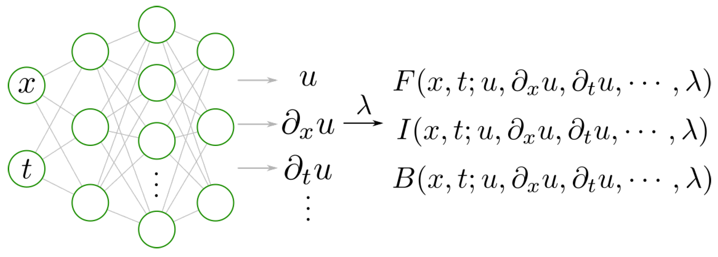
We consider a scalar function on the domain ; with the boundary , where . satisfies the following PDE (Equation (4)):
where F contains a sequence of differential operators (i.e., ), which represents the residual of the PDEs; is the PDEs’ parameter vector; I is the residual form of the initial condition containing a function ; and B is the residual form of the boundary condition containing a function . , , and .
Figure 1 illustrates the structure of a PINN model. The space coordinates x and time t are usually taken as the inputs, and the outputs are used to approximate the true solution of the PDEs. The differential operators are calculated by automatic differentiation (AD), and then the PDEs’ residuals, initial conditions, and boundary conditions are embedded into the loss function of neural networks (Equation (5)):
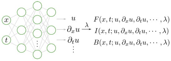
Figure 1.
PINN model.
With representing the weights of neural network; , , and are the weights for various loss terms; and , , and are the loss functions of PDE (Equation (6)), initial condition (Equation (7)), and boundary condition (Equation (8)), respectively:
where , , and are the sets of collocation points in U, , and ; and , , and denote the number of sampling points. In this manuscript, the total loss function is represented as .
After the formulation of these loss terms, the PINN can be trained using any optimizer, such as Adam, Stochastic Gradient descent, or a Netwon-based method like L-BFGS. In this work, we mainly use Adam [47] and LBFGS [48], which are described in detail in the following sections.
2.2. Optimizers
Here, we outline the common optimization algorithms used to train neural networks and to minimize the loss function.
2.2.1. Adam Optimizer
The Adam optimization algorithm is an extension to stochastic gradient descent [47]. Its core idea is to compute individual adaptive learning rates for different parameters from the estimations of the first and second moments of the gradients. The detailed computing steps are given as Algorithm 1.
| Algorithm 1 Adam Optimization | |
| Input: parameters, learning_rate, , , | |
| ▹ Initialize 1st moment vector | |
| ▹ Initialize 2nd moment vector | |
| ▹ Initialize timestep | |
| while not converged do | |
| ▹ Compute gradient of the objective function | |
| ▹ Update biased first moment estimate | |
| ▹ Update biased second raw moment estimate | |
| ▹ Bias-corrected first moment estimate | |
| ▹ Bias-corrected second moment estimate | |
| ▹ Update parameters | |
| end while | |
2.2.2. LBFGS Optimizer
Broyden–Fletcher–Goldfarb–Shanno is a quasi-Newton-based optimization algorithm commonly used for training neural networks. The loss landscape of a PINN is highly complex due to competing loss terms, making BFGS an effective choice for training PINNs.
BFGS [49] is a gradient method that iteratively computes the Hessian matrix of the loss function, and this process requires gradient evaluations, where n represents the number of parameters. The BFGS curvature matrix can be updated without the need for matrix inversion, and this reduces the computational cost significantly. However, since the Hessian matrix is the foundation of the BFGS algorithm, memory usage increases as the square of the number of parameters. This results in rapid memory usage growth, making it impractical to use this approach for neural networks with a large number of parameters. The implementation of BFGS algorithm is referred to Algorithm 2.
The BFGS algorithm may use large amounts of memory, but L-BFGS [50] solves this issue by storing a few vectors that represent an estimate of the full Hessian matrix. Compared to BFGS, L-BFGS is more computationally efficient, uses less memory, and can handle problems with larger numbers of parameters. Due to its lower memory requirements, the L-BFGS algorithm has become the favourite among second-order optimization techniques.
| Algorithm 2 BFGS Method |
|
2.3. Evaluation Metric
The approximate solution provided by the PINN needs to be evaluated and compared with the analytical solution/finite modelling result using some metric. The error between the ground truth and the approximation can be challenging to quantify. We use relative norm error (see Equation (9)).
It is used in linear algebra and defines the relative norm error. We take a discrete sample of data points from the solution space and the approximation space and store them as vectors x and b, respectively. We then find the Euclidean distance of the difference between the solution and the approximation vectors relative to the Euclidean distance of the solution.
3. Results and Discussion
To illustrate the effectiveness of PINNs in addressing high-frequency and multi-scale problems, we examined their performance on the damped harmonic oscillator problem and the 1D wave equation, both of which present unique challenges. The damped harmonic oscillator was a straightforward example of how PINNs function and where their limitations lie. Notably, while the simple harmonic oscillator followed an ordinary differential equation (ODE), the 1D wave equation represents a second-order partial differential equation. Through these examples, we aimed to showcase the versatility of PINNs in modelling both ODEs and PDEs.
3.1. Simple Harmonic Oscillator (SHM)
The damped harmonic oscillator is a classic problem in mechanics that describes the motion of a mechanical oscillator (e.g., a spring pendulum) under the influence of a restoring force and friction. The governing equation for the damped harmonic oscillator is given by Equation (10):
where
- m: mass of the oscillator;
- : coefficient of friction;
- k: spring constant.
In this paper, we focus on the under-damped state, i.e., where the oscillation is slowly damped by friction occurs when , where and .
The following initial conditions are applied:
The exact solution of the above setup is given by Equation (11):
where .
The interior residual is given by Equation (12):
This is the exact solution of the oscillator with as 20 Hz.
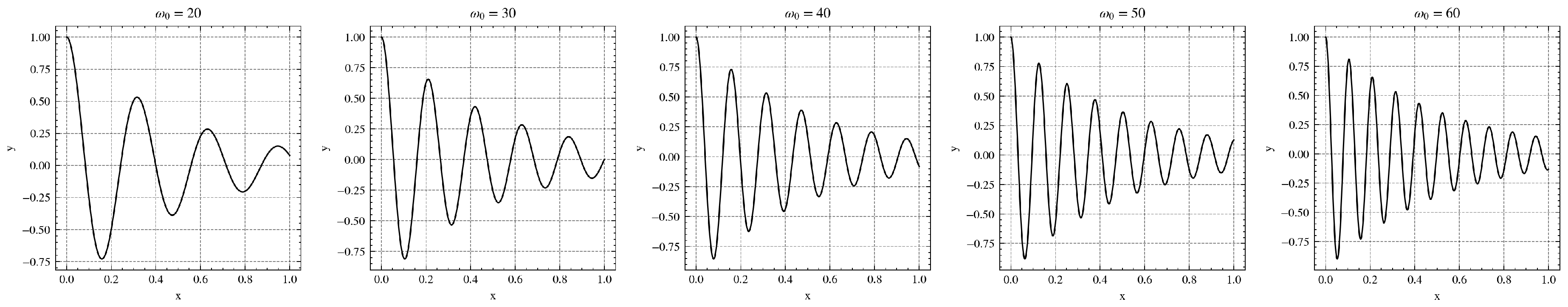
With an increasing frequency (), the damped harmonic oscillator function becomes more complicated for PINNs to approach. Figure 2 illustrates the exact solution of the oscillator for four frequencies .

Figure 2.
Exact solution for different values of .
In the experiment, our PINN model is used to approximate the solutions of the oscillator for the above four frequencies. The selected source terms yield uncomplicated solutions that demonstrate how the F-principle affects the convergence of PINNs to the numerical solution. According to the F-principle, the low-frequency or large-scale characteristics of the solution are initially manifested in the PINNs, while it may take multiple training epochs to retrieve high-frequency or small-scale features [34]. We expect that the vanilla PINN will converge faster and achieve better accuracy in learning the damped harmonic oscillator for lower-frequency components, e.g., than for higher-frequency components (). The experiment results that are presented in the following part are aligned with the expectations.
The PINN model we used in experiments for this case comprises a fully connected network (FCN) with five fully connected layers, each consisting of 64 neurons, totalling 4321 parameters. We trained the PINN model using two optimizers, Adam and L-BFGS, which are mentioned in most PINN papers. To populate the computational domain, we utilized a total of 100 equidistant points. It is worth noting that the selection of the number of points within the domain is a decision that is dependent on the user.
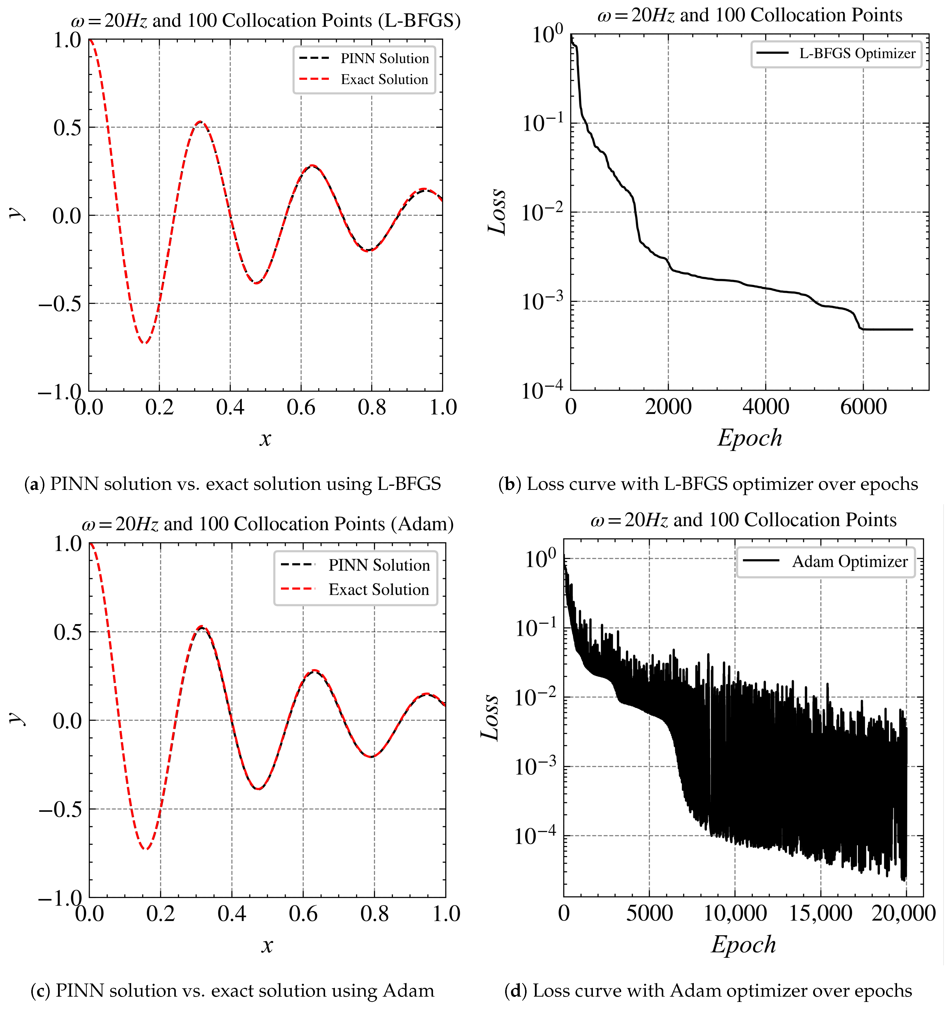
The results of training PINN models for and are given in Figure 3 and Figure 4. For , the PINN was able to fit well where the loss reaches the order of with both Adam and L-BFGS optimizers (Figure 3a,c). With the LBFGS optimizer, it converged at around 2200 epochs(Figure 3b), while with the Adam optimizer, it converged at around 7000 epochs (Figure 3d).
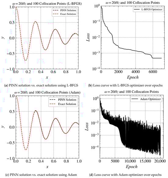
Figure 3.
Comparisons of Adam optimizer vs. L-BFGS optimizer at 20 Hz.
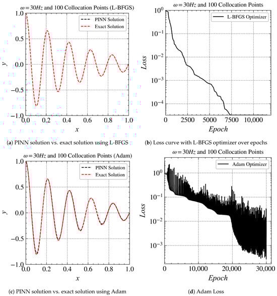
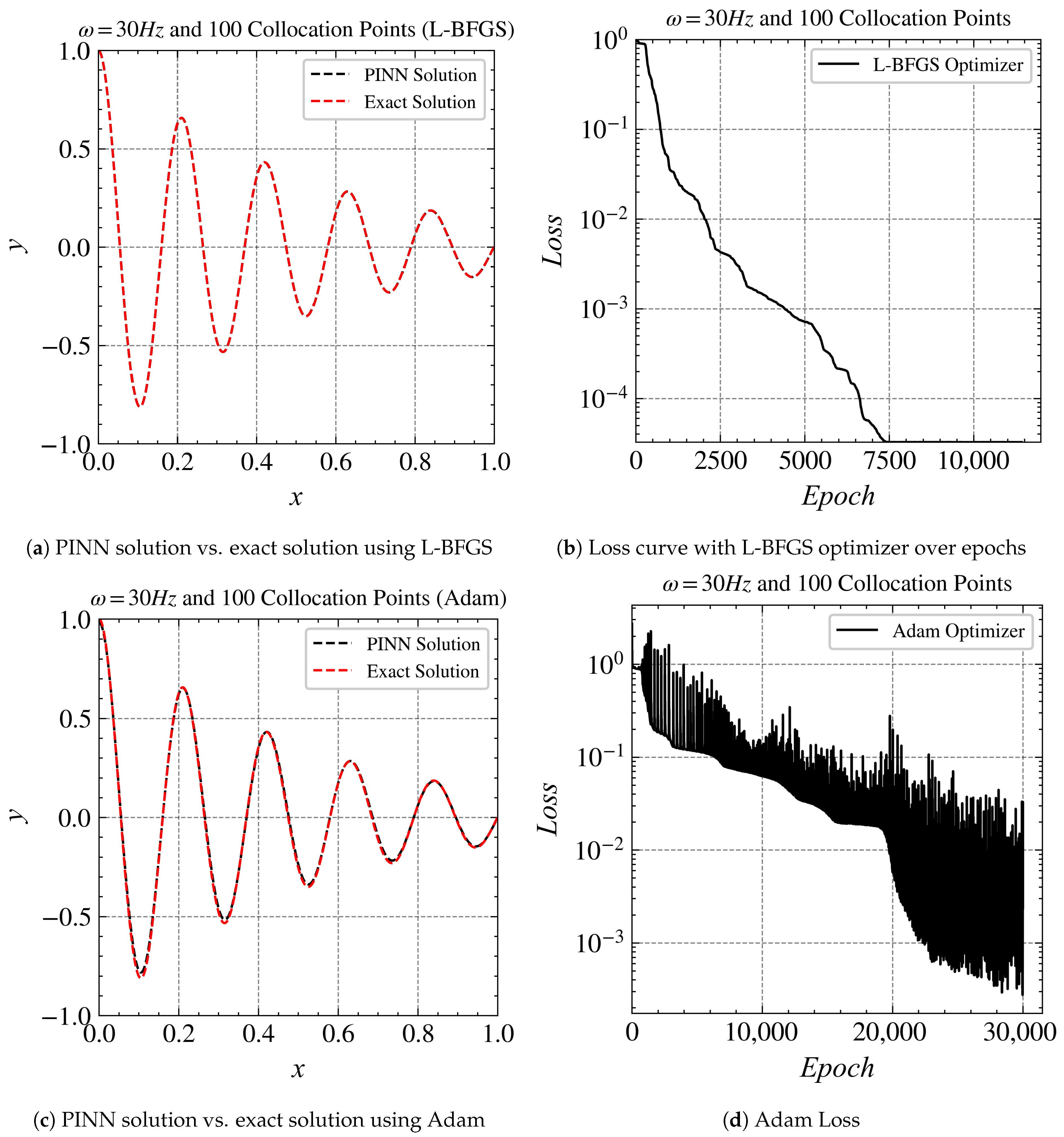
Figure 4.
Comparison of the Adam optimizer with the L-BFGS optimizer at 30 Hz: (a) comparing the PINN solution and the exact solution using L-BFGS; (b) visualization of loss curve with L-BFGS optimizer across epochs; (c) analyzing the PINN solution and exact solution using Adam; (d) loss using Adam optimizer.
For , the PINN was also able to reach the order of loss with both Adam and L-BFGS optimizers (Figure 3c and Figure 4a). With the L-BFGS optimizer, it converged at around 7000 epochs (Figure 4b). The Adam optimizer needs around 22,000 epochs to converge (Figure 4d).
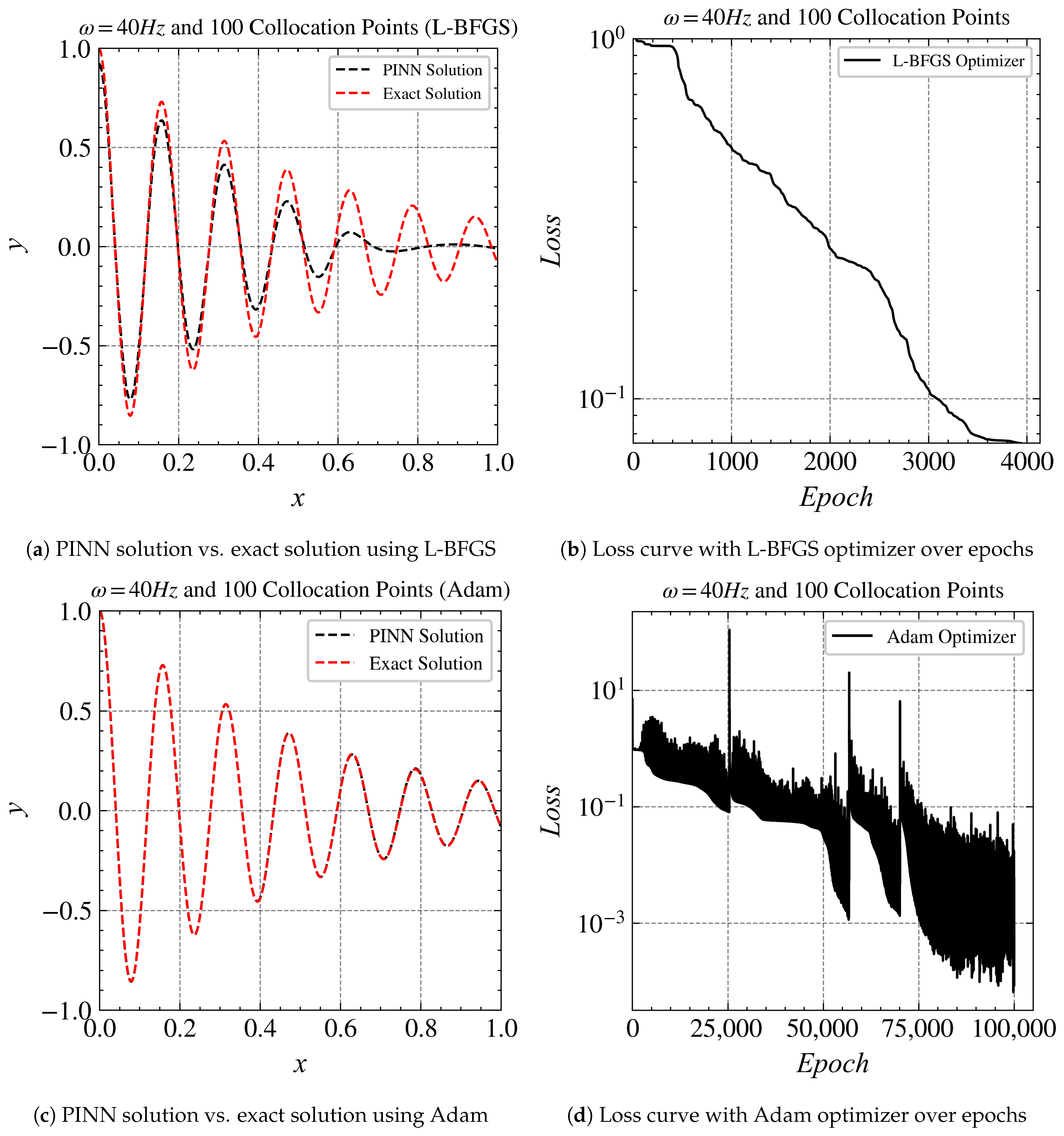
In comparing the convergence behaviour of the Adam optimizer and the L-BFGS optimizer at a frequency of 40 Hz, it becomes apparent that both algorithms exhibit different characteristics and performances, particularly in their speed of convergence and stability during optimization. The Adam optimizer eventually converges; however, this is achieved after a significant number of iterations. This observation raises concerns as we transition to higher frequencies, suggesting challenges in PINN convergence. This could be partly attributed to the well-documented issue of spectral bias inherent in neural networks.
When considering which optimizer to use, it is crucial to select one with caution as they can have a significant impact on the efficiency of the training process. We found out that using Adam with L-BFGS gave the best results.
The performance of the PINN is observed to be consistent in two different frequency scenarios (20 Hz and 30 Hz) when using Adam and L-BFGS. This indicates that the quality of predictions remains stable regardless of the chosen optimization algorithm. It is important to note that both optimizers ultimately achieve convergence and deliver favourable predictive outcomes; however, they exhibit notable differences in behaviour.
The Adam optimizer, although effective, requires a higher number of iterations to reach convergence and shows some degree of instability compared to the L-BFGS optimizer. At times, Adam outperforms L-BFGS, possibly due to L-BFGS temporarily getting stuck in a local minimum leading to quick convergence. In the context of the mentioned frequency scenarios, a learning rate of 0.1 was set for the L-BFGS optimizer. Since L-BFGS is a quasi-Newton method, it depends on the initial guess.
At a frequency of 40 Hz, Adam optimizer was able to solve the problem but it required significantly more number of iterations, with almost 80,000 iterations needed to reach convergence. On the other hand, LBFGS failed to converge and seemed to fit the lower-frequency components of the problem. It is important to note that the loss in this case remained at the order of , highlighting the problems of solving high-frequency cases within the PINN framework.
3.1.1. Transfer Learning
This section introduces a transfer learning technique to boost the robustness and convergence of training PINNs. Transfer learning presents a promising solution to mitigate these issues by leveraging the pre-trained model or the baseline PINN, thereby furnishing an advantageous initial guess to expedite convergence. To assess the efficacy of this technique, we conducted a series of experiments involving different optimization algorithms and compared their performances, respectively. The baseline low-frequency model is required to initiate the transfer learning of PINNs from low frequency to high frequency. The models mentioned in the previous part are selected for transfer learning to facilitate the scaling of the model to higher frequencies. The baseline model is established, revealing that as the frequency is elevated, the capability of the PINN, given the present configuration, to scale effectively diminishes. It is important to note that LBFGS, a Newton-based optimization method, exhibits sensitivity to the initial guess, rendering it susceptible to convergence challenges, including the risk of getting trapped in local minima or failing to converge even after a substantial number of iterations. Some empirical evidence shows that Adam optimizer when used with a combination of the L-BFGS optimizer, ensures that the latter escapes from the local minima [34]. We selected the baseline models at 30 Hz generated by both the Adam and LBFGS optimizers. These models were subsequently employed as the starting point for training a PINN model targeting a frequency of 40 Hz. This approach enables us to evaluate which of the two optimizers produces a more effective baseline model for this task.
3.1.2. Discussion of Results
In this section, we test out both Adam and L-BFGS optimizers to see which of the two performs better as a source model to scale to higher frequencies. Then, the source models are trained with L-BFGS to transfer learning to the desired higher-frequency models.
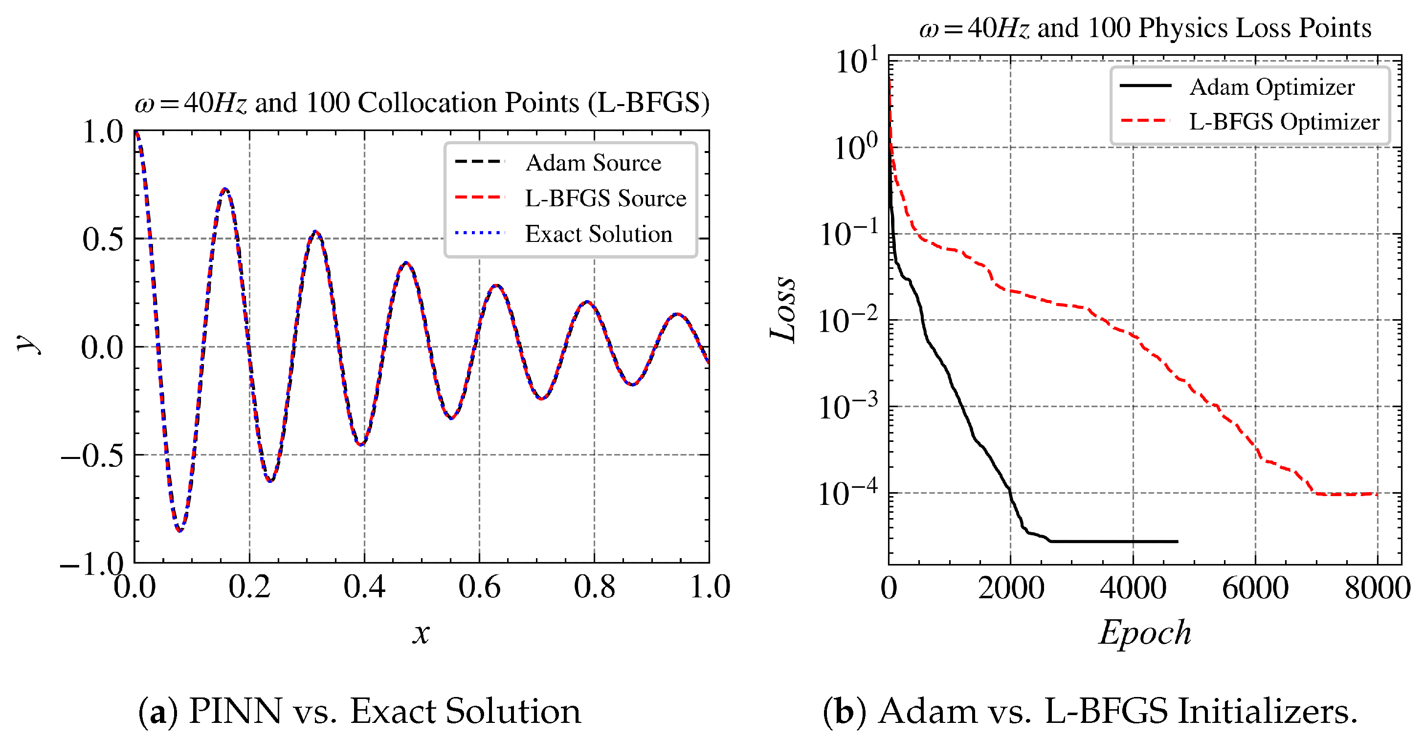
The results of the 40 Hz case without transfer learning are given in Figure 5 as a baseline. Both Adam and L-BFGS optimization algorithms are tested, leading to two versions of baseline models. In the following results, we use L-BFGS to train the network. Figure 6 shows each of the baseline model’s solutions compared to the exact solution and its training curve. We make use of transfer learning and compare it with Adam and L-BFGS baseline models. In Figure 6b, it is evident that the source model for 30 Hz with Adam performed much better than that of L-BFGS. As mentioned above, this might be due to the nature of L-BFGS.
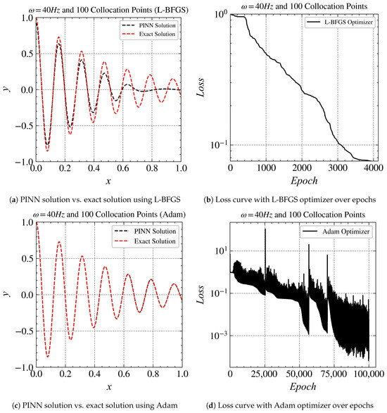
Figure 5.
Comparisons of Adam optimizer vs. L-BFGS optimizer at 40 Hz.

Figure 6.
Comparisons of 40 Hz for Adam and LBFGS.
When we compare the results of the 40 Hz case without transfer learning (Figure 5d) with those using transfer learning (Figure 6b), we observe that Adam achieved a loss order of in about 75,000 iterations, while the one using transfer learning achieved the same order in less than 2000 epochs. This not only reduced the computation time significantly but also provided a more accurate solution.
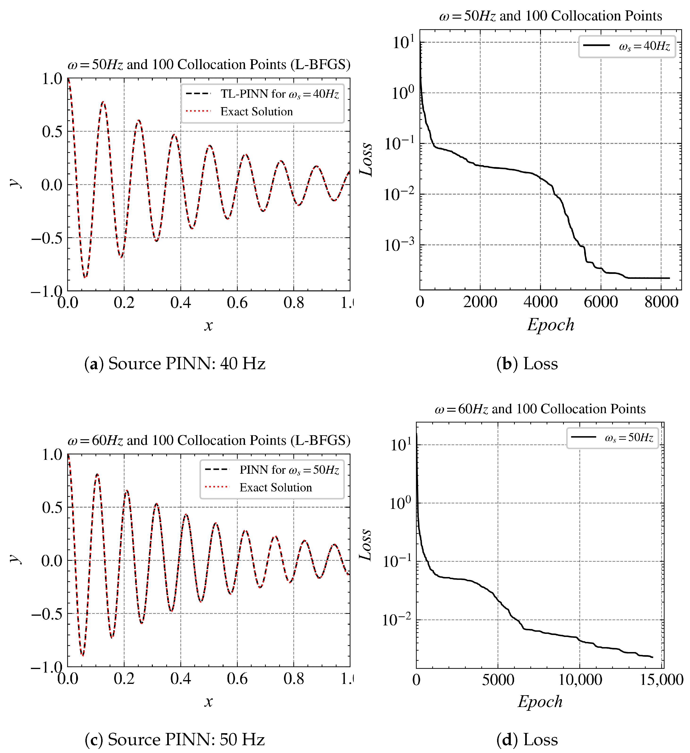
Now, moving on to the next set of results, we use the 40 Hz model as the source to train the model on . Similarly, we used the model as the source to train the model on . The results are given in Figure 7. In both cases, the L-BFGS optimizer was used to train the model. The order of loss for Hz is higher than that of Hz because of the complexity of the solution; however, the PINN’s solutions fit well with the exact solution. By comparing the relative L2 error as described in Table 1, we can conclude that although LBFGS performs more stably than Adam in training the initial model, it does not provide a “good” initial model for transferring to higher-frequency problems. It is difficult for Adam to handle high-frequency problems, but it provides better initial models on low-frequency problems. Using transfer learning to transfer the model trained with Adam from low-frequency problems to high-frequency problems obtain more accurate solutions.
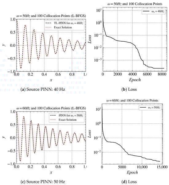
Figure 7.
Transfer learning results for Hz and Hz. In both the cases, L-BFGS optimizer was used to train the model. The order of loss for Hz is higher than that that of Hz because of the complexity of the solution; however, the PINN’s solutions fit well with the exact solution.

Table 1.
Relative L2 error (%).
3.2. One-Dimensional Wave Equation
The wave equation (Equation (13)):
models the oscillations of a one-dimensional string (), the oscillations of a two-dimensional thin membrane (), or the pressure oscillations of an acoustic wave in air (). The constant c denotes the velocity of wave propagation for the oscillations and is also known as the wave velocity in certain literature studies.
Although typically discussed in just one spatial dimension (x) due to time (t) being the only independent variable, it is important to mention that the variable we are studying (u) can represent movement in another direction, like up and down (y). For example, this occurs when a string is not only moving horizontally (x) but also vertically (y), as seen on a flat surface.
The unknown function u depends on space x and time t, and can be represented as an equation
We also need initial conditions and boundary conditions to solve the function. In the experiments, we use the conditions given in Equation (14):
We solve the case where . Specifically, we address the equation with homogeneous Dirichlet conditions, , and compare the results with the analytical solution.
As we increase c from 1 to 2, we observe that the solution takes much longer to converge. To address this, we employ transfer learning. We first train the model for and then use this knowledge to approximate the solution for .
To do so, we approximate the underlying solution with a feedforward dense neural network with tunable parameters :
This approach allows us to efficiently model and compare solutions under different conditions, providing a deeper understanding of the system’s behaviour.
The spatial boundary residual or boundary conditions are given by Equation (16):
The temporal boundary residual is given by Equation (17):
With the training input points corresponding to low-discrepancy Sobol sequences, the loss terms are given in Equations (18)–(20):
where is the number of collocation points or the PDE points; represents each spatial boundary or boundary condition points; and is either the temporal boundary points or the initial condition points.
Finally, we train our neural network to minimize the above loss terms and find the parameter (Equation (21)):
The weight () for the temporal loss term is given by the Equation (22):
where
- -
- is the weight for the temporal loss term;
- -
- is a constant;
- -
- t is the current time;
- -
- is the maximum time.
In the first experiments, we added an approximation of the wave for c = 1. We know the exact solution for that case, which is (Equation (23)):
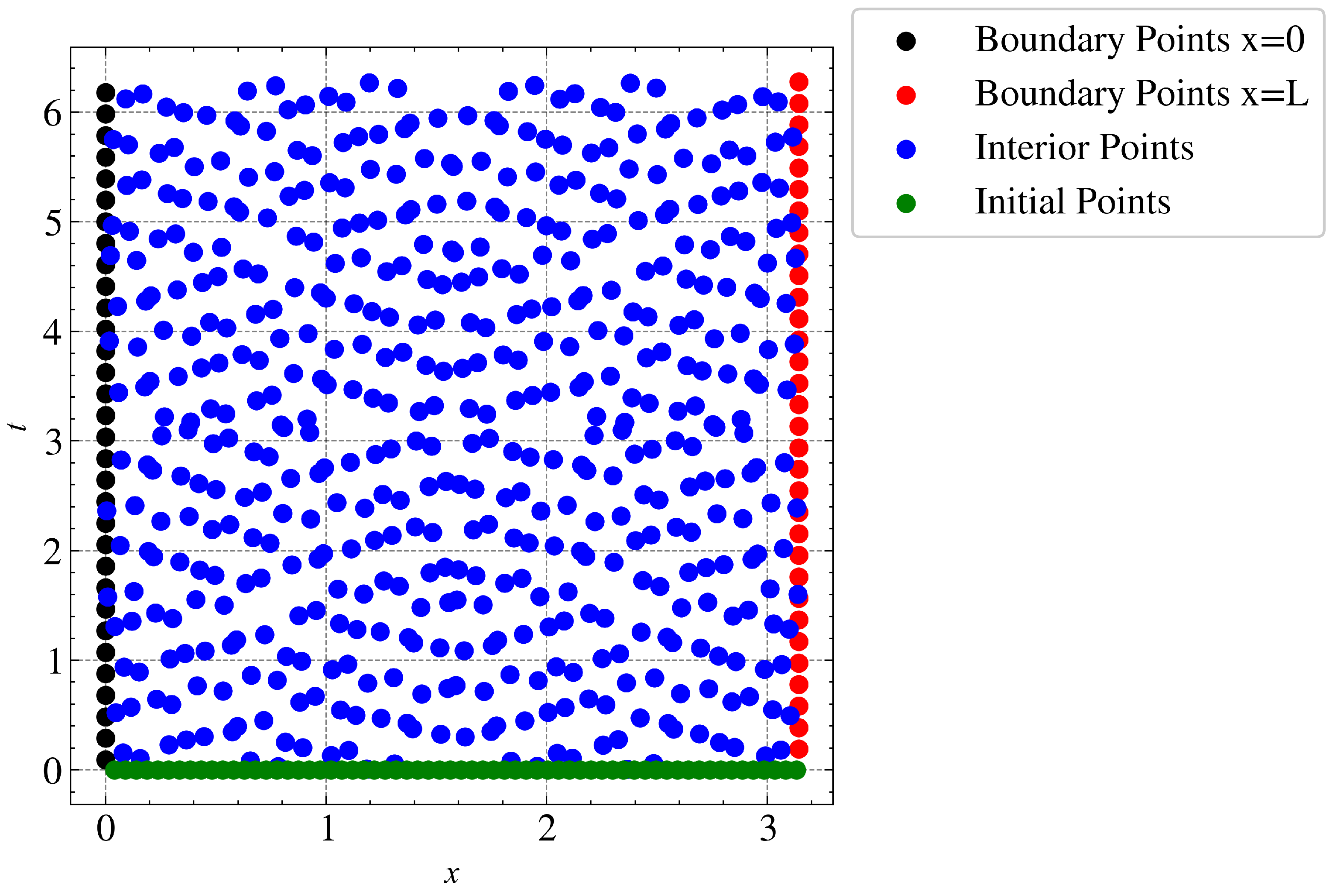
For this experiment, we used a fully connected neural network comprising five layers and 64 units. Sobol sequences were used to generate collocation points, spatial boundary points and temporal boundary points. Figure 8 shows an example of the corresponding points sampled from the studied domain. Specifically, we generated 512 collocation points, 32 temporal points, and 64 points on each boundary. The network was optimized using an L-BFGS optimizer.
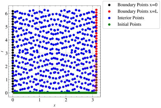
Figure 8.
Sampled points over the spatial and temporal domains. At x = 0 and x = L, boundary points are added, which will define the value that will take.
Results for 1D Wave Equation
For c = 1, the L2 relative error norm between the exact solution and PINN solution is 0.05%.
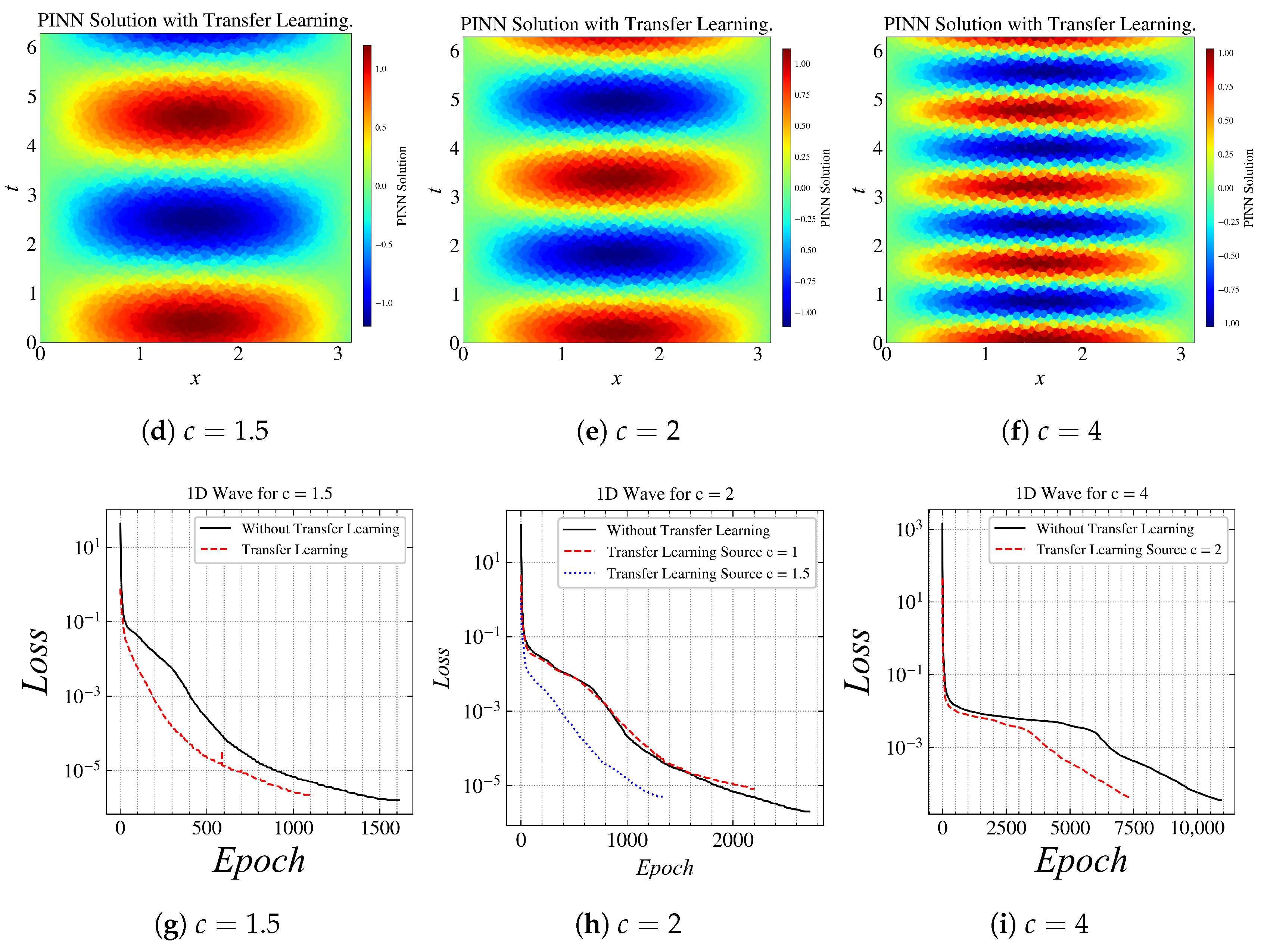
Figure 9 compactly shows the baseline model and the training results of using transfer learning to train PINN to solve higher frequency problems. The result in Figure 9a is the baseline or the source model that we trained, for c = 1. Now, in the upcoming results, we use this model as a source; as we increase the value of c to 1.5, 2.0, and 4.0. The model that used transfer learning performed better than the models without transfer learning. In Figure 9g, the loss reached an order of in 600 epochs with transfer learning, whereas it took 1000 epochs without transfer learning. Figure 9h,i show the consistent results that the loss reached an order of in fewer epochs with transfer learning.
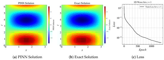
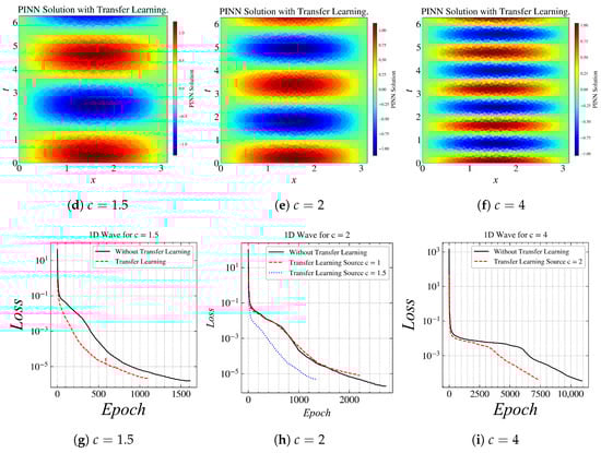
Figure 9.
Results for (L-BFGS): (a) approximated solution by PINN, (b) exact solution, (c) loss curve. Results for various values of c with transfer learning: (d) , (e) , (f) . Loss curves for: (g) , (h) , (i) .
It can be observed in Figure 9i that the model without transfer learning took more than 10,000 epochs to converge, whereas the model which used transfer learning took only 7500 epochs to converge. The order of loss is not as low as the other results because of the complexity of the solution.
4. Conclusions
This work aims to shed light on the common challenges encountered by PINNs when applied to high-frequency and multi-scale problems. We explored the potential of transfer learning as a viable solution to these problems. In the experiments, we observed that the PINN depicts ability in approximating the harmonic oscillator at a frequency of 20 Hz. However, as the frequency increases, a noticeable increase in computational cost follows, accompanied by increased convergence times.
The application of the vanilla PINN, utilizing an identical neural network architecture as the 20 Hz case, proves unfeasible in achieving convergence at 40 Hz, 50 Hz, and 60 Hz with the same amount of collocation points. While the model performs well on low-frequency problems, it starts struggling when given higher frequencies. Through transfer learning, we were able to learn the 50 Hz and 60 Hz solutions, without adding more layers, or changing the number of collocation points. The results were promising as well, with a loss reaching an order of .
Similarly, in the context of the one-dimensional wave equation, with the use of transfer learning, we learnt the PINN solution for different wave velocities, starting from two up to four. The transfer learning method turned out to be effective. As for a higher wave velocity, the model achieved convergence significantly quicker.
Transfer learning has proven to be an effective method for enhancing the efficiency and convergence characteristics of PINNs, preventing the necessity for modifications to the network architecture, which causes more parameters. A meaningful research direction is establishing a pre-trained model library for complex engineering problems so that transfer learning technology can be used to train models for specific problems rapidly and accurately.
However, applying transfer learning techniques is not without its pitfalls. Negative transfer describes the phenomenon where inappropriately transferring knowledge from the source domain can inversely hurt the target performance [51]. Although we did not observe any negative effects resulting from the application of transfer learning in the experiments involved in this article, this does not mean that the technique can be applied to the training of PINNs without careful consideration. The important point here is to understand the limitations of transfer learning, that is, under what circumstances transfer learning might fail, and how such failures can be avoided. We believe this contributes not only to the theory of PINN training but also has practical significance in solving more complex real-world engineering problems. This also points to the direction of our future work.
Author Contributions
Conceptualization, H.L. and Z.R.; methodology, A.H.M., H.L. and F.W.; software, A.H.M. and H.L.; validation, A.H.M. and H.L.; formal analysis, A.H.M. and H.L.; investigation, A.H.M. and H.L.; data curation, A.H.M. and H.L.; writing—original draft preparation, A.H.M. and H.L.; writing—review and editing, A.H.M., H.L. and Z.R.; visualization, A.H.M. and H.L.; supervision, H.L. and Z.R.; project administration, H.L., F.W. and Z.R. All authors have read and agreed to the published version of the manuscript.
Funding
A.H.M. would like to thank the Erasmus Plus Traineeship programme offered at the University of Genova, Italy, and Kiel University for providing computational facilities. The authors acknowledge financial support by Land Schleswig-Holstein within the funding programme Open Access Publikationsfonds.
Institutional Review Board Statement
Not applicable.
Informed Consent Statement
Not applicable.
Data Availability Statement
The data points used for training PINN models can be sampled using the method mentioned in the article.
Conflicts of Interest
Author Zarghaam Rizvi was employed by the company GeoAnalysis Engineering GmbH. The remaining authors declare that the research was conducted in the absence of any commercial or financial relationships that could be construed as a potential conflict of interest.
References
- Raissi, M.; Perdikaris, P.; Karniadakis, G.E. Physics Informed Deep Learning (Part I): Data-driven Solutions of Nonlinear Partial Differential Equations. arXiv 2017, arXiv:1711.10561. [Google Scholar]
- Raissi, M.; Perdikaris, P.; Karniadakis, G.E. Physics Informed Deep Learning (Part II): Data-driven Discovery of Nonlinear Partial Differential Equations. arXiv 2017, arXiv:1711.10566. [Google Scholar]
- Raissi, M.; Perdikaris, P.; Karniadakis, G. Physics-informed neural networks: A deep learning framework for solving forward and inverse problems involving nonlinear partial differential equations. J. Comput. Phys. 2019, 378, 686–707. [Google Scholar] [CrossRef]
- Cai, S.; Mao, Z.; Wang, Z.; Yin, M.; Karniadakis, G.E. Physics-informed neural networks (PINNs) for fluid mechanics: A review. Acta Mech. Sin. 2021, 37, 1727–1738. [Google Scholar] [CrossRef]
- Wang, H.; Li, J.; Wang, L.; Liang, L.; Zeng, Z.; Liu, Y. On acoustic fields of complex scatters based on physics-informed neural networks. Ultrasonics 2023, 128, 106872. [Google Scholar] [CrossRef] [PubMed]
- Haghighat, E.; Raissi, M.; Moure, A.; Gomez, H.; Juanes, R. A physics-informed deep learning framework for inversion and surrogate modeling in solid mechanics. Comput. Methods Appl. Mech. Eng. 2021, 379, 113741. [Google Scholar] [CrossRef]
- Liang, R.; Liu, W.; Xu, L.; Qu, X.; Kaewunruen, S. Solving elastodynamics via physics-informed neural network frequency domain method. Int. J. Mech. Sci. 2023, 258, 108575. [Google Scholar] [CrossRef]
- Rao, C.; Sun, H.; Liu, Y. Physics-Informed Deep Learning for Computational Elastodynamics without Labeled Data. J. Eng. Mech. 2021, 147, 04021043. [Google Scholar] [CrossRef]
- Zhou, M.; Mei, G. Transfer Learning-Based Coupling of Smoothed Finite Element Method and Physics-Informed Neural Network for Solving Elastoplastic Inverse Problems. Mathematics 2023, 11, 2529. [Google Scholar] [CrossRef]
- Okazaki, T.; Ito, T.; Hirahara, K.; Ueda, N. Physics-informed deep learning approach for modeling crustal deformation. Nat. Commun. 2022, 13, 7092. [Google Scholar] [CrossRef]
- Rasht-Behesht, M.; Huber, C.; Shukla, K.; Karniadakis, G.E. Physics-Informed Neural Networks (PINNs) for Wave Propagation and Full Waveform Inversions. J. Geophys. Res. Solid Earth 2022, 127, e2021JB023120. [Google Scholar] [CrossRef]
- Karimpouli, S.; Tahmasebi, P. Physics informed machine learning: Seismic wave equation. Geosci. Front. 2020, 11, 1993–2001. [Google Scholar] [CrossRef]
- Krishnapriyan, A.; Gholami, A.; Zhe, S.; Kirby, R.; Mahoney, M.W. Characterizing possible failure modes in physics-informed neural networks. In Proceedings of the Advances in Neural Information Processing Systems, Virtual, 6–14 December 2021; Ranzato, M., Beygelzimer, A., Dauphin, Y., Liang, P., Vaughan, J.W., Eds.; Neural Information Processing Systems Foundation, Inc. (NeurIPS): San Diego, CA, USA, 2021; Volume 34, pp. 26548–26560. [Google Scholar]
- Wang, S.; Teng, Y.; Perdikaris, P. Understanding and Mitigating Gradient Flow Pathologies in Physics-Informed Neural Networks. SIAM J. Sci. Comput. 2021, 43, A3055–A3081. [Google Scholar] [CrossRef]
- Rahaman, N.; Baratin, A.; Arpit, D.; Draxler, F.; Lin, M.; Hamprecht, F.; Bengio, Y.; Courville, A. On the Spectral Bias of Neural Networks. In Proceedings of the 36th International Conference on Machine Learning, Long Beach, CA, USA, 10–15 June 2019; Chaudhuri, K., Salakhutdinov, R., Eds.; PMLR: Cambridge, MA, USA, 2019; Volume 97, pp. 5301–5310. [Google Scholar]
- Cao, Y.; Fang, Z.; Wu, Y.; Zhou, D.X.; Gu, Q. Towards Understanding the Spectral Bias of Deep Learning. In Proceedings of the Thirtieth International Joint Conference on Artificial Intelligence (IJCAI 2021), Virtual, 19–26 August 2021; Zhou, Z.H., Ed.; pp. 2205–2211. [Google Scholar] [CrossRef]
- Waheed, U.B. Kronecker Neural Networks Overcome Spectral Bias for PINN-Based Wavefield Computation. IEEE Geosci. Remote Sens. Lett. 2022, 19, 1–5. [Google Scholar] [CrossRef]
- Wang, S.; Wang, H.; Perdikaris, P. On the eigenvector bias of Fourier feature networks: From regression to solving multi-scale PDEs with physics-informed neural networks. Comput. Methods Appl. Mech. Eng. 2021, 384, 113938. [Google Scholar] [CrossRef]
- Tancik, M.; Srinivasan, P.; Mildenhall, B.; Fridovich-Keil, S.; Raghavan, N.; Singhal, U.; Ramamoorthi, R.; Barron, J.; Ng, R. Fourier Features Let Networks Learn High Frequency Functions in Low Dimensional Domains. In Proceedings of the Advances in Neural Information Processing Systems, Virtual, 6–12 December 2020; Larochelle, H., Ranzato, M., Hadsell, R., Balcan, M., Lin, H., Eds.; Neural Information Processing Systems Foundation, Inc. (NeurIPS): San Diego, CA, USA, 2020; Volume 33, pp. 7537–7547. [Google Scholar]
- Kollmannsberger, S.; Singh, D.; Herrmann, L. Transfer Learning Enhanced Full Waveform Inversion. arXiv 2023, arXiv:2302.11259. [Google Scholar]
- Yang, F.; Ma, J. FWIGAN: Full-Waveform Inversion via a Physics-Informed Generative Adversarial Network. J. Geophys. Res. Solid Earth 2023, 128, e2022JB025493. [Google Scholar] [CrossRef]
- Yang, F.; Ma, J. Wasserstein Distance-Based Full-Waveform Inversion With a Regularizer Powered by Learned Gradient. IEEE Trans. Geosci. Remote Sens. 2023, 61, 5904813. [Google Scholar] [CrossRef]
- Muller, A.P.O.; Costa, J.C.; Bom, C.R.; Klatt, M.; Faria, E.L.; de Albuquerque, M.P.; de Albuquerque, M.P. Deep pre-trained FWI: Where supervised learning meets the physics-informed neural networks. Geophys. J. Int. 2023, 235, 119–134. [Google Scholar] [CrossRef]
- Alkhadhr, S.; Almekkawy, M. Modeling the Wave Equation Using Physics-Informed Neural Networks Enhanced With Attention to Loss Weights. In Proceedings of the ICASSP 2023—2023 IEEE International Conference on Acoustics, Speech and Signal Processing (ICASSP), Rhodes Island, Greece, 4–10 June 2023; pp. 1–5. [Google Scholar] [CrossRef]
- Alkhadhr, S.; Almekkawy, M. Wave Equation Modeling via Physics-Informed Neural Networks: Models of Soft and Hard Constraints for Initial and Boundary Conditions. Sensors 2023, 23, 2792. [Google Scholar] [CrossRef]
- Nguyen, H.; Tsai, R. Numerical wave propagation aided by deep learning. J. Comput. Phys. 2023, 475, 111828. [Google Scholar] [CrossRef]
- Maczuga, P.; Paszyński, M. Influence of Activation Functions on the Convergence of Physics-Informed Neural Networks for 1D Wave Equation. In Proceedings of the Computational Science—ICCS 2023; Mikyška, J., de Mulatier, C., Paszynski, M., Krzhizhanovskaya, V.V., Dongarra, J.J., Sloot, P.M., Eds.; Springer: Cham, Switzerland, 2023; pp. 74–88. [Google Scholar]
- Pan, S.J.; Yang, Q. A Survey on Transfer Learning. IEEE Trans. Knowl. Data Eng. 2010, 22, 1345–1359. [Google Scholar] [CrossRef]
- Tripuraneni, N.; Jordan, M.; Jin, C. On the Theory of Transfer Learning: The Importance of Task Diversity. In Proceedings of the Advances in Neural Information Processing Systems, Virtual, 6–12 December 2020; Larochelle, H., Ranzato, M., Hadsell, R., Balcan, M., Lin, H., Eds.; Neural Information Processing Systems Foundation, Inc. (NeurIPS): San Diego, CA, USA, 2020; Volume 33, pp. 7852–7862. [Google Scholar]
- Phung, T.; Le, T.; Vuong, T.L.; Tran, T.; Tran, A.; Bui, H.; Phung, D. On Learning Domain-Invariant Representations for Transfer Learning with Multiple Sources. In Proceedings of the Advances in Neural Information Processing Systems, Virtual, 6–14 December 2021; Ranzato, M., Beygelzimer, A., Dauphin, Y., Liang, P., Vaughan, J.W., Eds.; Curran Associates, Inc.: Red Hook, NY, USA, 2021; Volume 34, pp. 27720–27733. [Google Scholar]
- Neyshabur, B.; Sedghi, H.; Zhang, C. What is being transferred in transfer learning? In Proceedings of the Advances in Neural Information Processing Systems, Virtual, 6–12 December 2020; Larochelle, H., Ranzato, M., Hadsell, R., Balcan, M., Lin, H., Eds.; Neural Information Processing Systems Foundation, Inc. (NeurIPS): San Diego, CA, USA, 2020; Volume 33, pp. 512–523. [Google Scholar]
- Tajbakhsh, N.; Shin, J.Y.; Gurudu, S.R.; Hurst, R.T.; Kendall, C.B.; Gotway, M.B.; Liang, J. Convolutional Neural Networks for Medical Image Analysis: Full Training or Fine Tuning? IEEE Trans. Med Imaging 2016, 35, 1299–1312. [Google Scholar] [CrossRef] [PubMed]
- Deng, Z.; Zhang, L.; Vodrahalli, K.; Kawaguchi, K.; Zou, J.Y. Adversarial Training Helps Transfer Learning via Better Representations. In Proceedings of the Advances in Neural Information Processing Systems, Virtual, 6–14 December 2021; Ranzato, M., Beygelzimer, A., Dauphin, Y., Liang, P., Vaughan, J.W., Eds.; Curran Associates, Inc.: Red Hook, NY, USA, 2021; Volume 34, pp. 25179–25191. [Google Scholar]
- Markidis, S. The Old and the New: Can Physics-Informed Deep-Learning Replace Traditional Linear Solvers? Front. Big Data 2021, 4, 669097. [Google Scholar] [CrossRef] [PubMed]
- Prantikos, K.; Chatzidakis, S.; Tsoukalas, L.H.; Heifetz, A. Physics-informed neural network with transfer learning (TL-PINN) based on domain similarity measure for prediction of nuclear reactor transients. Sci. Rep. 2023, 13, 16840. [Google Scholar] [CrossRef] [PubMed]
- Xu, C.; Cao, B.T.; Yuan, Y.; Meschke, G. Transfer learning based physics-informed neural networks for solving inverse problems in engineering structures under different loading scenarios. Comput. Methods Appl. Mech. Eng. 2023, 405, 115852. [Google Scholar] [CrossRef]
- Tang, H.; Liao, Y.; Yang, H.; Xie, L. A transfer learning-physics informed neural network (TL-PINN) for vortex-induced vibration. Ocean Eng. 2022, 266, 113101. [Google Scholar] [CrossRef]
- Chakraborty, S. Transfer learning based multi-fidelity physics informed deep neural network. J. Comput. Phys. 2021, 426, 109942. [Google Scholar] [CrossRef]
- Goswami, S.; Anitescu, C.; Chakraborty, S.; Rabczuk, T. Transfer learning enhanced physics informed neural network for phase-field modeling of fracture. Theor. Appl. Fract. Mech. 2020, 106, 102447. [Google Scholar] [CrossRef]
- Chen, J.; Gildin, E.; Killough, J.E. Transfer learning-based physics-informed convolutional neural network for simulating flow in porous media with time-varying controls. arXiv 2023, arXiv:2310.06319. [Google Scholar]
- Anitescu, C.; İsmail Ateş, B.; Rabczuk, T. Physics-Informed Neural Networks: Theory and Applications. In Machine Learning in Modeling and Simulation: Methods and Applications; Rabczuk, T., Bathe, K.J., Eds.; Springer: Cham, Switzerland, 2023; pp. 179–218. [Google Scholar] [CrossRef]
- Baydin, A.G.; Pearlmutter, B.A.; Radul, A.A.; Siskind, J.M. Automatic differentiation in machine learning: A survey. J. Mach. Learn. Res. 2018, 18, 5595–5637. [Google Scholar]
- Lu, L.; Meng, X.; Mao, Z.; Karniadakis, G.E. DeepXDE: A Deep Learning Library for Solving Differential Equations. SIAM Rev. 2021, 63, 208–228. [Google Scholar] [CrossRef]
- Hennigh, O.; Narasimhan, S.; Nabian, M.A.; Subramaniam, A.; Tangsali, K.; Fang, Z.; Rietmann, M.; Byeon, W.; Choudhry, S. NVIDIA SimNet™: An AI-Accelerated Multi-Physics Simulation Framework. In Proceedings of the Computational Science—ICCS 2021, Krakow, Poland, 16–18 June 2021; Paszynski, M., Kranzlmüller, D., Krzhizhanovskaya, V.V., Dongarra, J.J., Sloot, P.M., Eds.; Springer: Cham, Switzerland, 2021; pp. 447–461. [Google Scholar]
- Haghighat, E.; Juanes, R. SciANN: A Keras/TensorFlow wrapper for scientific computations and physics-informed deep learning using artificial neural networks. Comput. Methods Appl. Mech. Eng. 2021, 373, 113552. [Google Scholar] [CrossRef]
- LeCun, Y.; Bengio, Y.; Hinton, G. Deep learning. Nature 2015, 521, 436–444. [Google Scholar] [CrossRef] [PubMed]
- Kingma, D.P.; Ba, J. Adam: A method for stochastic optimization. arXiv 2014, arXiv:1412.6980. [Google Scholar]
- Byrd, R.H.; Lu, P.; Nocedal, J.; Zhu, C. A Limited Memory Algorithm for Bound Constrained Optimization. SIAM J. Sci. Comput. 1995, 16, 1190–1208. [Google Scholar] [CrossRef]
- Nocedal, J.; Wright, S. Numerical Optimization; Springer Series in Operations Research and Financial Engineering; Springer Nature: Berlin/Heidelberg, Germany, 2006; pp. 1–664. [Google Scholar]
- Liu, D.C.; Nocedal, J. On the limited memory BFGS method for large scale optimization. Math. Program. 1989, 45, 503–528. [Google Scholar] [CrossRef]
- Wang, Z.; Dai, Z.; Poczos, B.; Carbonell, J. Characterizing and Avoiding Negative Transfer. In Proceedings of the IEEE/CVF Conference on Computer Vision and Pattern Recognition (CVPR), Long Beach, CA, USA, 15–20 June 2019. [Google Scholar]

Disclaimer/Publisher’s Note: The statements, opinions and data contained in all publications are solely those of the individual author(s) and contributor(s) and not of MDPI and/or the editor(s). MDPI and/or the editor(s) disclaim responsibility for any injury to people or property resulting from any ideas, methods, instructions or products referred to in the content. |
© 2024 by the authors. Licensee MDPI, Basel, Switzerland. This article is an open access article distributed under the terms and conditions of the Creative Commons Attribution (CC BY) license (https://creativecommons.org/licenses/by/4.0/).