Abstract
This study aimed to solve the problem that is the frequent switching between the acceleration and braking modes of the driverless ferry vehicle, affecting the comfort and stability of speed control. The driverless ferry vehicle encounters unknown obstacles on the road that affect the normal planning and tracking control of the ferry vehicle and finally lead to the problem that the driverless ferry vehicle cannot drive normally. First of all, in the longitudinal control, the fuzzy PID control algorithm was utilized to produce the fuzzy PID acceleration controller by taking into account the difference between the actual and expected speeds and choosing the triangular membership function. According to the relationship between the brake oil pressure and brake torque, the brake controller was designed. The acceleration/braking switching module with acceleration tolerance zone was added to the longitudinal controller, and the acceleration/braking mode-switching controller was designed. Secondly, in the lateral control, the tire cornering stiffness was analyzed, an MPC controller with a planning module was designed, and a lateral motion controller with an obstacle avoidance replanning function was proposed. Finally, according to the prediction time domain of different planning modules corresponding to different speeds, a coordinated control strategy of horizontal and longitudinal motion was proposed by using a real-time speed adjustment planning module to predict the time domain. Through the joint simulation analysis of MATLAB and CarSim, the results show that the driving stability of the ferry vehicle was significantly improved, and the longitudinal speed error of the ferry vehicle was reduced by 43.59%. The ferry’s avoidance of obstacles and tracking of reference trajectories were significantly improved, so that the tracking error can be reduced by 61.11%.
1. Introduction
The casualties and economic losses caused by road traffic accidents are increasing year by year. In the face of such serious traffic safety problems, it is urgent to improve automobile safety performance. Intelligent vehicles, with their capacity to reduce traffic accidents, enhance transport efficiency, and offer promising market prospects, have garnered significant attention. They hold the potential to drive forward the future of the automotive industry [1]. Self-driving technology is the key technology of vehicle active safety, which can effectively reduce the loss of personnel and property caused by traffic accidents. A good control algorithm is the premise of obstacle avoidance and trajectory tracking in a driverless vehicle. Researchers, both domestically and internationally, have extensively investigated this topic. To address the problem of path planning and trajectory tracking, Li et al. [2] used adaptive dynamic planning (ADP) and the APF method to solve the dynamic path planning problem. It has been proven that this method can plan the obstacle avoidance path in both dynamic and static environments. To improve the safety of the planned obstacle avoidance paths, Li et al. [3] proposed a novel path-planning approach utilizing enhanced genetic algorithms and dynamic window methods. Gao et al. [4] proposed an adaptive model predictive controller through fuzzy adaptive control methods to achieve the adaptive optimization of the weights of the objective function in the model predictive, aiming to enhance control effectiveness. The trajectory tracking method based on optimal preview was mainly proposed by Macadam [5,6] and improved gradually. In this method, the vehicle is considered to be in uniform motion or a variable speed motion with slow speed change, so that the vehicle’s horizontal and vertical controls are decoupled. Path tracking is accomplished using lateral control, and speed tracking is accomplished using longitudinal control. In order to better imitate the method of a real driver’s driving, Li et al. [7] considered the multi-point preview inaccuracy of the path, designed an MPC controller using a dynamic model, and constructed an articulated vehicle model using dynamic model predictive control, which improved the stability under limited operating conditions. Li et al. [8] proposed a steering strategy based on fuzzy logic to realize parameter self-adjustment based on displacement error to make its trajectory tracking more stable and accurate. In order to improve the parameter uncertainty of the bicycle model, Guo et al. [9] designed a longitudinal controller based on adaptive estimation of dynamic surfaces through a neural network. The experimental data show that the controller drives safely within the operation limit of the vehicle. Tang et al. [10] investigated the utilization of fuzzy controllers and model predictive controllers in intelligent vehicle trajectory tracking control. And on this basis, the PSO algorithm was used to study the parameter optimization of the prediction time domain and control time domain in the model predictive controller. Elias et al. [11] optimized the PID longitudinal speed controller. The controller has better real-time performance and tracking accuracy than the PSO algorithm-based controller. Razmjooei et al. [12] designed a reverse-tracking control based on disturbance observer, which is used to estimate and track the reference signal of electro-hydraulic actuator (EHA) system in finite time. The key idea is to use the monotone increasing function related to the control target to improve the control performance, in which Lyapunov stability analysis is used to guarantee the finite time boundedness criterion. The proposed method has higher accuracy and faster convergence. Waschl et al. [13] proposed a distributed model predictive control method for the special situation of fully autonomous vehicles in which multiple agents can pass through intersections at the same time, while maintaining a sufficient safe distance from conflicting agents. After the simulation, the study conclusively demonstrated the effectiveness of the method. Ye [14] constructed a new lateral control algorithm for driverless cars that utilizes the linear complementarity problem (LCP) approach as an MPC optimization solution. The simulation shows that this leads to improvements in driving stability and real-time performance. Paden et al. [15] investigated and studied the current planning and control algorithms and provided side-by-side comparisons that contribute to an in-depth understanding of the advantages and limitations of the reviewed methods and help researchers make system-level design choices.
In order to avoid the frequent switching between the acceleration and braking modes of the driverless ferry vehicles and the unknown obstacles encountered by the driverless ferry vehicles on the road, using the fusion of PID control and fuzzy control, the fuzzy PID longitudinal motion controller was built, and the switching logic of acceleration tolerance zone was added to realize the switch between acceleration and deceleration, so as to realize the driving and braking control of the driverless ferry vehicle and finally realize the stable tracking of the expected speed of the driverless ferry vehicle. The vehicle’s three-degrees-of-freedom dynamic model was established, the tire cornering stiffness was estimated based on the recursive least squares method, and the MPC controller with obstacle avoidance module was designed and co-simulated with CarSim 2019.0, using MATLAB/Simulink 2022b. When the longitudinal control is separately controlled, the tracking control effect of the vehicle at uniform speed and variable speed is analyzed, and when the vehicle is controlled separately in the lateral direction, the tracking effect of the vehicle at different speeds in different predictive time domains is analyzed. Finally, the transverse motion and longitudinal motion are correlated in the predictive time domain; thus, the horizontal and longitudinal coordinated control is realized, and the position of unknown obstacles in the first half of the road and the second half of the road are simulated and analyzed under the condition of double moving lines.
2. Vehicle Model
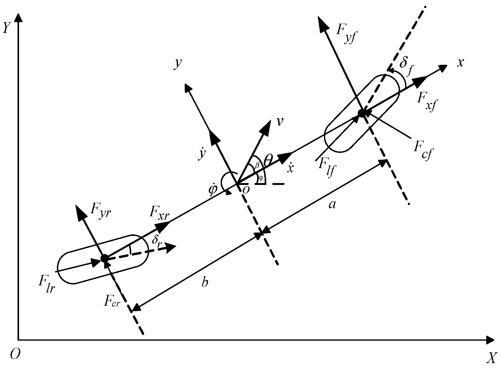
The three-degrees-of-freedom vehicle dynamics model was used as the predictive model for the predictive controller in this work. Figure 1 displays the vehicle’s three-degrees-of-freedom monorail dynamics model.
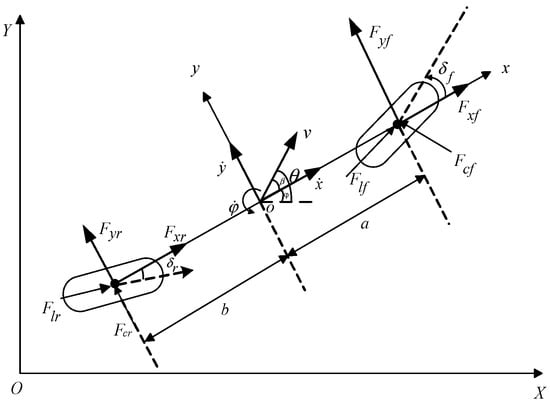
Figure 1.
Vehicle three-degrees-of-freedom monorail model.
The ferry vehicle’s degree of freedom in the transverse, longitudinal, and swinging directions is represented by the three-degrees-of-freedom model, which corresponds to the -axis, -axis, and -axis of the vehicle coordinate system. Therefore, the equilibrium equations of forces in the -axis, -axis, and -axis are established according to Newton’s second law.
where and are the driverless ferry vehicle’s accelerations along the and directions, respectively; is the vehicle’s total mass; is the heading angle acceleration; is the moment of inertia of the driverless ferry vehicle around the z-axis; and are the longitudinal force on the front and rear wheels of the driverless ferry vehicle in the x-axis direction; and are the lateral forces on the front and rear wheels of the driverless ferry vehicle in the -axis direction, respectively; is the speed of the driverless ferry vehicle along the -axis; is the heading angular speed of the ferry vehicle; and distances and , respectively, are measured from the driverless ferry vehicle’s center of mass to its front and rear axles.
The longitudinal and lateral forces acting on the tires can indicate parameters such as slip rate, road friction coefficient, tire slip angle, and the vertical load of the ferry vehicle.
where is the tire’s slip angle, is the slip rate, is the road friction coefficient, and is the vertical load on the driverless ferry vehicle tire.
The following conversion equation is obtained by converting the body coordinate system to the inertial coordinate system:
By combining Formulas (6) and (7), the vehicle’s nonlinear dynamic model can be established. The road friction coefficient, , can be obtained under the given road conditions. Finally, the system is described using a state space expression, as shown below:
The state variable in this system is configured as . The driverless ferry vehicle has front-wheel steering. Hence, the rear-wheel steering angle is . As a result, is used as the control variable, while is chosen as the output quantity. In the model predictive controller covered in the study, this model acts as the predictive model.
3. Longitudinal Controller Design
Figure 2 displays the schematic diagram for the longitudinal motion control. It mainly includes acceleration/brake mode switching logic, fuzzy PID controller, and brake controller. The acceleration/braking mode switching logic judges the driving/braking state of the vehicle according to the expected acceleration obtained by the upper controller, and it realizes the switching between acceleration and deceleration by adding the switching logic of the acceleration tolerance interval to avoid frequent acceleration and deceleration switching, which affects the comfort and stability of speed control. The fuzzy PID controller calculates the expected acceleration according to the deviation between the expected speed and the actual feedback speed, adaptively adjusts the PID control parameters through the established fuzzy rule table, and finally inputs the motor torque. The brake controller is converted into the brake oil pressure according to the difference between the expected speed and the actual speed. The longitudinal motion controller designed in this section considers only the deviation from the expected speed and does not consider the influence of lateral motion for the time being.
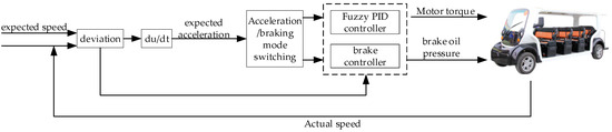
Figure 2.
Longitudinal motion control schematic.
3.1. Fuzzy PID Acceleration Controller Design
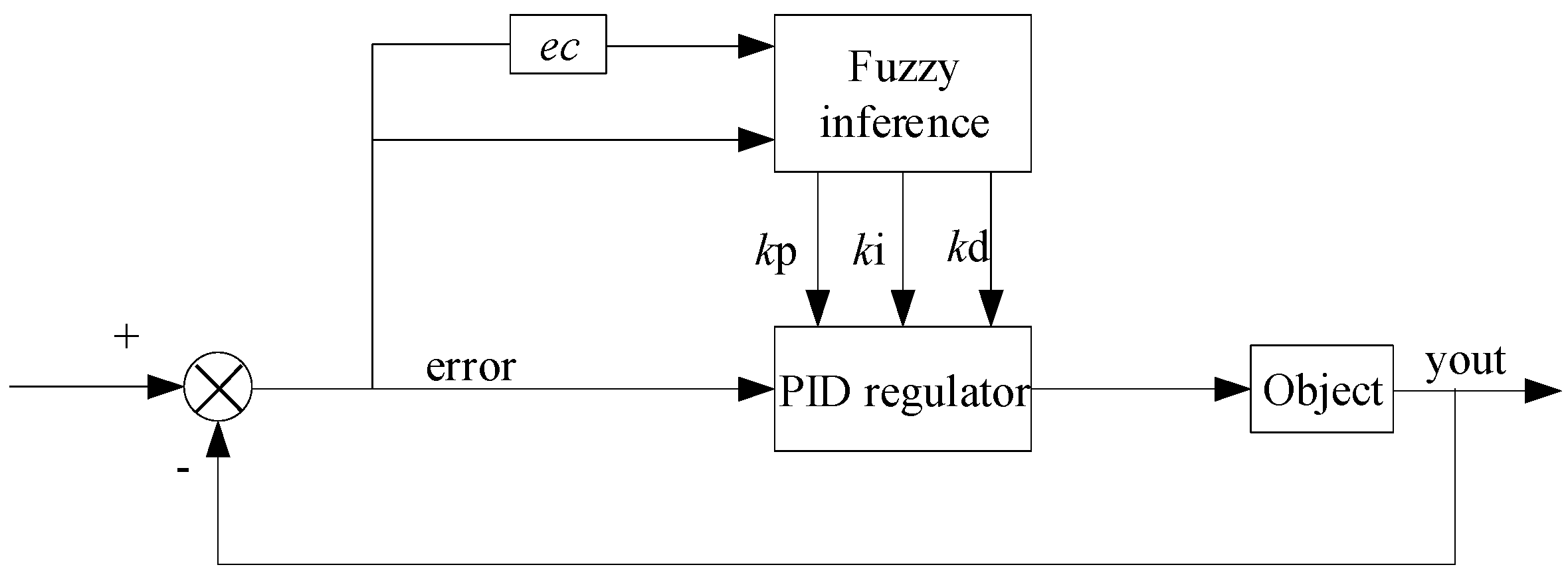
The fuzzy PID acceleration controller designed in this article uses a combination of fuzzy control [16] and PID control to realize the real-time online adjustment of PID parameters, thereby realizing the adjustment of the motor torque of the ferry vehicle, so as to achieve the real-time speed regulation of the vehicle. Figure 3 shows the fuzzy PID controller’s structure diagram.
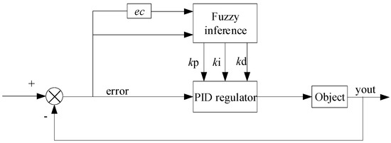
Figure 3.
Fuzzy PID controller’s structure diagram.
3.1.1. Controller Structure
A two-dimensional fuzzy controller [17] was chosen for this paper; that is, the speed deviation () and the variation () of the speed deviation are taken as double inputs, and the expected acceleration of the ferry vehicle () is taken as the single output control quantity. The changes in velocity deviation and velocity deviation are shown in Formulas (9) and (10), respectively.
where represents the ferry vehicle’s actual speed, and is its intended speed.
3.1.2. Fuzzification
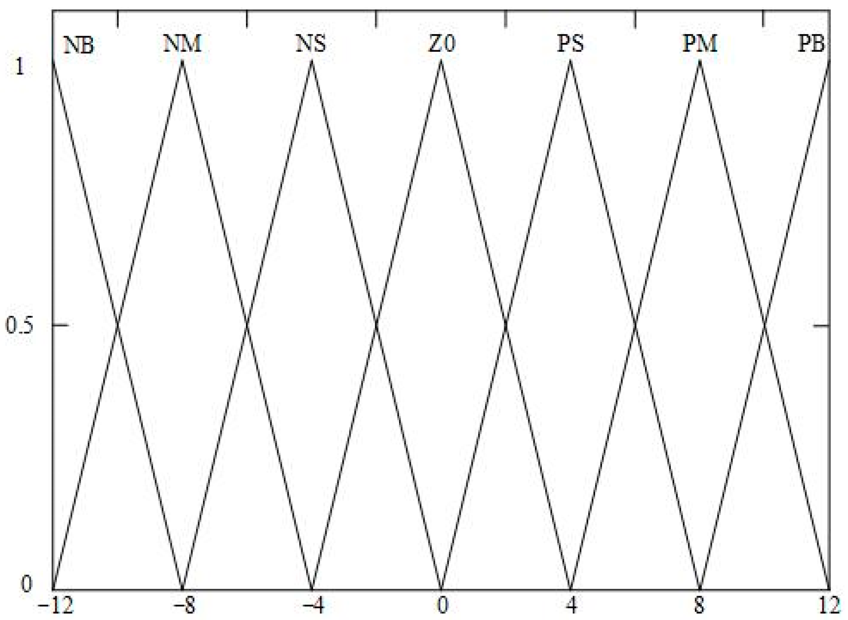
The steepness of the membership function curve affects the control performance. The higher the steepness, the higher the resolution and the faster the response speed; the lower the steepness, the lower the resolution and the slower the response speed. When the driverless vehicle is in motion, its control response should be faster, so this paper uses the triangle membership function as the membership function in fuzzification [18], the following is the triangular membership function:
In the formula, .
The range of the speed deviation () and the speed deviation change rate () in the fuzzy controller are both defined as [−12, 12], so the domain of the speed deviation () and the speed deviation change rate () are both [−12, 12]. The output of the fuzzy controller is , , and , as shown in the following equation:
where , , and are the PID controller’s starting parameters; and , , and are the fuzzy controller’s online adjustment parameters.
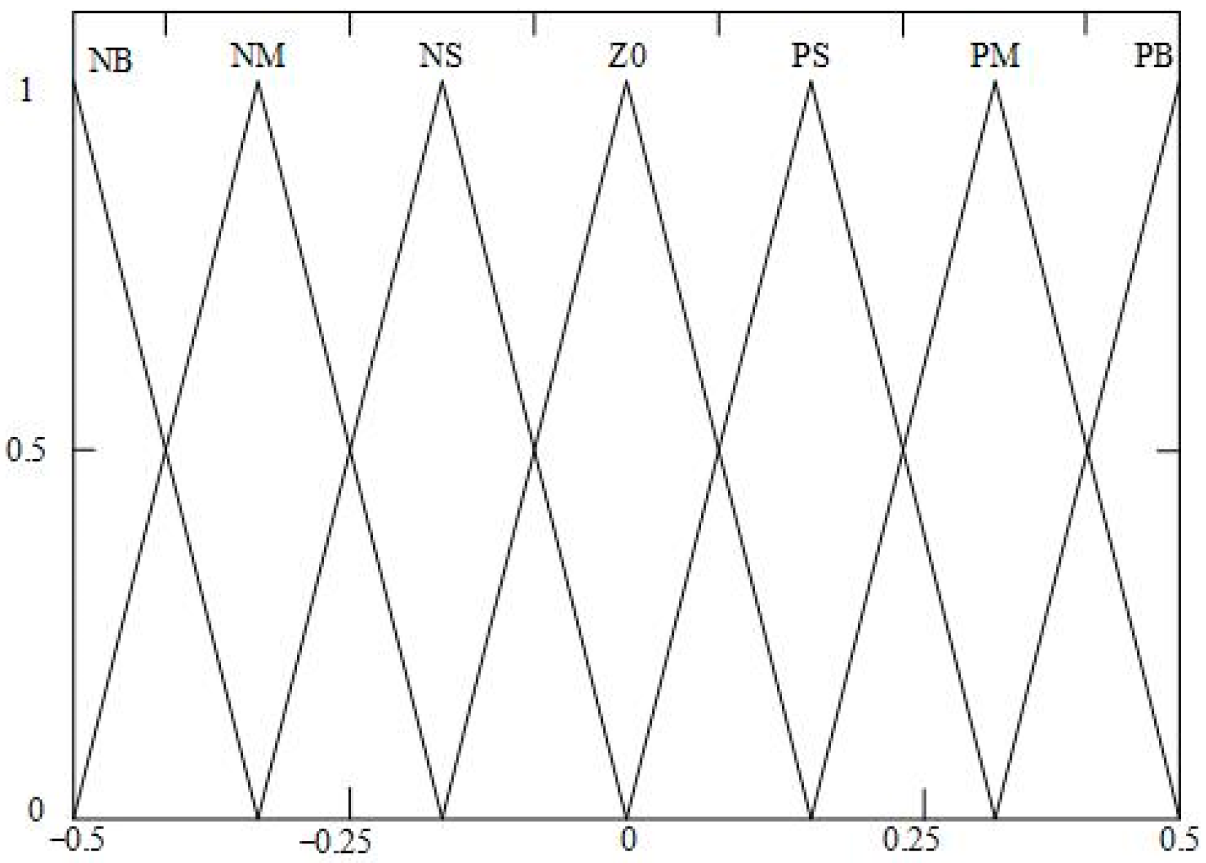
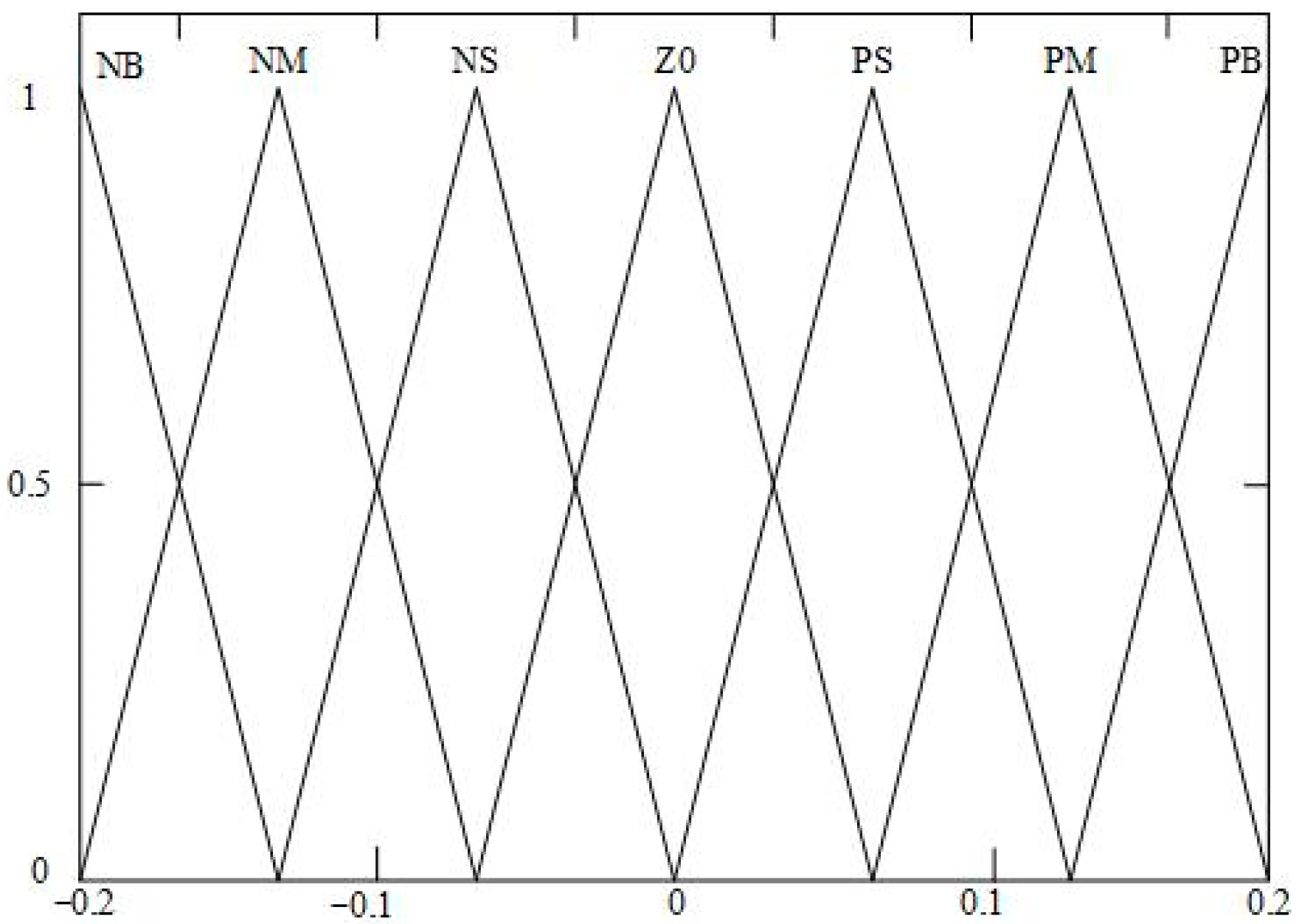
The fuzzy domain of is defined as [−0.5, 0.5], and the fuzzy domain of and is defined as [−0.2, 0.2]. Figure 4, Figure 5 and Figure 6 display the fuzzy controller’s input and output variable affiliation functions, respectively.

Figure 4.
Membership function of and .
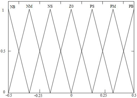
Figure 5.
Membership function of .
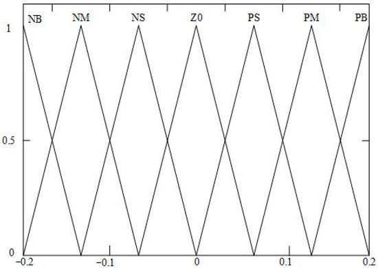
Figure 6.
Membership function of and .
3.1.3. Fuzzy Rules
The values of , , and are adjusted online in real time by fuzzy rules. According to the expert experience, the fuzzy set is defined as {negative big, negative middle, negative small, zero, positive small, median, positive big} seven grades; that is, the fuzzy set is . Therefore, the selection of fuzzy rules is based on the following: When the speed deviation and the speed deviation change rate are large, in order to quickly reduce the system deviation, a larger and and a smaller should be selected. When the rate of change of velocity deviation and velocity deviation is small but there is an obvious oscillation phenomenon, so as to quickly decrease the oscillation phenomenon and restore the stability of the system, a smaller and and a larger should be selected. When both the velocity deviation and rate of change of velocity deviation are less than or equal to 0, the ferry is in deceleration or uniform motion, and the acceleration control should not work, so , , and should be 0. The specific fuzzy rules are shown in Table 1.

Table 1.
Fuzzy rule table.
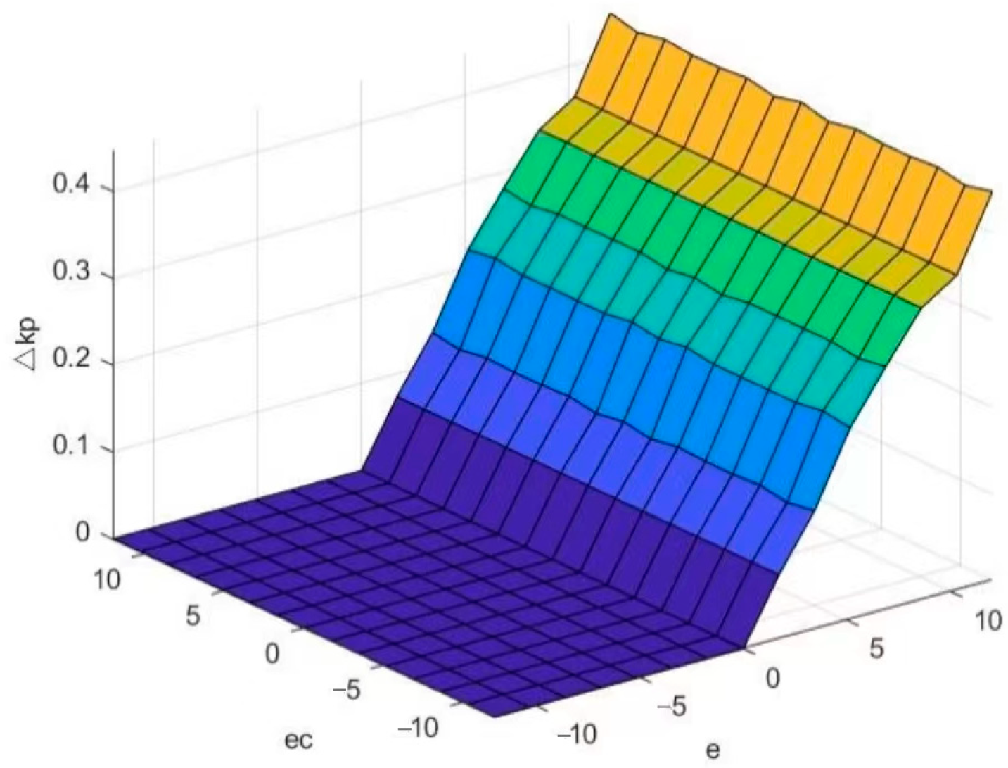
By compiling the domain of each parameter and the defined fuzzy rules into the fuzzy control toolbox of MATLAB, the relationship between the parameters can be observed clearly, such as the fuzzy rule surface diagram of the corresponding relationship between the parameters, as shown in Figure 7, Figure 8 and Figure 9.

Figure 7.
Fuzzy regular surfaces of .
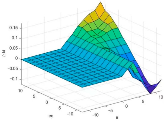
Figure 8.
Fuzzy regular surfaces of .
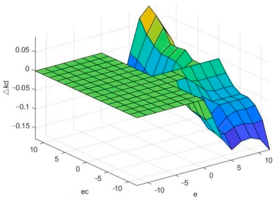
Figure 9.
Fuzzy regular surfaces of .
The final designed fuzzy PID acceleration controller finally outputs the motor torque of the vehicle, and the design flow is shown in Figure 10:
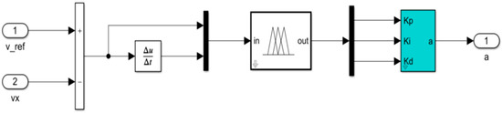
Figure 10.
Fuzzy PID acceleration controller.
3.2. Brake Control Design
To complete the braking control of the driverless ferry vehicle in the driverless state, the braking torque is calculated using the difference between the desired speed and the current speed. Consequently, the braking oil pressure is an output based on the relationship between the braking torque and the braking oil pressure. The braking control schematic diagram is shown in Figure 11.
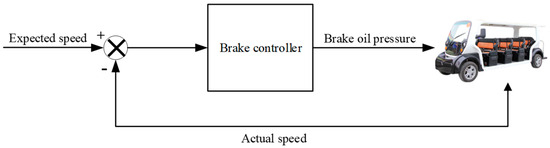
Figure 11.
Brake control principle.
The driverless ferry vehicle’s required braking deceleration is computed based on the difference between its desired and actual speeds. The braking deceleration formula is as follows:
In Formula (13), the driverless ferry vehicle’s braking deceleration is represented by , its desired speed is represented by , its actual speed is represented by , and its braking duration is represented by .
According to Newton’s second law, the braking force needed for the driverless ferry is calculated. It contains an equal distribution of the entire braking force across the four wheels. The following is the formula for calculating the braking torque of each wheel:
In Formula (14), is the braking torque required by a single wheel, and is the wheel radius.
The relationship between torque, force, and force area determines how the braking torque is converted to brake oil pressure. The relationship equation is as follows:
where represents the braking force exerted by the brake calipers, represents the effective friction radius of the brake disc, represents the caliper piston area, and represents the brake oil pressure.
3.3. Acceleration and Braking Mode Switching Controller
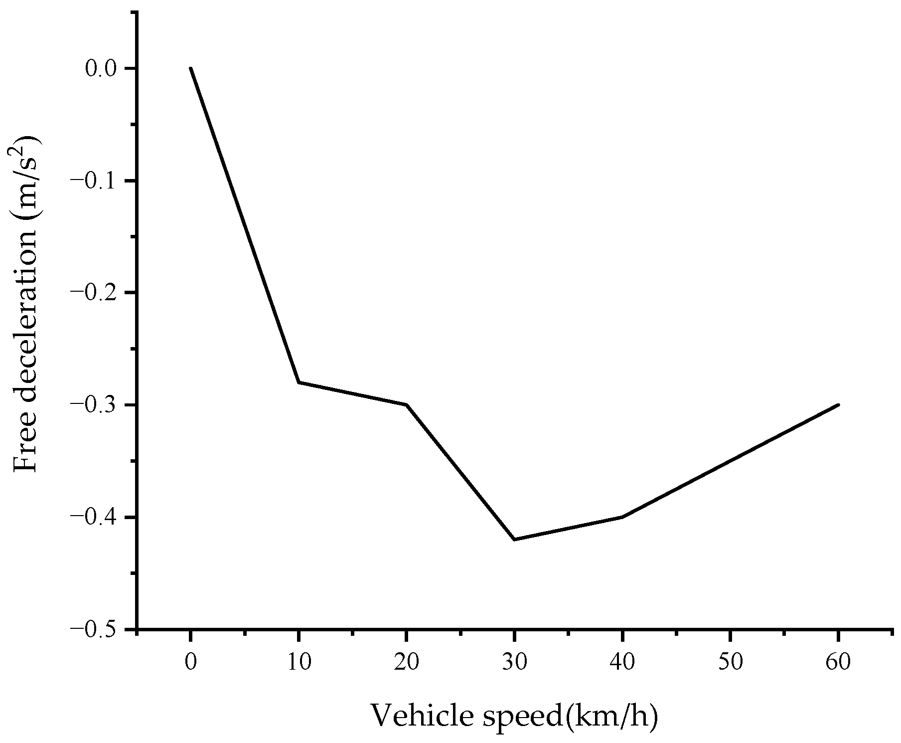
A tolerance zone is added to the design of the longitudinal controller to make the ferry vehicle slowly accelerate and brake so as to prevent the frequent switching of acceleration control and braking control, which impacts the comfort and stability of speed control. When the ferry vehicle releases the acceleration pedal and the brake pedal, it stops under the action of all kinds of resistance, calculates the maximum free deceleration of the ferry vehicle, and obtains the relationship between the deceleration and the speed of the ferry vehicle. The deceleration formula of the ferry vehicle is as follows:
In Formula (17), is the free deceleration, is the desired speed, and is the time taken by the ferry vehicle from the expected speed to the stop.
The testing of the vehicles was achieved by employing different speeds and using experimental methods, and the relationship between the free deceleration of the ferry vehicle and the speed is shown in Figure 12.

Figure 12.
Relationship between vehicle speed and maximum free deceleration.
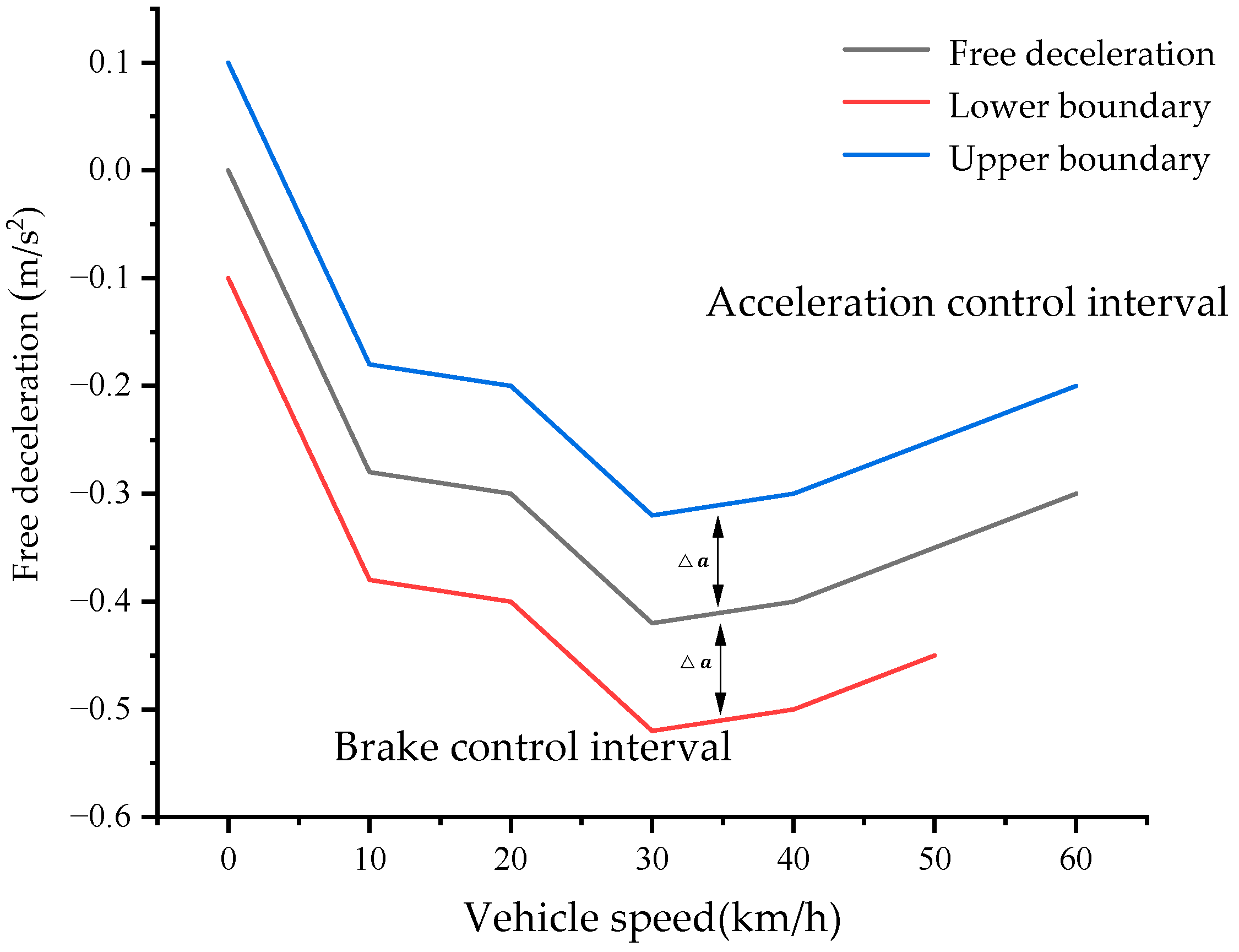
According to the actual vehicle debugging and experience, the acceleration tolerance interval is taken as , and the acceleration and braking switching rules are established through the expected acceleration () and the maximum free deceleration () as follows:
At , the driverless ferry vehicle has reached the upper boundary of the tolerance interval and is in the acceleration control interval, so it is necessary to control the acceleration of the vehicle and then input it into the fuzzy PID controller according to the calculated ; thus, calculate the required motor torque, and the braking control does not work at this time.
At , the driverless ferry vehicle has reached the tolerance range, and the vehicle does not do anything in the tolerance zone; that is, it does not accelerate or brake, keeping the original state of the vehicle.
When , the driverless ferry vehicle reaches below the lower boundary of the tolerance interval and is in the braking control interval, it is necessary to brake the vehicle and then convert the brake oil pressure needed by the vehicle according to the difference between the expected speed and the actual speed, and the acceleration control does not work at this time.
The curve of the switching rule of acceleration and braking is shown in Figure 13.
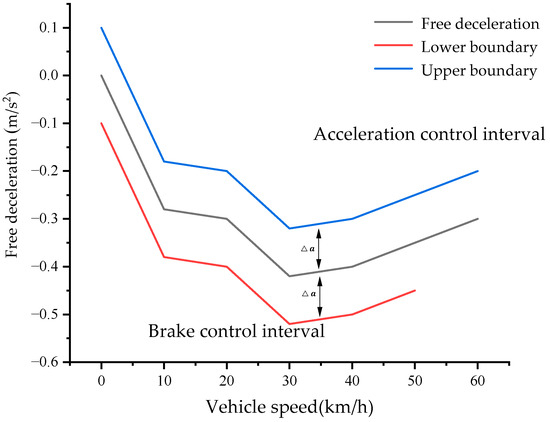
Figure 13.
Acceleration/braking switching rule curve.
4. Obstacle Avoidance Algorithm and Transverse Controller Design
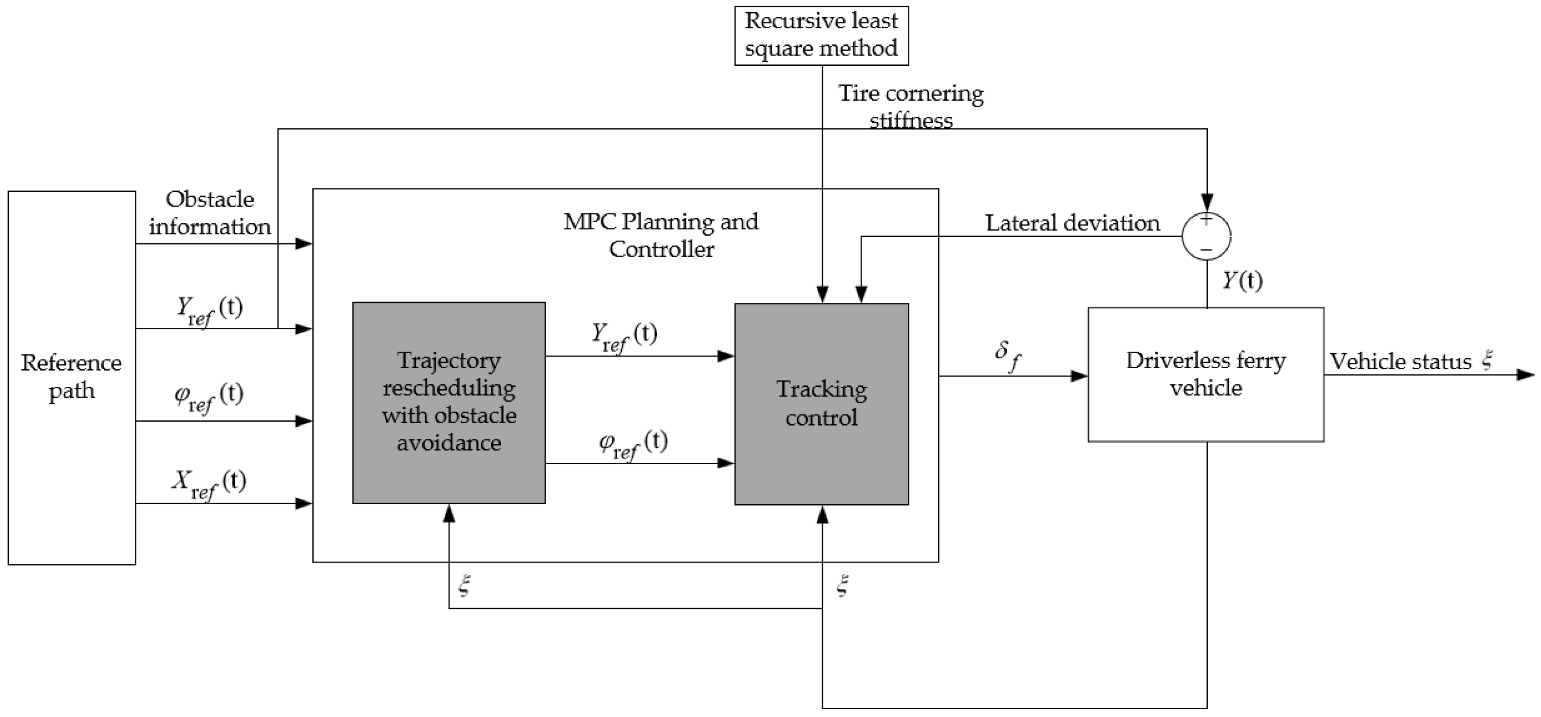
Figure 14 is a schematic diagram of lateral motion control. The trajectory planning and tracking controller receive the reference path information, the vehicle state information, and the estimated tire cornering stiffness. Through the trajectory rescheduling module and the MPC tracking control module, the front-wheel angle is finally output to the actuator of the ferry vehicle, and the lateral motion control of the driverless ferry vehicle is finally realized.
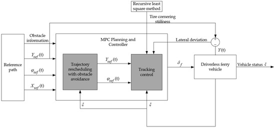
Figure 14.
Schematic diagram of lateral motion control.
4.1. Analysis of Tire Cornering Stiffness
In this paper, the tire lateral deflection stiffness of a driverless ferry vehicle is estimated by the recursive least squares method [19]. The linear regression equation between tire cornering force and tire linear cornering stiffness is as follows:
where is the regression vector, and is the model parameter to be estimated.
The goal of recursive least squares-based model parameter estimation is to minimize the squared difference between the estimated and actual values inside the study window of historical data. This difference can be represented as the cost function, :
in the formula, is the forgetting factor, is the length of the time window, and is the estimated value of model parameters.
After deducing, the recursive formula for recursive least squares can be obtained as follows:
Recursive gain:
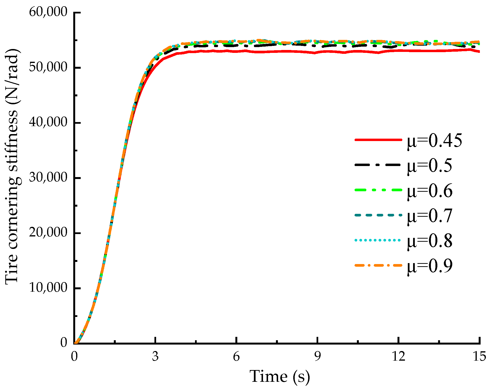
The tire lateral deflection stiffness estimation model was built in MATLAB/Simulink, the recursive least squares algorithm was compiled in the S-Function module, and the joint simulation with CarSim 2019.0 software was carried out to solve the estimated tire cornering stiffness. Figure 15 shows the tire side stiffness results estimated under different road adhesion coefficients.
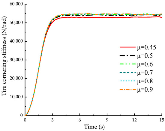
Figure 15.
Estimation results of tire cornering stiffness under different road adhesion coefficients.
4.2. Design of MPC Controller with Planning Module
4.2.1. Trajectory Planning Layer Design
In this study, a new trajectory planning and tracking controller was obtained by adding a planning module to the MPC trajectory tracking controller. The added trajectory planning layer meets the following three conditions:
- (1)
- The deviation between the desired trajectory of the vehicle obtained by the planning module and the reference trajectory obtained by the global planning should be as small as possible.
- (2)
- The expected trajectory obtained by the planning module should meet the dynamic constraints of the ferry vehicle.
- (3)
- The added trajectory planning module should be able to avoid obstacles.
The most important content in the trajectory planning module is the trajectory replanning algorithm. The main function of the trajectory replanning algorithm is to design a reasonable evaluation function, which can realize the obstacle avoidance function of the driverless ferry vehicle when the evaluation function satisfies various constraint conditions. And, in the whole tracking control process, the deviation between the driverless ferry and the global reference trajectory is as small as possible.
(1) Obstacle avoidance function
The obstacle avoidance function used for the thesis modifies the function value’s magnitude based on the variation in the distance between the obstacle point and the ferry vehicle. Specifically, as the distance increases, the function value decreases; conversely, as the distance decreases, the function value increases. The following formula is the obstacle avoidance function:
where is the weight coefficient; ; in the vehicle coordinate system, the obstacle point’s coordinate is ; is the vehicle centroid coordinate; and is a little positive number that prevents the denominator from being 0.
By adjusting the weight coefficient in the formula to make the ferry avoid obstacles, The greater the weighting coefficient’s value, the more conservative the results behave, which will cause the planned path to avoid obstacles. When there are no obstacles on the road, the function will not have any impact on the planning [20].
(2) Point-mass model
Considering the control effect of the algorithm and the calculation speed, the planning module uses a point-mass model that treats the entire vehicle as a point with mass. [21]. For the mass vehicle dynamics model of the driverless ferry vehicle point, the resultant transverse and longitudinal forces of the ferry tire should satisfy the constraint of the friction circle.
where is the proportionality factor, and , limiting the tire friction saturation. The vehicle point mass model is as follows:
After considering the dynamic constraints of the vehicle, the constraints are added, as shown below:
Finally, the point mass model can be simplified as follows:
In the formula, , and there are a total of five state variables, namely the speed of the ferry vehicle on the and axes, the heading angle of the ferry vehicle, the longitudinal position of the ferry vehicle, and the lateral position of the ferry vehicle. In addition, is the control quantity.
(3) Curve fitting
In the trajectory replanning algorithm, the trajectory planned by the planning module is given in the form of predicting discrete points in the time domain, and the discrete points are fitted with a quintic polynomial curve [22,23]. The formula for the quintic polynomial is as follows:
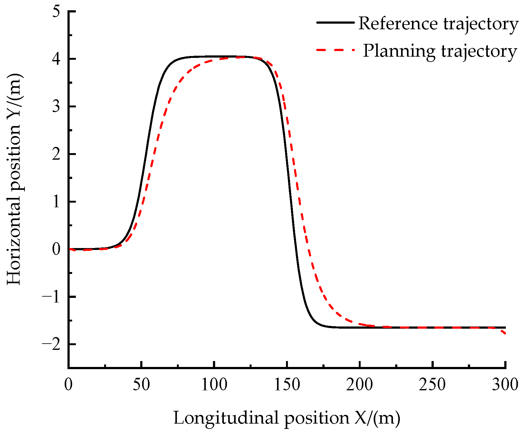
In the formula, and are the parameters to be obtained. Considering that the road has both straight lines and bends, the double shift line condition is selected as the road to verify the algorithm in this paper. The reprogrammed trajectory of the reference trajectory with a fifth-degree polynomial fit is shown in Figure 16.

Figure 16.
Reference trajectories and planning trajectory.
In Figure 16, the obstacle appears at 50 m, it can be seen that the obstacle avoidance function can avoid the obstacle better, and the quintic polynomial can fit the replanning trajectory better. It is proved that the obstacle avoidance function selected in this paper and the quintic polynomial curve fitting method are effective.
4.2.2. Tracking Control Layer Design
Because the controlled object is a driverless ferry car, which is a complex nonlinear system. Firstly, the nonlinear model is linearly discretized [24], then the constraint conditions and objective function are designed, and finally, the angle of the front wheel is resolved, as shown in Figure 17, which is the trajectory-tracking flowchart.
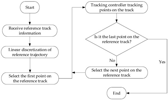
Figure 17.
Trajectory-tracking flowchart.
4.2.3. Linear Discretization of Nonlinear Models
Here we discuss the linearization of a ferry vehicle’s nonlinear dynamics model using a linearization method for state trajectories.
Let be the state quantity and control quantity at a certain time in the system, and let represent the system state quantity obtained when the system continuously outputs the control quantity, The following relationships exist between them:
The system of Equation (31) is transformed into a linear time-varying system equation:
where , , , .
The discretization of the above formula can be obtained:
By combining Formula (32) with Formula (33), you can obtain the following:
where , and .
According to the above linear discretization method, the nonlinear dynamic equation of the driverless ferry vehicle is linearized, and the linearized equation is obtained as follows:
in the formula , .
Among them, , , and .
Discrete state-space expressions are created by discretizing the linearized equations derived previously using the first-order difference quotient method:
where is .
4.2.4. Establish Constraints
When establishing the constraint conditions, the vehicle dynamics limitations should be taken into account in addition to the control quantity and control increment constraints.
(1) Control quantity and control increment constraints
Based on real vehicle testing, it was found that the front wheel of the ferry vehicle turns left to the limit position and from the center position to the right to the limit position is 20 degrees, so that the rotation angle of the wheel to the left is negative; otherwise, it is positive [25]. Therefore, the constraint condition is set to the following:
(2) Centroid lateral deflection angle constraint
Since the road surface driven by the ferry vehicle in the school is a smooth asphalt pavement, it is only necessary to consider that the centroid side slip angle is kept within a reasonable range when the ferry vehicle is driving on a good road surface, and the constraint condition of the centroid side slip angle is as follows [26]:
(3) Tire slip angle constraint
At t time, the tire slip angle can be expressed as follows when the system’s state variables are known:
According to the tire cornering properties, at tire side deflection angles less than 5 degrees, the tire’s side deflection angle is directly proportional to the side deflection force [27], and the following is the restriction condition for the tire slip angle:
4.2.5. Objective-Function Design
In the solution, the goal function, which is as follows, must be used to determine how to optimize the system state quantity and control quantity.
where represents the actual output; represents the reference output; is the predictive time domain; is the control time domain; is the weight coefficient; and is the relaxation factor, which is used to avoid the collapse of the control system.
The derivation process for the future output of the linear error model of the driverless ferry vehicle is as follows:
Convert Formula (34) into the following form:
The following is the new state-space expression that is obtained:
where , , , .
After deducing as above, the system’s forecast output expression looks like this:
In the formula, , , , and .
By adjusting the objective function to a quadratic function model, the following can be obtained:
In the formula, , , and .
The following control input increments are obtained by solving the aforementioned equation for each control cycle:
The control system applies the first control input increment as the real control input increment for the system in the manner described below:
Before the next time comes, the control system will continue to execute the control quantity, and after entering the next sampling time, repeat the above process until the whole system completes the control process.
4.3. Coordinated Control Design
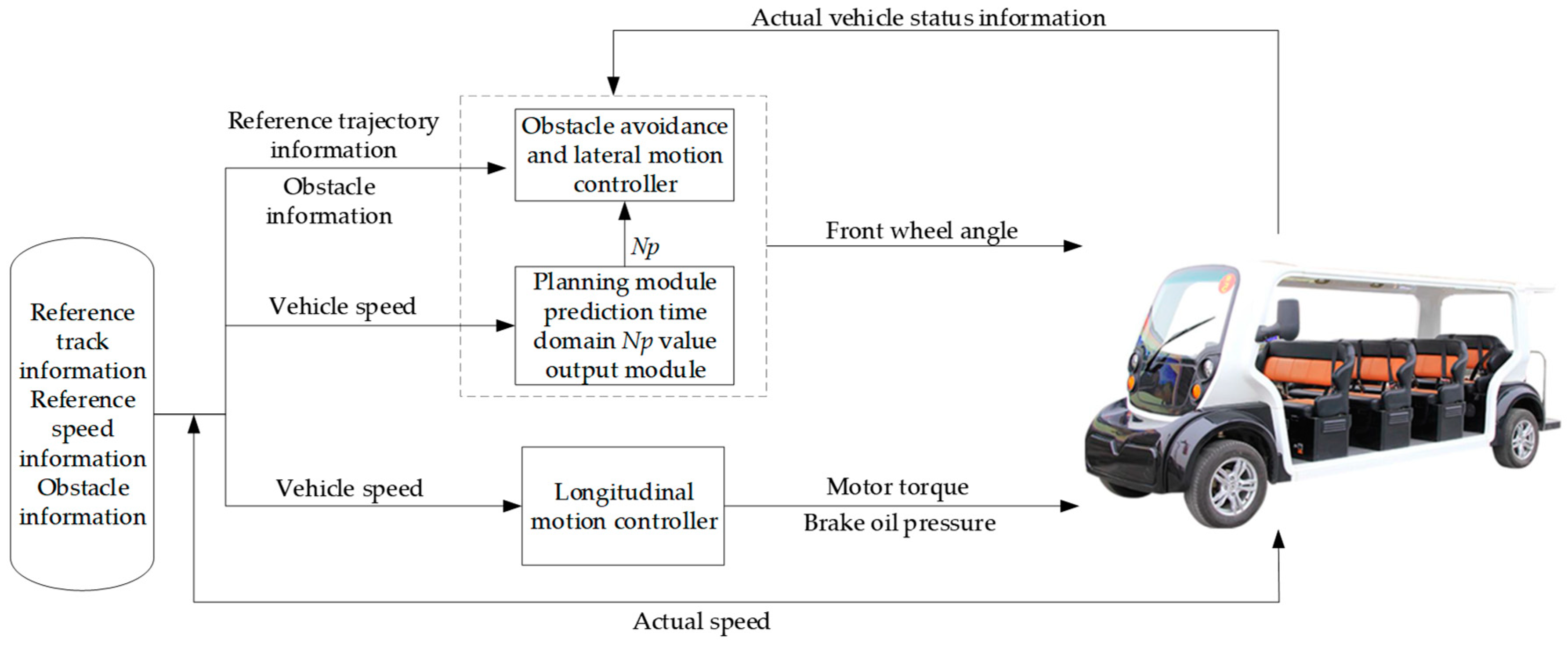
The results of the lateral simulation in Section 4.2 show that different speeds correspond to different parameters of the lateral motion controller, the vehicle speed is an important input of the longitudinal motion controller, and the impact of avoiding obstacles When the speed is below 18 km/h and the matching predictive time domain is 7, replanning works well. When the vehicle speed is greater than 18 km/h and less than 36 km/h, the corresponding prediction time domain is 10, and the effect of obstacle avoidance replanning is the best. Therefore, the primary vehicle speed information is used to coordinate and regulate the driverless ferry vehicle’s horizontal and longitudinal motion. The speed-planning module is designed to predict the two-dimensional time-domain look-up table module, and the optimal predicted time-domain values of different speeds and their corresponding are input into the two-dimensional look-up table module as a horizontal and vertical correlation module. When the vehicle speed is lower than 18 km/h, the corresponding prediction time domain is 7, and when the speed is greater than 18 km/h less than 36 km/h, the corresponding prediction time domain is 10. Figure 18 illustrates the coordinated control structure that is both horizontal and vertical.
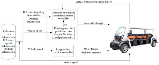
Figure 18.
Horizontal and vertical coordinated control structure diagram.
5. Simulation Analysis
Co-simulation was carried out by MATLAB/Simulink and CarSim, and the simulation condition is a double-shifted line condition. Because the roads driven by driverless ferry vehicles in the school are all asphalt pavements, a review of the data shows that both dry and wet asphalt pavements contain a pavement adhesion coefficient of 0.8. Therefore, the pavement adhesion coefficient was selected to be 0.8. Firstly, the longitudinal tracking effect of the vehicle with or without tolerance space is compared and analyzed via simulation under the condition of a constant speed of 35 km/h. Secondly, the lateral control effect of the vehicle under different speeds and different predictive time domains is analyzed. Finally, when the driverless ferry vehicle faces the unknown obstacles suddenly appearing in the front or rear half of the road under coordinated control, the effect of obstacle avoidance and trajectory tracking, the change of front wheel angle, the tracking effect of yaw angle, and the tracking error are compared with those of driverless ferry vehicle under uncoordinated control to analyze the coordinated control effect. Table 2 shows the main vehicle parameters, Table 3 shows the planning module parameter settings, and Table 4 shows the tracking controller parameter settings.
Table 2.
Some design parameters of a driverless ferry vehicle.
Table 3.
Planning module parameter setting.
Table 4.
Tracking controller parameter setting.
Set the weight matrix of the tracking controller to .
5.1. Longitudinal Motion Simulation Condition
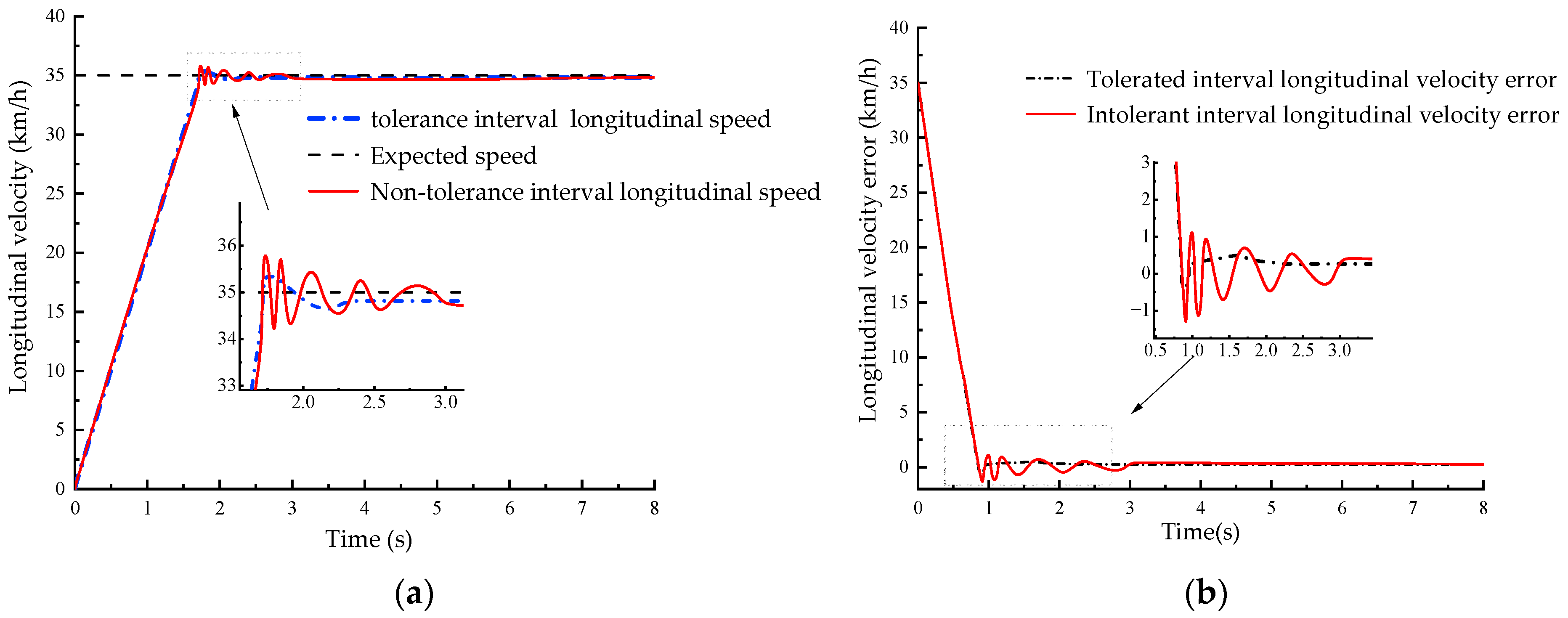
(1) Set the initial speed of the driverless ferry vehicle to 0, and the desired speed is constant at 35 km/h for the constant speed cruise simulation condition. The speed tracking of the driverless ferry vehicle is shown in Figure 19:
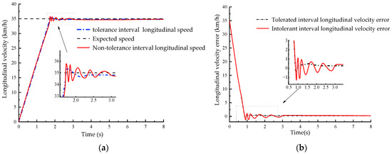
Figure 19.
Speed tracking and speed tracking error diagram when the expected speed is 35 km/h: (a) speed tracking effect and (b) speed tracking error.
As can be seen in Figure 19a, the longitudinal speed of the two longitudinal control strategies of the driverless ferry vehicle is compared in the process of trajectory tracking. In the case of longitudinal control without tolerance zones, although the ferry vehicle can finally stably track the desired trajectory, the longitudinal speed fluctuates greatly during the whole tracking process, resulting in the problem that the frequent switching between acceleration and braking modes of the ferry vehicle affects the comfort and stability of the speed control. When the longitudinal control with tolerance interval is adopted, the longitudinal speed fluctuation is significantly reduced, and the expected speed can be quickly tracked and stabilized, so that the driverless ferry vehicle accelerates in the braking mode, switching times are significantly reduced, and driving is smoother. As illustrated in Figure 19b, the longitudinal velocity error fluctuates greatly when there is no tolerance interval for longitudinal control, and the maximum longitudinal speed error is as high as 0.78 m. When the longitudinal control with tolerance interval is adopted, the maximum longitudinal speed error is about 0.44, the fluctuation of the longitudinal velocity error is significantly reduced, and the longitudinal velocity error tends to be stable faster, which is 43.59% lower than that of the intolerant interval. It can be seen that the stable speed and stability of the longitudinal motion controller designed in this study were significantly improved when tracking the expected speed, which effectively solves the problem that the driverless ferry vehicle switches between acceleration and braking modes too frequently, affecting the comfort and stability of speed control.
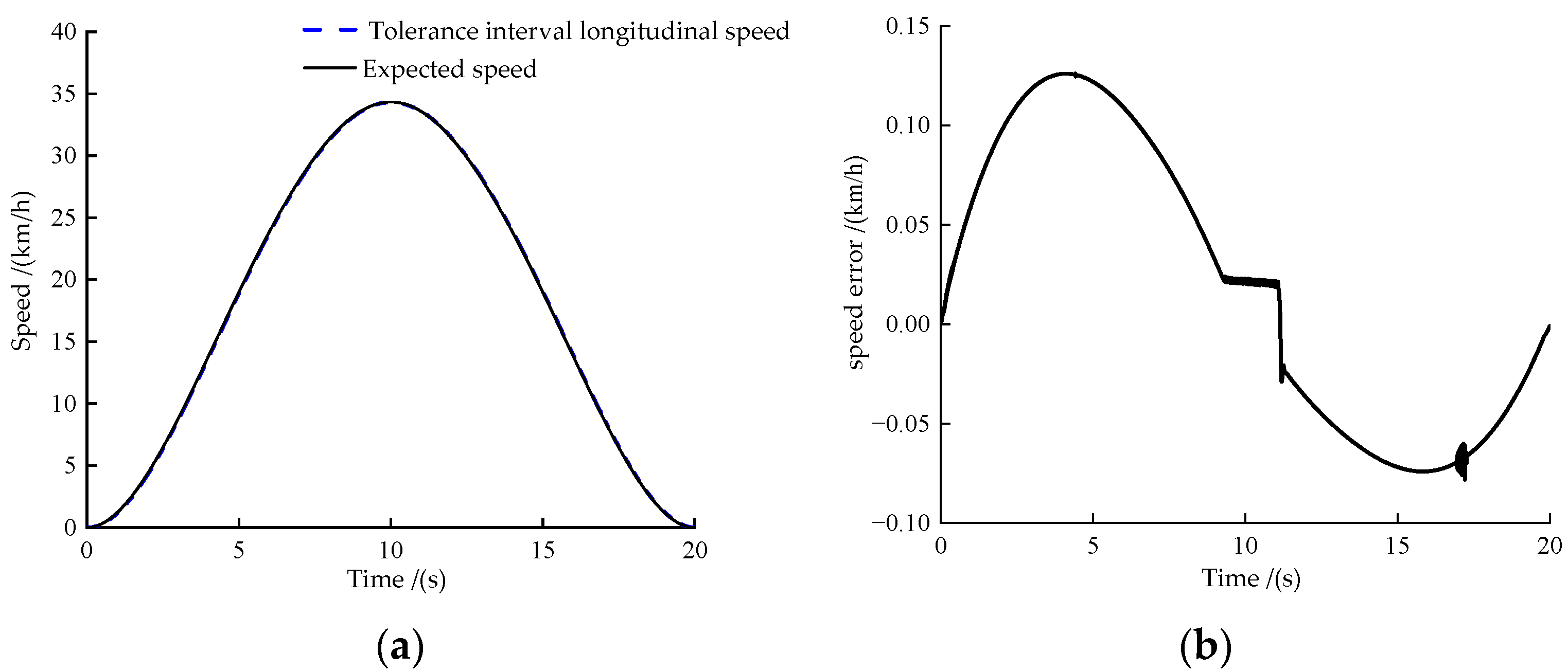
(2) Set the desired speed to a variable speed range from 0 to 35 km/h and then to 0, so that the ferry vehicle starts tracking when the initial speed is zero. The speed tracking of the driverless ferry vehicle is shown in Figure 20.
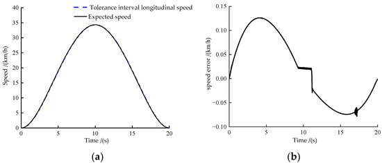
Figure 20.
Speed tracking and speed tracking error diagram when the expected speed is variable: (a) speed tracking effect and (b) speed tracking error.
As can be seen from Figure 20a, the driverless ferry can track the desired speed well during the whole speed tracking process. As can be seen in Figure 20b, at about 4 s after the start, the error in the whole tracking process is the largest, but it is also lower than 0.15 km/h, which fully meets the requirements of the vehicle, and the occurrence of such a situation at about 4 s may be due to the fact that the actuator of the vehicle has a delayed reaction when it is just running, and after the vehicle is running normally the effect of such a delayed reaction on the whole vehicle becomes very small. Generally speaking, the driverless ferry vehicle can still track the desired speed steadily and quickly when tracking with variable speed. It shows that the longitudinal motion controller designed in this paper still has a good tracking effect when tracking the variable speed, and it also makes a good prerequisite for the coordinated control of Section 3.3.
5.2. Lateral Motion Simulation Condition
The vehicle speed is 9 km/h, 18 km/h, and 36 km/h, respectively, and the prediction time domain () in the planning module is 7, 10, 15, and 20, respectively. The simulation comparison of the designed lateral motion controller for obstacle avoidance, replanning, and trajectory tracking was carried out, and the best value was selected. The simulation effects of the algorithm are shown in Figure 21, Figure 22 and Figure 23, respectively. Conditions 1, 2, and 3 are simulated at speeds of 9 km/h, 18 km/h, and 36 km/h, respectively, and with a road adhesion coefficient of 0.8.
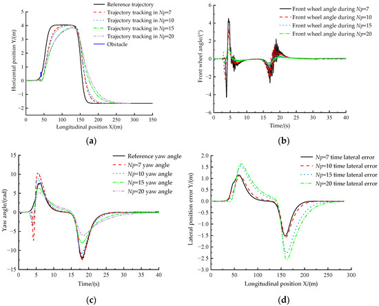
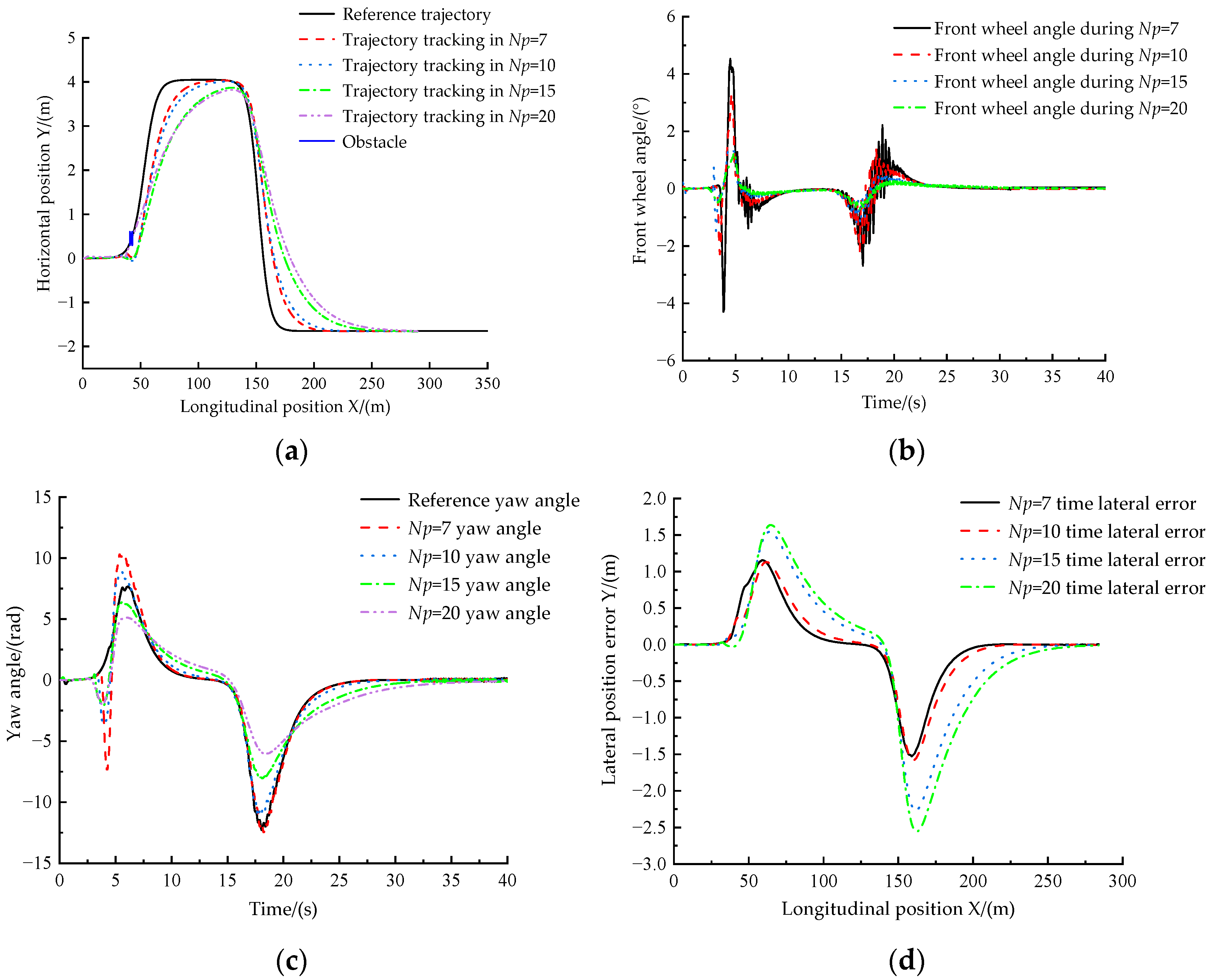
Figure 21.
Comparison of simulation results of control algorithms at 9 km/h: (a) obstacle avoidance replanning and trajectory tracking effect, (b) tracking effect of front wheel corner, (c) yaw angle tracking effect, and (d) lateral position error.
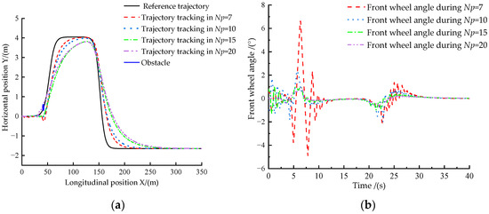

Figure 22.
Comparison of simulation results of control algorithms at 18 km/h: (a) obstacle avoidance replanning and trajectory tracking effect, (b) tracking effect of front wheel corner, (c) yaw angle tracking effect; and (d) lateral position error.
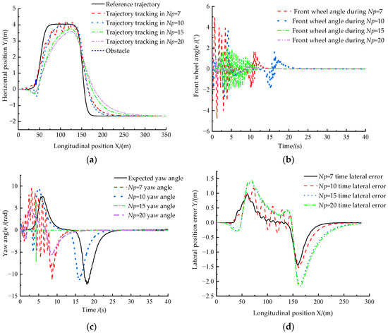
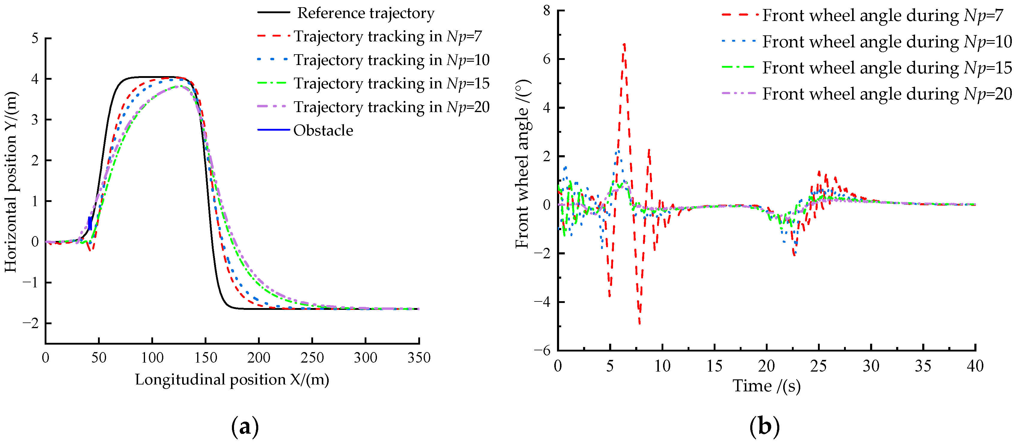
Figure 23.
Comparison of simulation results of control algorithms at 36 km/h: (a) obstacle avoidance replanning and trajectory tracking effect, (b) tracking effect of front wheel corner, (c) yaw angle tracking effect, and (d) lateral position error.
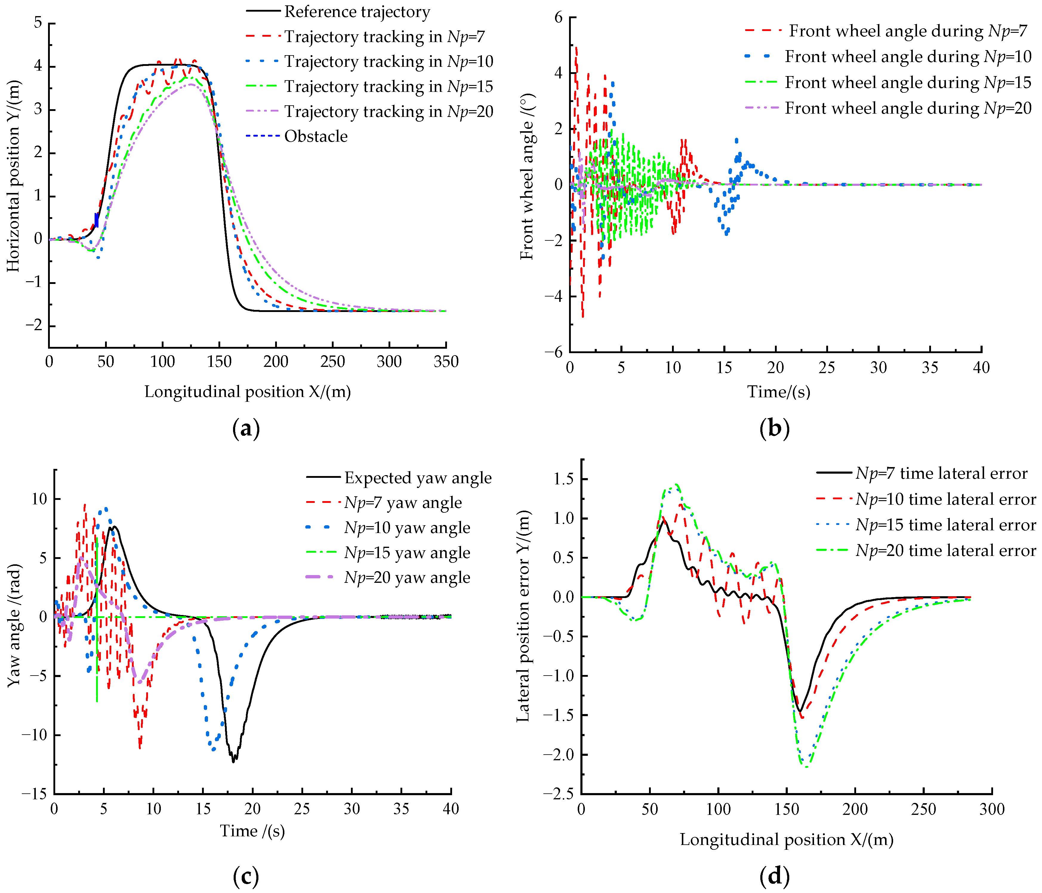
5.2.1. Condition 1
From Figure 21a, when the speed is 9 km/h, the passes through the obstacle; that is, it collides with the obstacle and tracks the reference trajectory poorly. The designed obstacle avoidance algorithm can better avoid obstacles and replan local trajectories when predicting time domain . Compared with other values, it has higher tracking accuracy. As seen in Figure 21b,c, the ferry vehicle encounters an obstacle at about 4 s and avoids it. In this local area, the actual yaw angle of the ferry vehicle no longer tracks the reference yaw angle, and the trajectory is replanned, which shows the rationality of the obstacle avoidance algorithm used in this paper. As seen in Figure 21d, the lateral position error of the driverless ferry vehicle at the obstacle avoidance and turning is larger, and the maximum error is as high as 2.7 m when . When , the maximum error is reduced to 1.5 m. Compared with other values, the tracking error of the driverless ferry vehicle is the smallest, and the tracking effect is the best. Therefore, when the speed is 9 km/h, the prediction time domain, , in the planning module is set to 7.
5.2.2. Condition 2
As seen in Figure 22a, when the speed is increased to 18 km/h, the autonomous ferry vehicle’s obstacle avoidance scenario is similar to that at a speed of 9 km/h, and the values can avoid obstacles smoothly, except for . As Figure 22b,c demonstrate, when the driverless ferry vehicle runs for about 4 s, it receives information about the obstacles ahead and avoids them, so the yaw angle of the ferry vehicle does not track the reference value. From Figure 22d, we can see that the maximum error still occurs at the turn, in which the tracking error of the driverless ferry vehicle is the smallest and the tracking effect is the best when predicting the time domain, . To sum up, when the speed of the driverless ferry vehicle is increased to 18 km/h, the predicted time domain, , value in the planning module is still set to 7.
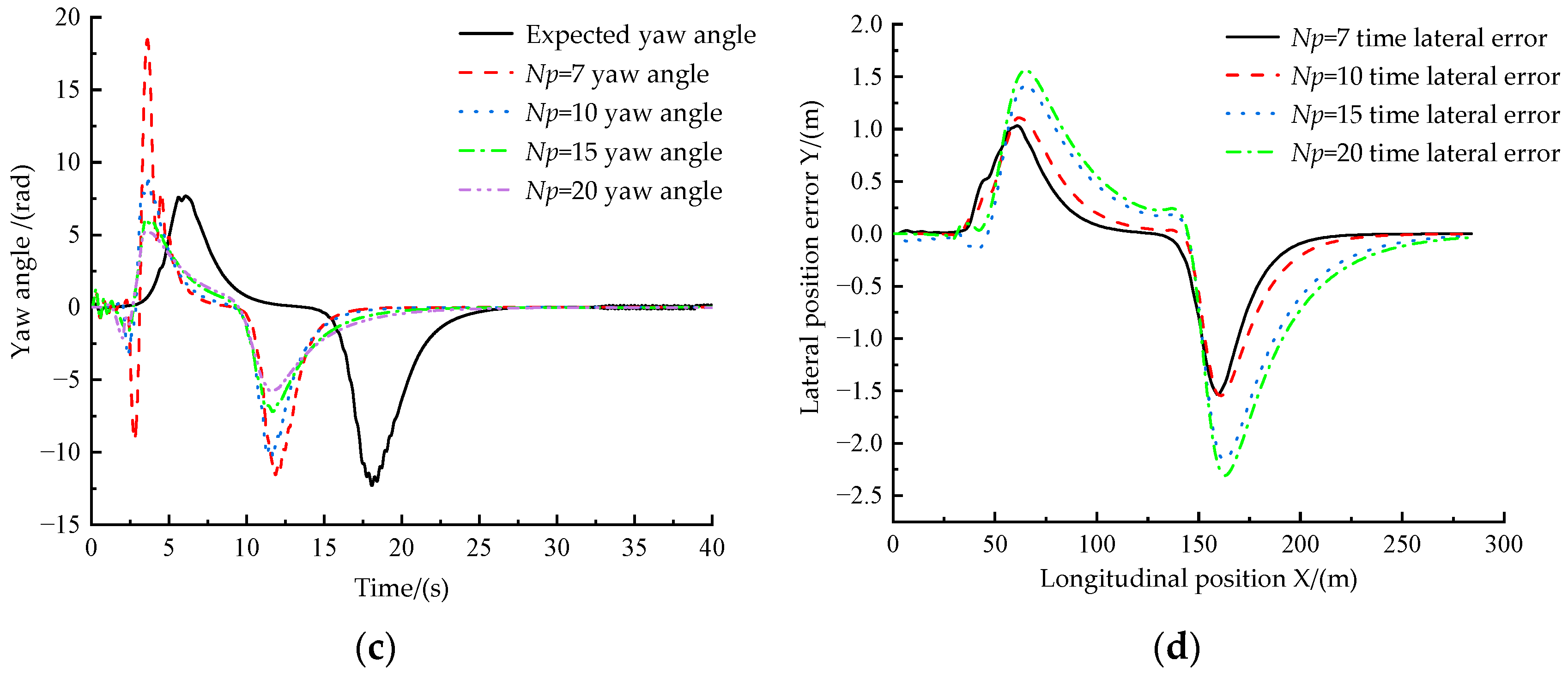
5.2.3. Condition 3
From Figure 23a, we can see that, when the speed is raised to 36 km/h, the designed obstacle avoidance function algorithm can avoid obstacles because of the high speed of the driverless ferry vehicle when the prediction time domain, , of the planning module is too high, while the other three cases can avoid obstacles smoothly. From Figure 23b,c, we can see that the tracking error of the driverless ferry vehicle to the expected yaw angle is minimum when . As can be seen from Figure 23d, except for , the tracking error of the driverless ferry vehicle is the smallest, and the tracking effect is the best when is used. Therefore, when the speed of the driverless ferry vehicle is increased to 36 km/h, the predicted time domain, , value in the planning module is set to 10.
To sum up, although the designed single-lateral motion controller with obstacle avoidance function has a certain ability for obstacle avoidance replanning and trajectory tracking, the tracking error is still more than 1 m when turning. It shows that the single-lateral motion control cannot enable the driverless ferry vehicle to track the reference trajectory stably. Therefore, on this basis, the coordinated control of horizontal and longitudinal motion should be designed.
5.3. Coordinated Control of Simulation Conditions
Conditions 1 and 2 are simulations with obstacles in the first half and second half of the roadway, respectively, and the roadway adhesion coefficients are both 0.8.
5.3.1. Condition 1
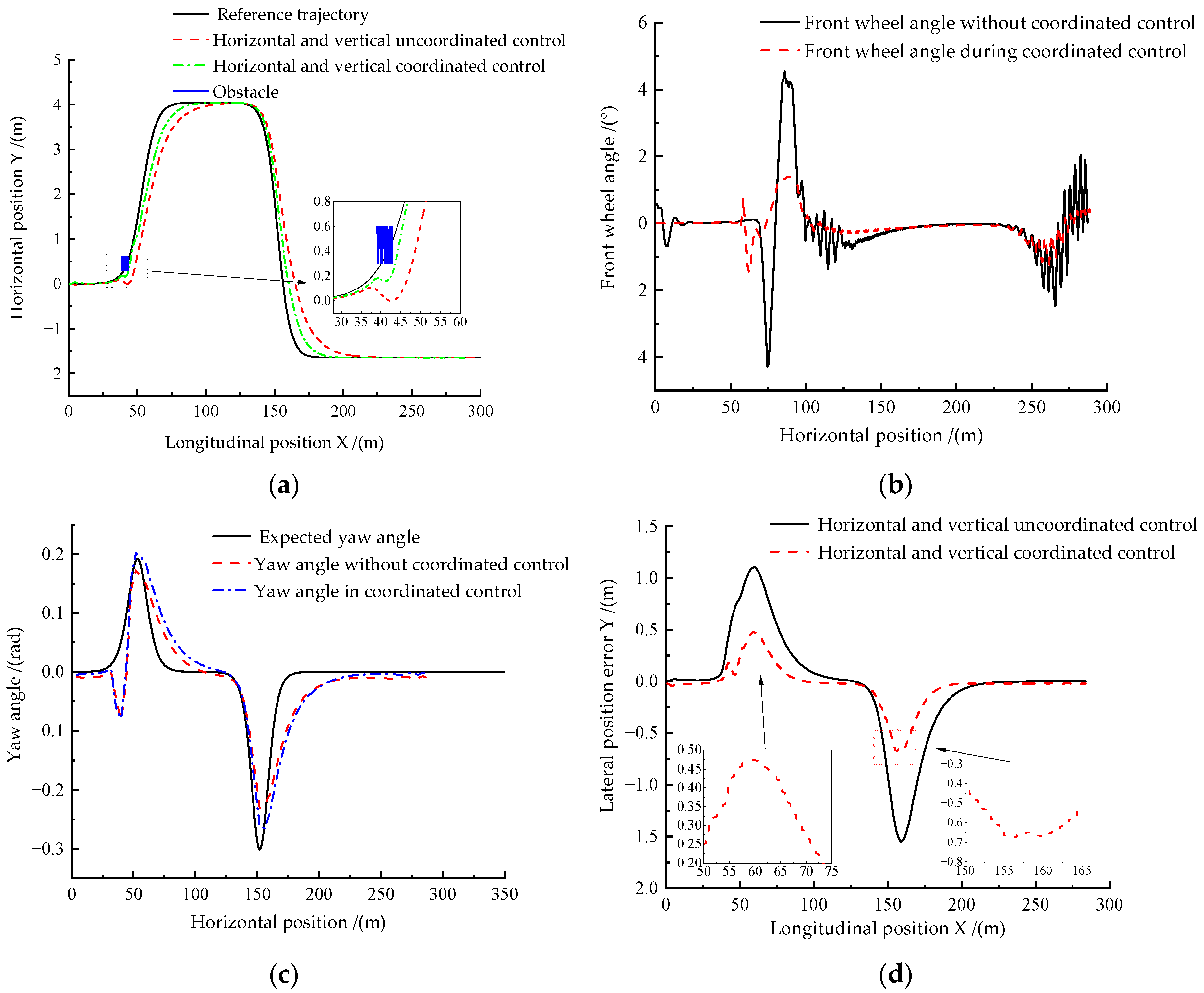
Under Condition 1, when unknown obstacles appear in the first half of the road, verification of obstacle avoidance replanning and trajectory tracking control of driverless ferry vehicles under double-shifted line conditions under coordinated control of horizontal and longitudinal controllers take place when the road adhesion coefficient is 0.8. Figure 24 illustrates the control algorithm’s simulation effect.
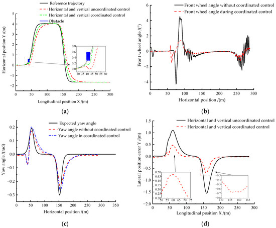
Figure 24.
Comparison of simulation results of control algorithms when obstacles are in front. (a) Comparison between obstacle avoidance replanning and trajectory tracking. (b) Comparison of front wheel angle. (c) Comparison of yaw angle tracking effect. (d) Comparison of lateral position error.
The horizontal motion and the longitudinal motion work separately; that is, there is no coordinated control. From Figure 24a, it can be seen that when the obstacle is in the first half of the path and there is no coordinated control in the horizontal and longitudinal directions, the driverless ferry vehicle is about to encounter obstacles and bends. Although it can avoid obstacles, the tracking accuracy of the reference trajectory is poor. When coordinated control is carried out horizontally and vertically, the tracking accuracy of the ferry vehicle relative to the reference trajectory is significantly improved. From Figure 24b,c, we can see that, when there is no coordinated control in the horizontal and longitudinal directions, the ferry vehicle will wobble frequently when it encounters obstacles. When horizontal and longitudinal coordinated control is carried out, the swing amplitude and frequency of the driverless ferry vehicle are greatly reduced, the output front wheel angle is more stable, and the tracking stability of the expected yaw angle is significantly improved. Figure 24d shows that, in the absence of coordinated control in the horizontal and vertical directions, the maximum lateral position error has exceeded 1.5 m. However, when coordinating control horizontally and vertically, the maximum horizontal position error is reduced to less than 0.7 m, and the tracking error is reduced by 53.33% compared to uncoordinated control in the horizontal and vertical directions. Through the above analysis, we can see that when there are obstacles in the front half of the road, the horizontal and longitudinal motion coordination control strategy designed shows a more outstanding effect of obstacle avoidance replanning and trajectory tracking control.
5.3.2. Condition 2
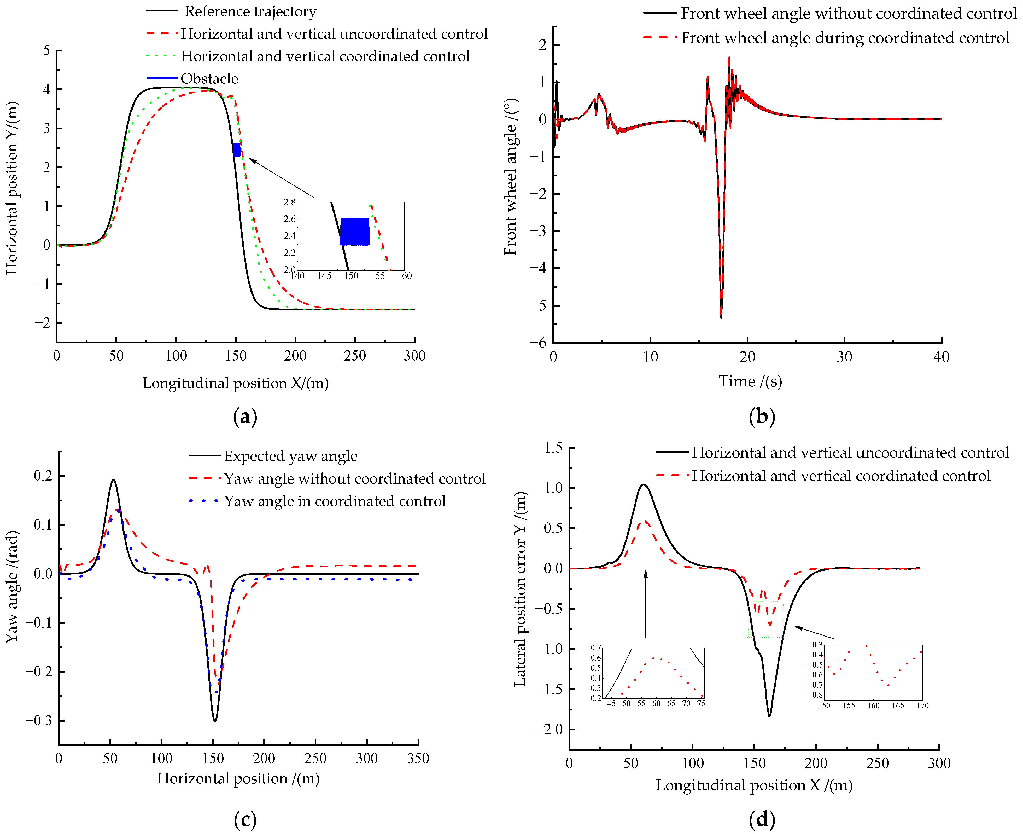
Under Condition 2, when unknown obstacles appear in the second half of the road, verification of obstacle avoidance replanning and trajectory tracking control of driverless ferry vehicles under double-shifted line conditions under coordinated control of horizontal and longitudinal controllers take place when the road adhesion coefficient is 0.8. Figure 25 illustrates the control algorithm’s simulation effect.

Figure 25.
Comparison of simulation results of control algorithms when the obstacle is behind. (a) Comparison between obstacle avoidance replanning and trajectory tracking. (b) Comparison of front wheel angle. (c) Comparison of yaw angle tracking effect. (d) Comparison of lateral position error.
From Figure 25a, we can see that, when the obstacle is in the second half of the road and there is no coordinated control in the horizontal and longitudinal directions, although the driverless ferry vehicle can avoid the obstacle, the tracking accuracy of the reference trajectory is poor. In horizontal and longitudinal coordinated control, the accuracy of the obstacle avoidance replanning and trajectory tracking reference trajectory of the driverless ferry vehicle is higher. From Figure 25b,c, we can see that the stability of the coordinated control of the horizontal and longitudinal motion of the driverless ferry vehicle is better than that of the uncoordinated control, and the precision of tracking the anticipated yaw angle is also effectively improved. From Figure 25d, observably, the greatest transverse position error is already close to 1.8 m when the driverless ferry uses uncoordinated control in the transverse and longitudinal directions. In contrast, the maximum transverse position error is reduced to about 0.7 m when using transverse–longitudinal coordinated control, which is 61.11% lower than the tracking error with transverse–longitudinal uncoordinated control. From the above analysis, we can see that the transverse and longitudinal coordinated control strategy designed has significantly improved the tracking effect of the ferry in obstacle avoidance replanning and trajectory tracking control. This demonstrates how well the coordinated control method works on both the horizontal and vertical axes.
6. Conclusions
The driverless ferry vehicle is the topic of this research. We studied how the too frequent acceleration- and braking-mode switching affects the comfort and stability of speed control for the ferry and designed the acceleration/braking switching module with an acceleration-tolerance interval. To study the problem of obstacle avoidance replanning and trajectory tracking control, a lateral motion controller with the function of obstacle avoidance replanning and the coordinated control of lateral motion and longitudinal motion were designed.
(1) Facing the problem of frequent switching between acceleration and braking modes of driverless ferry vehicles, a problem which affects the comfort and stability of speed control, according to the fuzzy control theory and PID control algorithm, the fuzzy PID longitudinal motion controller was designed, the braking control model was built, and the acceleration tolerance range of acceleration and braking was designed. It ensures the longitudinal speed tracking accuracy of the driverless ferry vehicle and the stability of the switching between acceleration and braking. (2) We were faced with the problem that the driverless ferry vehicle encounters unknown obstacles on the road, which affects the normal planning and tracking control of the vehicle, and ultimately causes the driverless ferry vehicle to be unable to drive normally. We performed a tire lateral deflection stiffness estimation using the vehicle dynamics model as a predictive model, based on which the lateral motion controller for the obstacle avoidance replanning function was designed. Transforming trajectory tracking becomes a secondary planning problem with constraints, and the obstacle avoidance function is designed by a point mass model and obstacle avoidance function. (3) For better tracking control, the speed-planning module predictive time-domain two-dimensional look-up table module was designed to coordinate the horizontal and longitudinal motion of the driverless ferry vehicle. The coordinated control offered by this method is shown in the simulation results; the planning and tracking effects of the driverless ferry vehicle were significantly improved, which validates the validity of the methodology devised in the paper.
To date, this work still has limitations. The coordinated control algorithm in this paper only carries out simulation experiments to verify its effectiveness, but it still needs to be verified in the real vehicle. Therefore, in the future research work, we can further confirm the effectiveness of the coordinated control algorithm in the real vehicle and analyze its control effect. And the potential practical impact of the scheme proposed in this paper is discussed. A further exploration of how these improvements mentioned in the scheme affect the overall ferry operation efficiency, passenger safety, and system reliability is needed.
Author Contributions
Conceptualization, X.L. and G.L.; methodology, X.L. and Z.Z.; software, Z.Z. and X.L.; validation, X.L., G.L., and Z.Z.; formal analysis, X.L.; investigation, Z.Z.; resources, G.L. and Z.Z.; data curation, X.L. and Z.Z.; writing—original draft preparation, X.L.; writing—review and editing, X.L. and G.L.; visualization, X.L. and Z.Z.; supervision, G.L.; project administration, G.L.; funding acquisition, G.L. All authors have read and agreed to the published version of the manuscript.
Funding
This work was supported by the General Program of the Natural Science Foundation of Liaoning Province in 2022 (2022-MS-376) and the Natural Science Foundation joint fund project (U22A2043).
Institutional Review Board Statement
Not applicable.
Informed Consent Statement
Not applicable.
Data Availability Statement
The original contributions presented in the study are included in the article, further inquiries can be directed to the corresponding author.
Conflicts of Interest
The authors declare no conflicts of interest.
References
- Yang, F.; Rao, Y. Vision-based intelligent vehicle road recognition and obstacle detection method. Int. J. Pattern Recognit. Artif. Intell. 2020, 34, 2050020. [Google Scholar] [CrossRef]
- Li, X.; Wang, L.; An, Y.; Huang, Q.-L.; Cui, Y.-H.; Hu, H.-S. Dynamic path planning of mobile robots using adaptive dynamic programming. Expert Syst. Appl. 2024, 235, 121112. [Google Scholar] [CrossRef]
- Li, Y.; Zhao, J.; Chen, Z.; Xiong, G.; Liu, S. A robot path planning method based on improved genetic algorithm and improved dynamic window approach. Sustainability 2023, 15, 4656. [Google Scholar] [CrossRef]
- Gao, H.; Song, X.; Gao, S. Research on Self-driving Vehicle Path Tracking Adaptive Method Based on Predictive Control. J. Phys. Conf. Ser. 2023, 2501, 012034. [Google Scholar] [CrossRef]
- Macadam, C.C. An Optimal Preview Control for Linear-Systems. J. Dyn. Syst.-Trans. ASME 1980, 102, 188–190. [Google Scholar] [CrossRef]
- MacAdam, C.C.; Johnson, G.E. Application of elementary neural networks and preview sensors for representing driver steering control behaviour. Veh. Syst. Dyn. 1996, 25, 3–30. [Google Scholar] [CrossRef]
- Li, S.; Xu, B.; Hu, M. Multi-point preview path tracking method for articulated vehicles based on dynamic model predictive control. Automot. Eng. 2021, 43, 1187–1194. [Google Scholar] [CrossRef]
- Li, W.; Yu, S.; Tan, L.; Li, Y.; Chen, H.; Yu, J. Integrated control of path tracking and handling stability for autonomous ground vehicles with four-wheel steering. Proc. Inst. Mech. Eng. Part D J. Automob. Eng. 2023. [Google Scholar] [CrossRef]
- Guo, J.; Luo, Y.; Li, K.; Guo, L. Adaptive dynamic surface longitudinal tracking control of autonomous vehicles. IET Intell. Transp. Syst. 2019, 13, 1272–1280. [Google Scholar] [CrossRef]
- Tang, C.; Zhao, Y.; Zhou, S. Research on trajectory tracking Control method of Intelligent vehicle. J. Northeast. Univ. (Nat. Sci. Ed.) 2020, 41, 1297. [Google Scholar] [CrossRef]
- Elias, G.H.S.; Al-Moadhen, A.; Kamil, H. Optimizing the PID controller to control the longitudinal motion of autonomous vehicles. AIP Conf. Proc. 2023, 2591, 040045. [Google Scholar] [CrossRef]
- Razmjooei, H.; Palli, G.; Nazari, M. Disturbance observer-based nonlinear feedback control for position tracking of electro-hydraulic systems in a finite time. Eur. J. Control 2022, 67, 100659. [Google Scholar] [CrossRef]
- Waschl, H.; Kolmanovsky, I.; Willems, F. Control Strategies for Advanced Driver Assistance Systems and Autonomous Driving Functions; Lecture Notes in Control and Information Sciences; Springer International: Cham, Switzerland, 2019; Volume 8. [Google Scholar] [CrossRef]
- Ye, N.; Wang, D.; Dai, Y. Enhancing Autonomous Vehicle Lateral Control: A Linear Complementarity Model-Predictive Control Approach. Appl. Sci. 2023, 13, 10809. [Google Scholar] [CrossRef]
- Paden, B.; Čáp, M.; Yong, S.Z.; Yershov, D.; Frazzoli, E. A survey of motion planning and control techniques for self-driving urban vehicles. IEEE Trans. Intell. Veh. 2016, 1, 33–55. [Google Scholar] [CrossRef]
- Zhao, Z.; Chang, H.; Wu, C. Adaptive Fuzzy Command Filtered Tracking Control for Flexible Robotic Arm with Input Dead-Zone. Appl. Sci. 2023, 13, 10812. [Google Scholar] [CrossRef]
- Ma, S.; Gong, P. Simulation and experiment of intelligent vehicle lateral control based on Fuzzy PID algorithm. In Proceedings of the 2023 IEEE International Conference on Control, Electronics and Computer Technology (ICCECT), Jilin, China, 28–30 April 2023; pp. 759–764. [Google Scholar] [CrossRef]
- Varshney, A.; Goyal, V. Re-evaluation on fuzzy logic controlled system by optimizing the membership functions. Mater. Today Proc. 2023. [Google Scholar] [CrossRef]
- Quan, L.; Chang, R.; Guo, C.; Li, B. Vehicle State Joint Estimation Based on Lateral Stiffness. Sensors 2023, 23, 8960. [Google Scholar] [CrossRef]
- Wang, W.; Li, G.; Liu, S.; Yang, Q. Trajectory Planning of a Semi-Trailer Train Based on Constrained Iterative LQR. Appl. Sci. 2023, 13, 10614. [Google Scholar] [CrossRef]
- Németh, B.; Gáspár, P. Hierarchical motion control strategies for handling interactions of automated vehicles. Control Eng. Pract. 2023, 136, 105523. [Google Scholar] [CrossRef]
- Li, S.; Ding, X. Intelligent vehicle trajectory Planning based on quintic Polynomials. J. Jiangsu Univ. (Nat. Sci. Ed.)/Jiangsu Daxue Xuebao (Ziran Kexue Ban) 2023, 44, 392–398. [Google Scholar] [CrossRef]
- Yu, L.; Wang, K.; Zhang, Q.; Zhang, J. Trajectory planning of a redundant planar manipulator based on joint classification and particle swarm optimization algorithm. Multibody Syst. Dyn. 2020, 50, 25–43. [Google Scholar] [CrossRef]
- Liu, X.; Liu, F.; Guo, J. Research on stability of high-speed autonomous vehicles based on linear time-varying model predictive control. Int. J. Veh. Des. 2023, 91, 360–383. [Google Scholar] [CrossRef]
- Wang, Y.; Li, J.; Wang, X.; Jin, C.; Yin, X. Development and Test of steering Angle measuring device for wheeled Tractor. J. China Agric. Univ. 2022, 27, 203–211. [Google Scholar] [CrossRef]
- Linden, M.; Eckstein, L.; Schlupek, M.; Duning, R. Influence of Wheel Bending Stiffness on Lateral Tire Characteristics. In Proceedings of the 12th International Munich Chassis Symposium 2021: Chassis Tech Plus, Munich, Germany, 29–30 June 2021; pp. 564–582. [Google Scholar] [CrossRef]
- Xia, Q.; Te, L.; Chen, L.; Xu, X.; Cai, Y. Vehicle Sideslip Angle Estimation Method Based on Redundant Information Fusion. Automot. Eng. 2022, 44, 280–289. [Google Scholar] [CrossRef]


Disclaimer/Publisher’s Note: The statements, opinions and data contained in all publications are solely those of the individual author(s) and contributor(s) and not of MDPI and/or the editor(s). MDPI and/or the editor(s) disclaim responsibility for any injury to people or property resulting from any ideas, methods, instructions or products referred to in the content. |
© 2024 by the authors. Licensee MDPI, Basel, Switzerland. This article is an open access article distributed under the terms and conditions of the Creative Commons Attribution (CC BY) license (https://creativecommons.org/licenses/by/4.0/).