Impacts of Variable Illumination and Image Background on Rice LAI Estimation Based on UAV RGB-Derived Color Indices

Abstract

Variations in illumination and image background present challenges for using UAV RGB imagery. Existing studies often overlook these issues, especially in rice. To separately evaluate the impacts of illumination variation and image background on rice LAI assessment, this study utilized Retinex correction and image segmentation to eliminate illumination variations and background effects, and then analyzed the changes in color indices and their relationship with LAI before and after implementing these methods separately. The results indicated that both Retinex correction and image segmentation significantly enhanced the correlation between color indices and LAI at different growth stages as well as the accuracy of constructing a multivariate linear regression model separately. Our analysis confirmed the significance of accounting for variation in illumination and rice field backgrounds in LAI analysis when using UAV RGB images. Illumination variation and image background elements significantly degrade the accuracy of LAI estimation.

1. Introduction

Rice is the main food crop for nearly 50% of the world’s population [1]. Considerable research has been devoted to improving rice yield and quality [2,3]. The leaf area index (LAI) is defined as the total one-sided area of leaf tissues per unit ground surface area [4]. Since the variation in LAI could reflect changes in crop growth rate, it has been widely used in biomass estimation and yield prediction of crops [5]. Hence, the precise and efficient estimation of crop LAI not only contributes to enhanced crop monitoring but also facilitates its utilization in comprehensive crop management and precision agriculture practices [6,7].

In recent years, the extensive application of unmanned aerial vehicles (UAVs) and RGB imagery in crop LAI research has been due to their cost-effectiveness, user-friendly processing, and high temporal and spatial resolution [8]. The most commonly used method in these applications is to estimate LAI based on color indices (CIs) obtained from RGB images [9]. Some studies suggest that CIs exhibit lower correlations with crop LAI [10], as they are easily affected by shadows and the incident angle of sunlight [11]. To enhance the accuracy of LAI estimation, researchers have employed various approaches. Some studies have shown that the near-infrared band possesses superior canopy inversion capability, and thus the use of multispectral cameras equipped with NIR bands could offer several advantages over the visible spectrum [12,13]. Research has also suggested that hyperspectral images could provide rich spectral features and detect subtle variations in crops, leading to improved accuracy in estimating the LAI compared to using the visible spectrum alone [14]. Qiao et al. [15] demonstrated that the fusion of vegetation indices and crop canopy morphological parameters effectively enhanced the estimation accuracy of LAI. However, previous studies have relied on simple linear or nonlinear relationships between CIs and LAI that may not fully capture the complexity of crop LAI and thus result in limited estimation accuracy [16]. Therefore, machine learning-based methods are commonly utilized to improve the estimation of LAI [10,17,18].

However, variation in illumination poses a significant challenge to the application of UAV imagery [19]. Variation in cloud cover and the inherent structural characteristics of crops are primary influencing factors on the variability in illumination [20,21,22]. The literature indicates that variation in illumination can significantly alter RGB images captured by UAV, hence affecting the application of CIs [23]. Therefore, it is imperative to perform illumination correction on the RGB images acquired from UAV [23]. However, existing research, particularly regarding the application of RGB-derived CIs, has shown limited consideration of methods such as light correction for reducing the impact of illumination variation on CIs [24]. This has constrained the accuracy of estimating crop phenotypic information based on CIs [25]. Therefore, color calibration is necessary to obtain reliable results [21]. Based on a recent literature review, only a minority of studies have employed color correction [25]. Thus, researchers have considered alternative approaches to overcoming the impact of variation in illumination by integrating texture, shape, and other features [26,27]. However, these approaches are unstable for many types of crop scenarios, including rice images obtained in complex field environments [26].

When studying crop phenotypes using CIs, another often-overlooked factor is the background of images, as this often limits the application of CIs [28]. The background elements of an image can be extracted through image segmentation [29,30]. One common method for crop image segmentation is to use CIs to separate crop and background by setting thresholds using different methods [31] that leverage the significant difference in CIs between crop and background pixels [29]. However, calculating CIs based on the average of the entire set of image pixels, rather than pixels of the crops, will inevitably lead to inaccurate results for the CIs, thereby causing overestimation or underestimation of phenotypic information [32,33]. For example, Liu et al. [12] discovered that a soil background heavily influenced the accuracy of maize LAI estimation. In a paddy field, apart from the soil, background elements may also include water, shadows, and weeds, which would interfere with the estimation of rice LAI [34]. Moreover, the background content of rice paddy images varies during different growth stages. During the tillering stage, the background elements include water, soil, weeds, and shadows [35,36]. In studies performed after the booting stage when rice plants have grown taller and formed a canopy, the background of the images has not been considered [31]. However, even at this stage, the presence of shadows in the images can have an impact on the estimation of crop traits [37].

Importantly, the influence of variation in illumination and image background on the derived vegetation indices from UAV RGB data analysis and evaluation has not been studied sufficiently [24,28]. Moreover, despite selecting sunny weather conditions for data collection [38], variation in illumination is inevitable due to differences in time and space during data acquisition. Therefore, RGB images obtained from UAVs will inevitably be affected. Additionally, the backgrounds of rice field images obtained during different growth stages and experimental sites may change. However, there remains a knowledge gap regarding the influence of variable illumination and image background on rice LAI estimation based on RGB-derived indices. The present study aims to fill this knowledge gap. Our primary objectives were to (1) assess the impact of variable illumination on rice LAI estimation based on CIs derived from UAV RGB images and (2) assess the impact of background on the estimation of LAI.

2. Materials and Methods

In analyzing the impact of variation in illumination on CIs and LAI estimation, we deviated from conventional approaches of studying CIs under different illumination conditions. This was because the usual methods do not align with the practicality of agricultural research, as UAV-based studies typically prioritize sunny weather conditions. During specific rice growth stages, the weather conditions may persistently remain overcast or partly cloudy. Therefore, we employed the automated multi-scale Retinex correction method to eliminate the influence of variable illumination on UAV images, resulting in corrected CIs that we named Retinex-corrected CIs. Then, we analyzed the changes in the original CIs and Retinex-corrected CIs. We investigated the variation in the relationship between CIs and LAI, assessed the response of CIs to variation in illumination, and examined the influence on LAI estimation. To assess the impact of the research background on CI and LAI, we segmented images into rice plants and background. The image segmentation adopted a method based on CIs and the Otsu threshold. To mitigate the impact of illumination on CIs that may result in significant errors in image segmentation, we opted for the Retinex-corrected CIs. We then proceeded to analyze the relationship between the Retinex-corrected CIs and LAI as well as the relationship between the Retinex-corrected CIs post-segmentation (segmented CIs) and LAI and examined how these relationships changed to evaluate the influence of the image background on LAI.

The overall workflow of the research is illustrated in Figure 1. The method comprises three steps: (1) data collection, including the collection of field and UAV-based data; (2) data processing, including generation of orthoimages, calculation of CIs, illumination correction, and image segmentation; and (3) statistical analysis, including correlation and regression analyses.

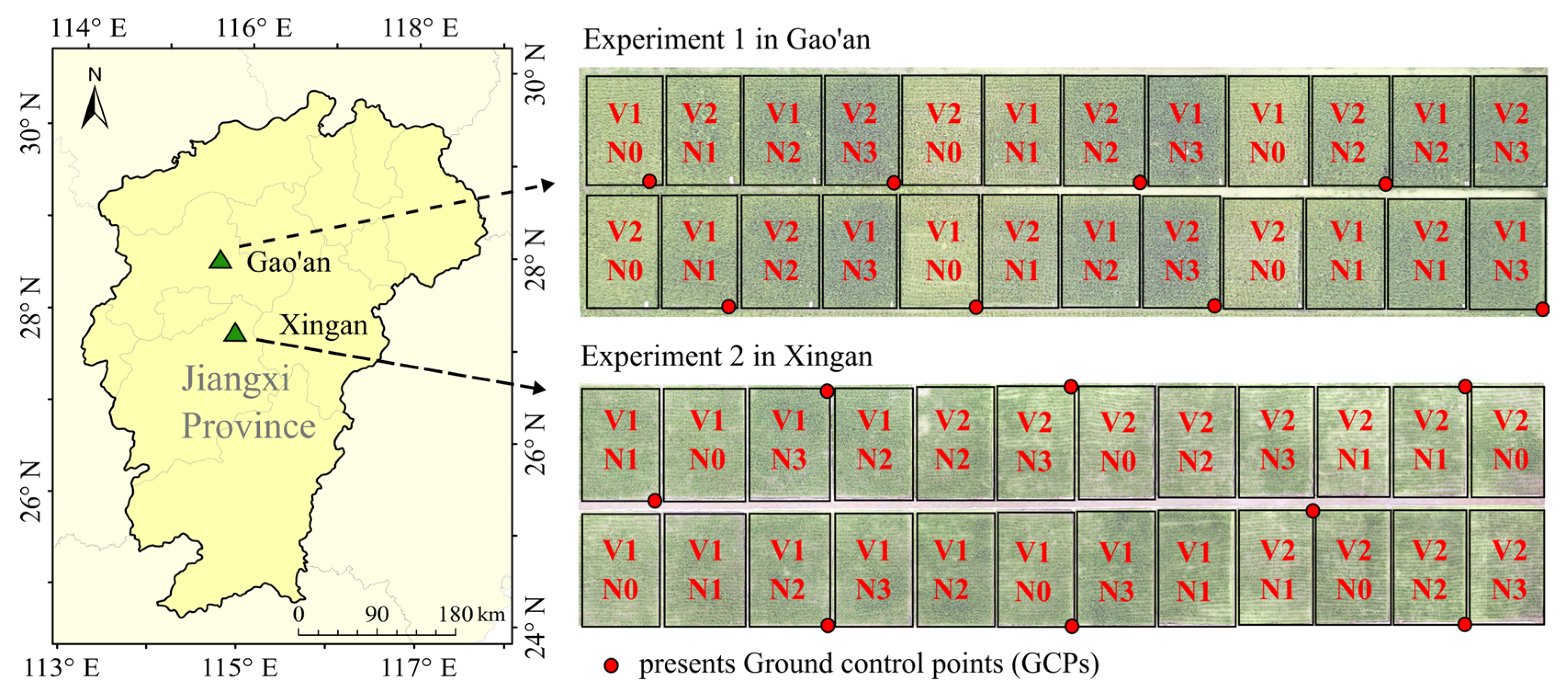
2.1. Site Description and Experimental Design

There were two experimental fields involved in this study located in Gao’an County (28°25′27″ N, 115°12′15″ E) and Xingan County (27°45′17.65″ N, 115°21′3.87″ E) in Jiangxi Province, China (Figure 2). Experiment 1 was performed at Gao’an, while Experiment 2 was performed at Xingan. Each experiment was carried out with four N treatments (0, 75, 150, and 225 kg N ha⁻¹, named N0, N1, N2, and N3), which were applied as 50% at the pre-planting stage, 30% at the tillering stage, and 30% at the booting stage. Phosphate fertilizer (60 kg ha⁻¹) was applied as a base fertilizer once, and potassium fertilizer (120 kg ha⁻¹) was applied together in the same proportions as for nitrogen fertilizer. Each experimental site design was divided into three replications for each treatment. Each experiment comprised 24 plots. Each plot covered an area of 30 m² (5 × 6 m) and was separated by ridges, covered with plastic film, and irrigated independently. Each plot had an independent irrigation or drainage system. The field management measures were the same as for the local high-yield field.

Experiment 1 was conducted in 2019 and 2020. The Japonica rice cultivars Xiangzaoxian 45 and Zaoxian 618 were planted. All rice cultivars were seeded on March 24 and transplanted to the paddy field on 23 April. Experiment 2 was conducted in 2019. The same rice varieties as in Experiment 1 were planted. All rice cultivars were seeded on 26 March and transplanted to the paddy field on 25 April. For geometric correction, each experiment utilized eight circular panels with a radius of 25 cm as ground control points (GCPs) (Figure 2). The GPS system (S-GNSS, China) was used to acquire position information of the GCPs.

2.2. Data Collection

2.2.1. UAV-Based Data Collection

We used a DJI Mavic 2 Pro UAV (DJI Sciences and Technologies Ltd., Shenzhen, China) with an RGB digital camera to acquire high-spatial-resolution rice images at a height of 10 m from the ground with a speed of 3 m/s. The forward and side overlap properties of the images were set to 80 and 70%, respectively. The flights were carried out in windless weather between 10:30 a.m. and 2:30 p.m. local time. The RGB images were captured from the tillering stage to the grouting stage. The specific observation periods and corresponding weather conditions are listed in

Table 1. Sampling dates and weather conditions of early rice in the fields.

Experiment	Location	Stage	Sampling Data	Weather Condition
Experiment 1 2019–2020	Gao’an	Tillering	11 May 2019	Sunny (not cloudy)
			11 May 2020	Partly cloudy
		Elongation	23 May 2019	Sunny (not cloudy)
			20 May 2020	Sunny (not cloudy)
		Booting	04 June 2019	Partly cloudy
			28 May 2020	Sunny (not cloudy)
		Heading	11 June 2019	Sunny (not cloudy)
			09 June 2019	Partly cloudy
		Grouting	22 June 2019	Partly cloudy
			23 June 2019	Partly cloudy
Experiment 2 2019	Xingan	Tillering	15 May 2019	Sunny (not cloudy)
		Elongation	22 May 2019	Partly cloudy
		Booting	03 June 2019	Partly cloudy
		Heading	11 June 2019	Partly cloudy
		Grouting	24 June 2019	Overcast

.

2.2.2. LAI Acquisition

Destructive sampling was used to collect rice LAI data in different plots. Repeated destructive sampling was carried out after RGB image acquisition. Four representative plants from each plot were brought back to the laboratory. The samples were separately divided into leaves and straw, and ten leaves were randomly selected from each sample. Middle segments of the selected leaves 8 cm in length were used to estimate leaf area (LA) by measuring the length and height. After the leaf area measurements, the middle segments of the selected leaves were initially dried for 30 min at 105 °C and then dried at 80 °C to a constant weight to acquire the dry matter quantity (DM₁). The specific leaf area (SLA) was calculated using Equation (1).

$$SLA=LA/{DM}_1$$

(1)

where LA is the total leaf area of ten leaves; SLA is the specific leaf area in cm²/g; and DM₁ is the dry matter quantity of ten leaves (g).

The remaining leaf blades were used to measure dry matter (DM₂). The leaf dry biomass of each plot (w) was obtained by summing DM₁ and DM₂. LAI was calculated using Equation (2).

$$LAI=1/4\times W\times SLA\times N\times {10}^{-4}$$

(2)

where LAI is the total leaf area per plot; W is the leaf dry biomass of each plot; and N is the number of rice plants in a surface of 1 m².

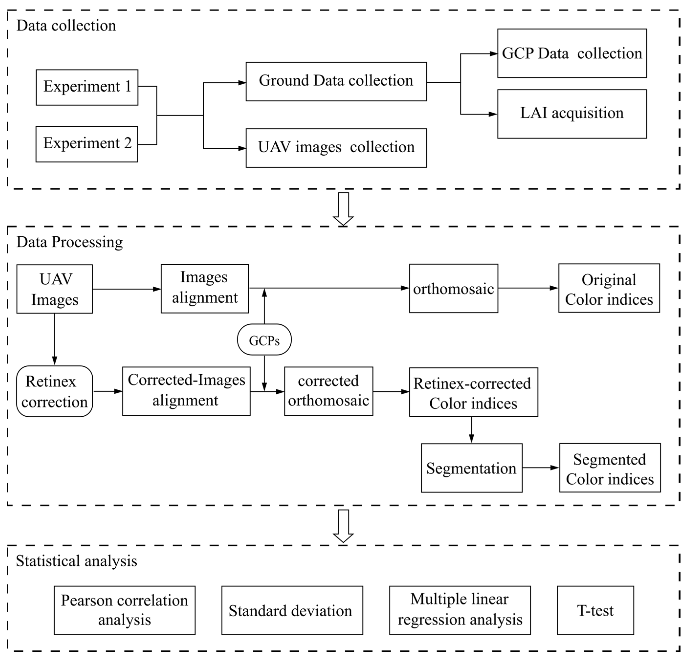
2.3. Data Processing

2.3.1. Image Mosaicking

Image mosaics of RGB images were first acquired using PhotoScan Software 1.4.5 (Agisoft LLC, St. Petersburg, Russia), and the images were saved in Tagged Image Format (TIF) files. The main processing workflow included image alignment, feature point matching, density point cloud generation, digital surface modeling (DSM), and orthophoto generation. Georeferencing was carried out in ArcGIS to unify the geographic reference system for all orthomosaic maps.

2.3.2. Illumination Correction

In this study, automated multi-scale Retinex was used for illumination correction. Retinex is a theoretical model of vision (Land, 1986) that has had a significant impact on adjusting unevenly illuminated color images. According to the Retinex theory, an image S(x,y) can be expressed as the product of an illumination image L(x,y) and a reflectance image R(x,y), as demonstrated in Equation (3).

$$S\left(x,y\right)=L\left(x,y\right)\times R\left(x,y\right)$$

(3)

A single-scale Retinex (SSR) image is obtained through a logarithmic transformation:

$$\ln R\left(x,y\right)=\ln S\left(x,y\right)-\ln \left[F\left(x,y\right)/S\left(x,y\right)\right]$$

(4)

where F(x,y) is a Gaussian surround function explicitly given by Equation (5):

$$F\left(x,y\right)=\lambda exp\left[-\left(x^2+y^2\right)/c^2\right]$$

(5)

the constant c is the scale parameter; λ is a constant matrix, and its values are determined by Equation (6).

$$\iint F\left(x,y\right)dxdy=1$$

(6)

The anti-logarithmic transformation of lnR(x,y) back to the real domain yields the corrected image.

A multi-scale Retinex (MSR) is obtained by taking the weighted sum of the SSR on multiple scales of an image using Equation (7):

$$S_i\left(x,y\right)=L_i\left(x,y\right)\times R_i\left(x,y\right)$$

(7)

transforming to the logarithmic domain,

$$\ln R\left(x,y\right)=\sum _k^K{\omega }_k\left\{\ln S\left(x,y\right)-\ln \left[F\left(x,y\right)⨂S\left(x,y\right)\right]\right\}$$

(8)

where K is the number of Gaussian surround functions and ω_k is the weight of the k-th SSR; ⨂ represents multiplication by elements.

Automatic multi-scale Retinex correction starts by applying bilateral filtering to an input-enhanced image for noise reduction. Then, the image is transformed to the logarithmic domain for MSR enhancement. The resulting image is then automatically color-corrected using a dynamic range adjustment. Finally, the image is transformed back to the spatial domain to obtain a final enhanced image. The study by Wang et al. [23] contains the specific steps and parameter settings.

2.3.3. Color Indices

In this study, UAV RGB images of the five growth stages were used to study the relationship between LAI and image features. Based on previously published results and the relationship between image features and LAI, 25 commonly used color indices involving different color spaces such as RGB, HSV, and CIE L*a*b* were extracted from RGB images [13,35]. Detailed information for the color indices is listed in

Table 2. Definition and description of the RGB-CIs used in this study.

Index	Name	Definition	Reference
C1	Color index of vegetation extraction (CIVE)	0.441R − 0.881G + 0.385B + 18.78745	[31]
C2	Combination of green 1 (COM1)	ExG + CIVE + ExGR + VEG	[29]
C3	Combination of green 2 (COM2)	0.36ExG + 0.47CIVE + 0.17VEG	[29]
C4	Excess green (EXG)	2G − B − R	[29]
C5	Excess green minus excess red (EXGR)	3G − 2.4R − B	[29]
C6	Excess red (EXR)	1.4R-G	[29]
C7	Green leaf index (GLI)	(2G − R − B)/(2G + R+ B)	[39]
C8	Green minus red index (GMR)	G − R	[34]
C9	Color intensity index (INT)	(R + G + B)/3	[34]
C10	L* component of CIE L*a*b* color spaces	L*
C11	Modified excess green index (MExG)	1.262G − 0.884R − 0.311B	[40]
C12	Modified green–red vegetation index (MGRVI)	(G2 − B2)/(G2 + B2)	[41]
C13	Normalized blueness intensity (NBI)	B/(R + G + B)	[34]
C14	Normalized difference index (NDI)	128((G − R)/(G + R) + 1)	[42]
C15	Normalized difference L*b* index (NDLBI)	(L* − b*)/(L* + b*)	[43]
C16	Normalized green–blue difference index (NGBDI)	(G − B)/(G + B)	[44]
C17	Normalized greenness intensity (NGI)	G/(R + G + B)	[34]
C18	Normalized redness intensity (NRI)	R/(R + G + B)	[34]
C19	Red–green–blue vegetation index (RGBVI)	(G2 − RB)/(G2 + RB)	[41]
C20	Saturation (S)	S
C21	Value refers to the brightness of the color	V
C22	Visible atmospherically resistant index (VARI)	(G − R)/(G + R − B)	[45]
C23	Vegetative index (VEG)	G/(RαB(1 − α))	[46]
C24	a* component of CIE L*a*b* color spaces	a*
C25	b* component of CIE L*a*b* color spaces	b*

.

2.3.4. Image Segmentation

Based on our previous research, we opted to utilize MxEG for image segmentation [35]. For thresholding in the image segmentation process, we chose to employ Otsu’s thresholding method. Otsu’s algorithm is unaffected by image brightness and contrast and is computationally simple, making it one of the best choices for threshold selection in image segmentation [29]. The Otsu algorithm determines the optimal threshold value based on the grayscale characteristics of an image, maximizing the between-class variance between the target and background regions.

The Otsu threshold is calculated by first stretching the image to a range of 0–255. The parameter p_i represents the probability of occurrence of pixel value i occurring. Suppose there exists a threshold k that divides the image into two classes C₀ and C₁, maximizing the inter-class variance σ². C₀ consists of pixels with levels [0, …, k], and C₁ consists of pixels with levels [k + 1, …, 255]. Let p₀(k), p₁(k) represent the probabilities of C₀ and C₁, respectively. Similarly, let u₀(k), u₁(k) denote the means of C₀ and C₁.

These values are given by:

$$p_0\left(k\right)=\sum _{i=0}^k{p}_i$$

(9)

$$p_1\left(k\right)=\sum _{i=k+1}^{255}{p}_i=1-p_0\left(k\right)$$

(10)

$$u_0\left(k\right)=\sum _{i=0}^k\frac{i{p}_i}{p_0\left(k\right)}$$

(11)

$$u_1\left(k\right)=\sum _{i=k+1}^{255}\frac{i{p}_i}{p_1\left(k\right)}$$

(12)

The between-class variance σ²(k) is given by:

$${\sigma }^2\left(k\right)=p_0\left(k\right){u_0}^2\left(k\right)+p_1\left(k\right){u_1}^2\left(k\right)$$

(13)

When σ²(k) reaches its maximum, k is the optimal threshold value:

$$k=arg\underset{0<k<255}{\max }{\sigma }^2\left(k\right)$$

(14)

The steps involved in this image segmentation are as follows.

Step 1. MxEG values are used to replace the original image gray values. The new gray value histogram relative to the original image histogram has a more bimodal distribution and is suitable for the Otsu method.

Step 2. The Otsu method is used to find the optimal segmentation threshold value.

Step 3. UAV images are then divided into rice and background regions by the optimal threshold value.

2.4. Statistical Analysis

Python was used for statistical analyses. Pearson correlation coefficients for LAI and CIs were calculated by the function scipy.stats.pearsonr. Analysis of the standard deviation (SD) was used to compare experimental groups using the function scipy.stats.mstats.f_oneway. To mitigate the impact of machine learning algorithms on the research results, multiple linear regression analysis was utilized to explore the estimation of LAI based on CIs. Multivariate linear regression was implemented using the LinearRegression function from the scikit-learn library. The impact of variation in illumination and image background elements on LAI estimation was analyzed by the LinearRegression function.

3. Results

3.1. Effects of Illumination on the Estimation of LAI

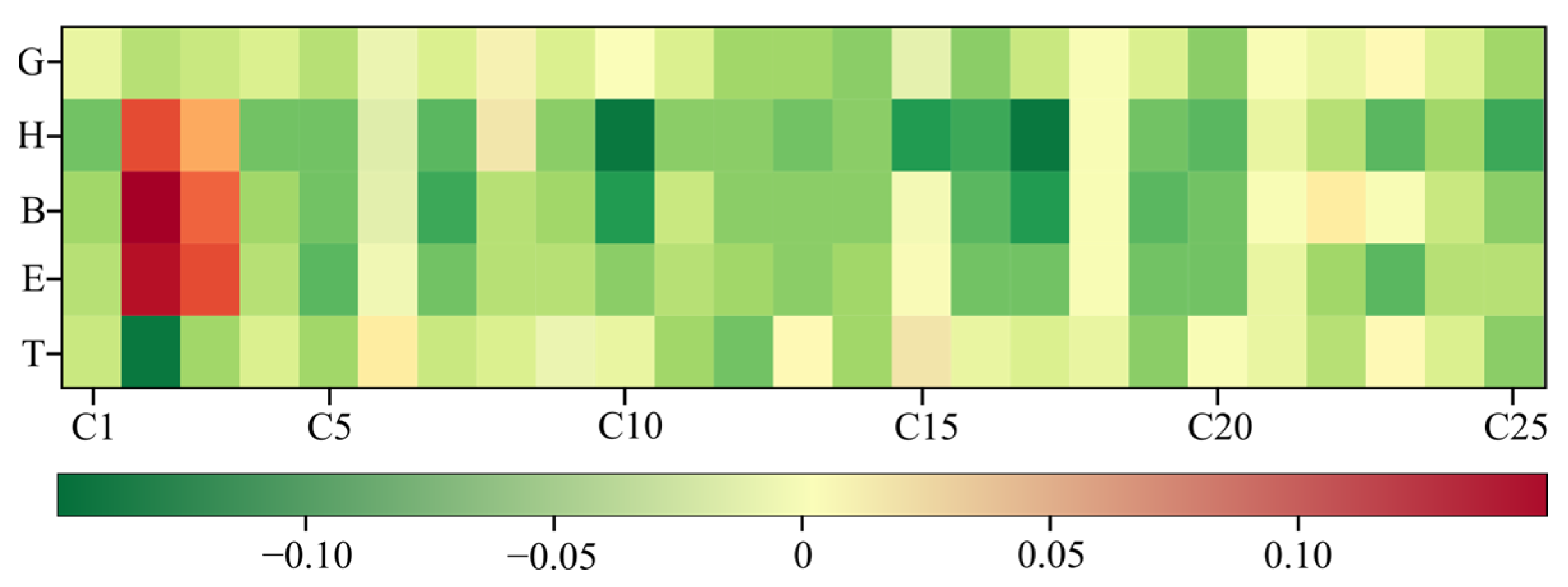
3.1.1. The Impact of Variable Illumination on CIs

To analyze the impact of variable illumination on CIs from RGB images, Retinex correction was implemented on UAV images collected at five growing stages. We then analyzed changes in the SDs of original CIs and Retinex-corrected CIs. Figure 3 presents changes in the SDs of 25 CIs at five growth stages. There was a significant reduction in the SDs of CIs in the images of each growth stage after undergoing Retinex correction in comparison to the original images, indicating that Retinex correction reduced the diversity of data. The results demonstrated that illumination conditions have a significant influence on CIs. For example, the SD of the C1 for different growth stages showed a noticeable decrease (Figure 3). The decrease in SD for C1 suggests that variation in illumination conditions during the growth stages can lead to anomalous data and thus can have a negative impact on estimating crop phenotypes using CIs. Simultaneously, the SD of CIs also exhibited variation across different growth stages. Specifically, there was relatively low variability in CI changes at the tillering and grouting stages, while there was greater variability during the elongation, booting, and heading stages. Only C6, C18, and C21 exhibited relatively small variations during the entire growth period of early rice (Figure 3). The variances of other CIs such as C8 showed relatively small changes only at the tillering and elongation stages.

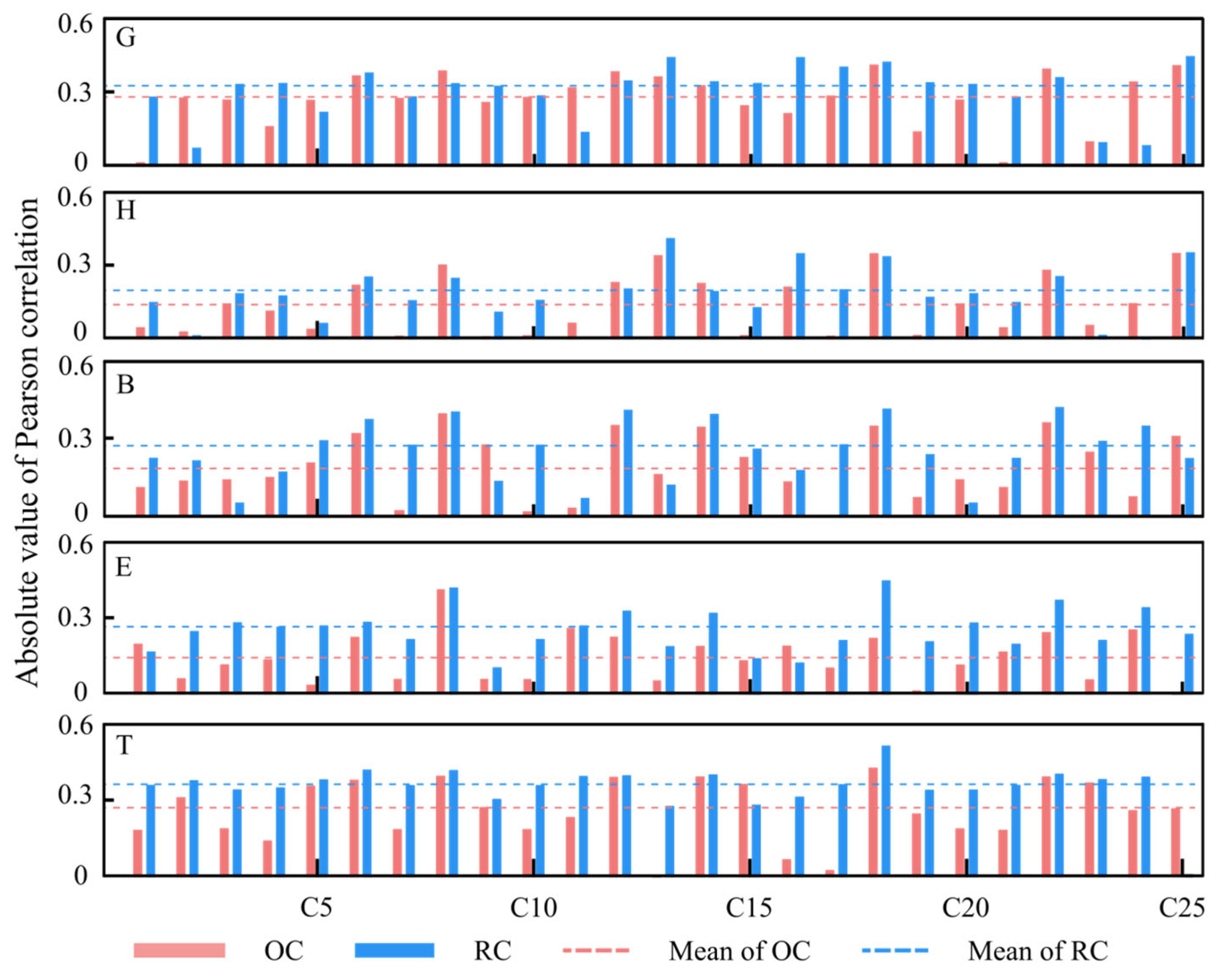
3.1.2. Correlation Analysis of CIs and LAI

To further examine the impact of illumination on CIs, Pearson correlations were calculated between different CIs and LAI values at the various growth stages (Figure 4). The average Pearson correlation coefficient between the original CIs and LAI was lower than that between the Retinex-corrected CI and LAI. Retinex correction improved the correlation between CIs and LAI. Taking the tillering stage as an example, the average correlation between the original CI and LAI was 0.27, whereas, after Retinex correction, the value increased to 0.36. Retinex correction resulted in an increase of 0.12 in the correlation between the CIs and LAI at the elongation stage. This fully demonstrated that variation in illumination conditions during growth stages can have a negative impact on CIs for LAI research. Considering the entire growth period, correlations between CIs and LAI were significantly higher in the tillering and grouting stages compared to the jointing, booting, and heading stages. Meanwhile, C8, C18, and C22 had relatively high correlations with LAI (Figure 4). C18 showed minimal changes in correlations with LAI after Retinex correlation, indicating that it was less affected by variation in illumination compared to other CIs. The correlation between C8 and LAI showed no significant changes at the tillering, jointing, or booting stages, but there were significant changes at the heading and grouting stages, consistent with the response of C8 to variation in illumination.

3.1.3. Estimation of LAI by Regression Analysis of CIs

We selected five CIs with the highest correlations with LAI and intercorrelations below 0.8 to construct a multiple linear regression model to further examine the impact of illumination on LAI estimation. The performance of the models is shown in

Table 3. Coefficient of determination (R²) of the multiple linear regression model between the different CIs and LAI.

Stage	Original CIs	Retinex-Corrected CIs	Segmented CIs
Tillering	0.47	0.57	0.64
Elongation	0.31	0.50	0.58
Booting	0.38	0.52	0.63
Heading	0.33	0.51	0.60
Grouting	0.46	0.55	0.61

. In the tillering stage, the R² value of the model based on the original CIs was 0.47, while the model based on Retinex-corrected CIs achieved an R² of 0.57. Retinex correction effectively improved the accuracy of the LAI estimation model. Similar observations were made at other stages. These results indicated that variation in illumination significantly affected the performance of the rice LAI estimation model. Moreover, the performance of the estimation model was subpar when the images captured by unmanned aerial vehicles were not subject to illumination correction.

3.2. Effects of the Background on LAI Estimation

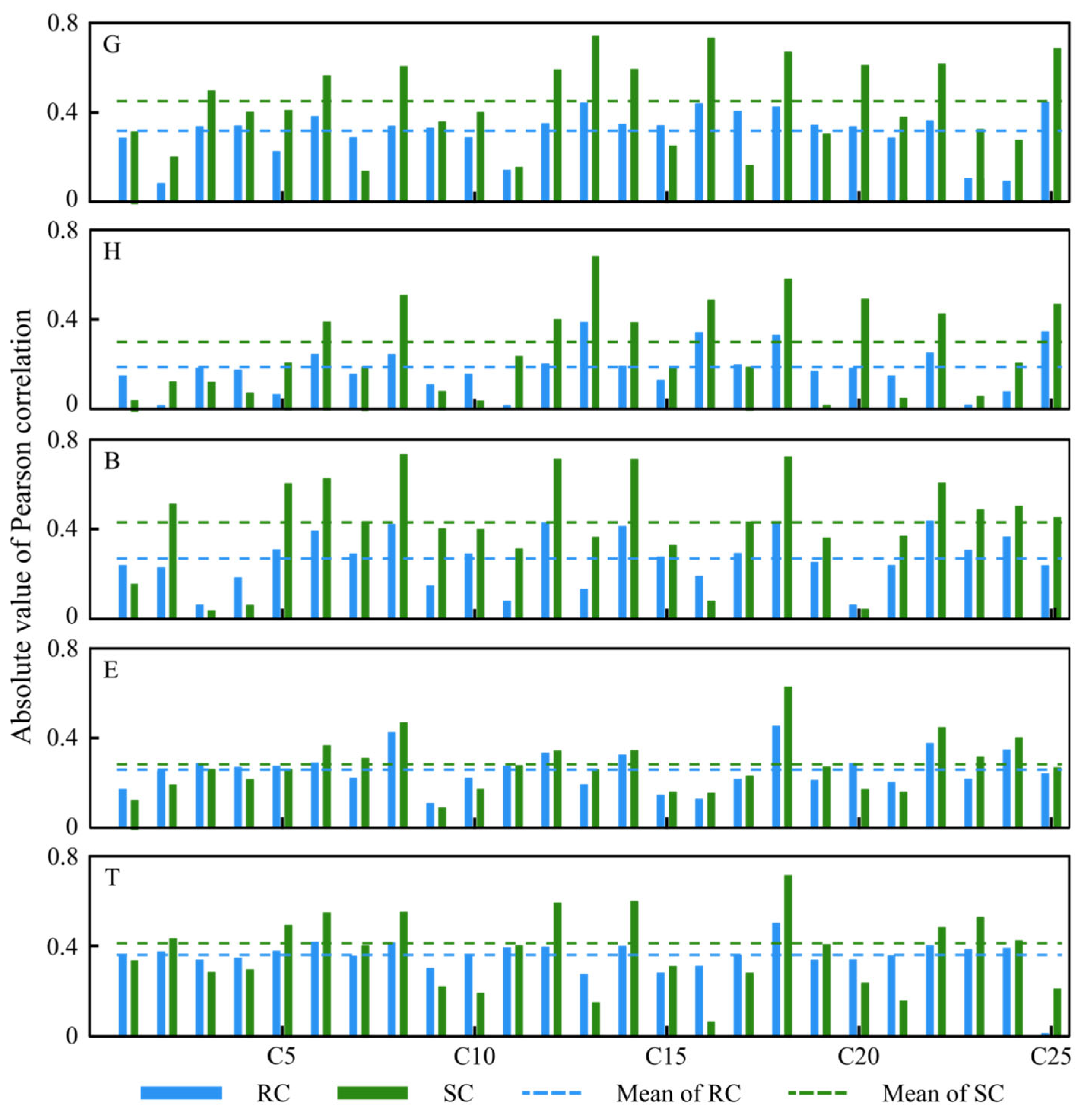
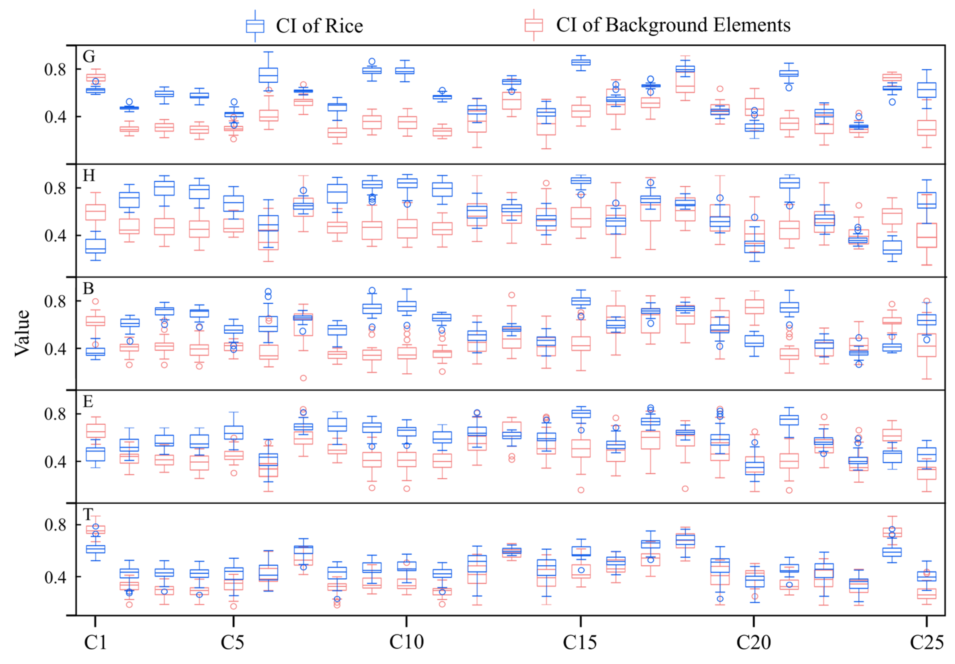
3.2.1. The Impact of Background on CIs

To investigate the impact of background on CIs, we employed image segmentation techniques to separate the Retinex-corrected images into rice plants and backgrounds. By analyzing the changes in CIs before and after segmentation, we could assess the influence of background on the CIs of the rice fields. Figure 5 presents a boxplot of the CIs of rice and background. There were significant differences between the CIs of rice and background. This indicated that segmenting images into rice and background reduces the range of CI variation compared to non-segmented images. We further analyzed the difference in CI between rice and background using a t-test, and the results are presented in

Table 4. Comparisons of the CIs difference between rice and image background using t-tests.

CIs	Tillering	Elongation	Booting	Heading	Grouting
C1	−8.098 **	−9.641 **	−6.951 **	−6.716 **	−9.719 **
C2	6.007 **	7.835 **	6.148 **	5.495 **	5.118 **
C3	8.574 **	9.865 **	6.839 **	6.859 **	8.886 **
C4	8.509 **	9.723 **	6.708 **	6.848 **	9.78 **
C5	4.415 **	6.435 **	3.805 **	3.956 **	2.036 *
C6	1.146	2.145*	3.434 **	4.195 **	5.179 **
C7	4.550 **	3.508 **	1.506	0.467	1.531
C8	6.083 **	8.847 **	7.583 **	5.725 **	3.827 **
C9	3.470 **	6.568 **	6.847 **	7.080 **	11.185 **
C10	4.101 **	7.181 **	6.842 **	7.081 **	11.044 **
C11	8.716 **	10.317 **	8.399 **	7.581 **	11.303 **
C12	3.265 **	3.46 **	1.1	0.372	0.159
C13	2.473 *	1.221	1.396	1.406 **	1.885 **
C14	3.051 **	2.369 *	0.776	−0.168	−0.142
C15	4.823 **	6.638 **	6.464 **	6.176 **	11.352 **
C16	2.866 **	2.526 *	−1.233	−0.464	−2.390 *
C17	3.266 **	6.471 **	1.894	2.143 *	2.793 **
C18	0.738	2.615 *	1.868	2.163 *	2.042 *
C19	3.106 **	3.173 **	−3.21 **	−0.691	−3.752 **
C20	−1.984	0.038	−7.274 **	−3.552 **	−5.415 **
C21	4.224 **	7.565 **	7.312 **	7.655 **	11.146 **
C22	2.900 **	1.106	0.622	0.062	−0.044
C23	1.620 **	0.146	−2.257 **	−1.955	−3.755 **
C24	−7.669 **	−9.385 **	−8.219 **	−6.752 **	−9.043 **
C25	7.467 **	8.009 *	8.170 **	3.564 **	4.443 **

The ** behind a number indicates that the correlation was significant at p < 0.01; * indicates significant at p < 0.05.

. Significant differences were observed between rice and background in most CIs. At the tillering stage, the pixel values of rice plants and background pixels showed no significant differences except for C6, C18, and C20. At the booting, heading, and filling stages, significant differences were observed in C7, C12, C14, and C22.

3.2.2. Correlation Analysis between CIs and LAI

To further analyze the influence of background elements on the relationship between CIs and LAI, we compared the Pearson correlations between CIs and LAI before and after image segmentation in key growth stages. Figure 6 presents the Pearson correlation trends between different CIs and LAI values at different growth stages. The Pearson correlation coefficients between segmented CIs and LAI were significantly higher than Retinex-corrected CIs. This indicated that image segmentation significantly improved the correlation between CIs and LAI. Taking the heading stage image as an example, the average Pearson coefficient between Retinex-corrected CIs and LAI was 0.27. After image segmentation, the correlation coefficient increased to 0.43, with an increase of 0.16. This demonstrated that image background plays a counteractive role in the estimation of LAI by CIs. Additionally, we found that after image segmentation, the correlation between CIs and LAI increased notably at the booting, heading, and filling stages.

3.2.3. Estimation of LAI by Regression Analysis of CIs

Similar to Section 3.2.3, we also opted to use three CIs to construct a multiple linear model and assess the impact on image segmentation for LAI evaluation. The performance of the models is shown in Table 2. Across all growth stages, the model based on the segmented CIs exhibited the highest R² values compared to the model based on the original CIs and original images and the model based on Retinex-corrected CIs. This indicated that image segmentation effectively enhanced the accuracy of LAI simulation and highlighted the significant impact of background elements on LAI estimation. Compared to the Retinex-corrected CI models, the R² value of segmented CI models in the tillering and heading stages showed the greatest improvement, with an increase of 0.11. The segmented CI models for the jointing stage showed the least increase at only 0.04. Overall, image segmentation enhanced the estimation accuracy of LAI. Background elements can have significant effects on the estimation of LAI by CIs.

4. Discussion

4.1. Influence of Illumination on the Estimation of LAI

CIs that use ratios between color channels are theoretically stable under variable illumination [22], and they are designed to cope with the variability of natural daylight illumination [46,47]. However, our results were not consistent with this statement. After Retinex correction, there were significant increases in the correlations between CIs and LAI and the R2 values of the multiple regression models at all growth stages (Figure 4; Table 3). This demonstrated that variable illumination could have a significant impact on CIs. Similarly, Wang et al. [23] found that RGB-derived CIs were substantially affected by variable illumination. This is primarily because when cloud cover reduces the amount of direct sunlight, the phenomenon of light scattering becomes more prominent at shorter wavelengths compared to longer wavelengths [48]. This has varying effects on different color channels that in turn affect RGB-derived CIs [23]. This could be the reason why, in our study, there were low correlations between LAI and CIs related to the blue channel except for C18.

Therefore, it is necessary to select CIs based on specific conditions, and illumination correction is a crucial step for processing and application of RGB images. We found that CIs with strong resistance to illumination variation were not highly correlated with LAI. Hence, when choosing CIs to estimate LAI, it is important not to focus solely on their robustness to variation in illumination. Meanwhile, unlike Wang et al. [23], C7, C16, and C19 in our study performed less effectively in dealing with variation in illumination compared to C6 and C18. Due to the variation in cloud cover, the amount of transmitted blue light also differs [49], in turn significantly affecting the performance of the mentioned indices. Consequently, there is a reduced correlation between these indices and the LAI.

When considering the entire growth period, we observed that after Retinex correction, the correlation between CIs and LAI showed the greatest enhancement at the jointing stage, while the improvement was relatively minimal during the grouting stage. Similar results were obtained from the regression analysis. After Retinex correction, the R² value of the multiple regression model at the elongation stage showed the largest improvement, while showing the least improvement at the grouting stage (Table 3). This could likely be attributed to the fact that at the elongation stage of the study area for early rice, there is largely cloudy weather. The variable illumination during UAV flights leads to spatial discrepancies in the color rendition of the captured images. This affects the correlation between CIs and LAI as well as the accuracy of the regression model. Retinex correction can effectively address this issue, thereby improving the correlations between CIs and LAI as well as the accuracy of the model [23]. In contrast, at the grouting stage, the color of the canopy gradually transitions from green to yellow. This is due to the inherent absorption and reflection characteristics of yellow objects, resulting in less variation in wavelength, as the perception of color in yellow objects is less affected by changes in illumination compared to green objects. Therefore, illumination plays a significant role in the estimation of LAI, and it is necessary to perform illumination correction when conducting LAI research with UAVs.

4.2. Influence of the Background on LAI Estimation

Image segmentation can enhance the accuracy of LAI estimation (Figure 6; Table 4). Paddy field image segmentation refers to the process of categorizing the pixels in an image into rice and background. CIs are calculated by the average of the entire set of pixels in images. The background can contribute to the overall gap fraction when mixed with the rice. This mixing effect can lead to underestimation or overestimation of LAI if not properly accounted for [50]. After segmenting the image into rice and background, only the rice pixels were considered for the calculation of CIs. The background elements of paddy field images include soil, water, reflections of rice plants, and weeds. The CIs of the background exhibited significant differences from the CIs of crops [29].

The correlations between segmented CIs and LAI at the tillering and jointing stages increased less compared to the booting, heading, and grouting stages. Due to the uneven growth of our experimental rice plants, soil, weeds, and shade are still observable in the images taken after the booting stage. The background elements in paddy field images of reproductive stages largely consist of soil and weeds, making the background relatively simple. This results in a higher accuracy of image segmentation. In contrast, the background elements at the tillering and elongation stages are more complex, including water, water hyacinth, and shadows [35]. This complexity leads to lower segmentation accuracy in the images of these two growth stages [37], ultimately affecting the correlations between CIs and LAI as well as the accuracy of the models. From the holistic perspective of the entire growth period, image segmentation can effectively enhance the accuracy of LAI estimation.

After correction for illumination and image segmentation, the correlation of CIs at various growth stages from tillering to grouting stages was significantly improved. The multiple linear models built for the elongation and heading stages showed increases in R² of up by 0.27 (Table 3). This demonstrates the significant impact of illumination variations and image backgrounds on the estimation of rice LAI.

5. Conclusions

The present work showed that the estimation of rice LAI using CIs derived from UAV RGB images was strongly influenced by variations in illumination and the image background. The variation in illumination resulted in changes in image colors, making it challenging to compare crop phenotypic traits over time and space. However, employing multi-scale Retinex correction could mitigate the impact of variable illumination on CIs and improve the accuracy of LAI estimation. Because CIs were calculated based on the average values of the entire image, rice plants combined with the background could lead to underestimation or overestimation of rice LAI without proper segmentation. Overall, our analysis confirmed the significance of accounting for variation in illumination and rice field backgrounds in LAI analysis using UAV RGB images. These findings underscored the importance of image processing techniques in enhancing the utility of UAV RGB images in agricultural phenotyping. Furthermore, this study provided a method to improve the accuracy of LAI estimation based on UAV RGB images.

References

1. Muthayya, S.; Sugimoto, J.D.; Montgomery, S.; Maberly, G.F. An Overview of Global Rice Production, Supply, Trade, and Consumption. Ann. N. Y. Acad. Sci. 2014, 1324, 7–14. [Google Scholar] [CrossRef] [PubMed]
2. Ren, D.; Ding, C.; Qian, Q. Molecular Bases of Rice Grain Size and Quality for Optimized Productivity. Sci. Bull. 2023, 68, 314–350. [Google Scholar] [CrossRef] [PubMed]
3. Peng, S.; Khush, G.S.; Virk, P.; Tang, Q.; Zou, Y. Progress in Ideotype Breeding to Increase Rice Yield Potential. Field Crops Res. 2008, 108, 32–38. [Google Scholar] [CrossRef]
4. Bréda, N.J.J. Ground-based Measurements of Leaf Area Index: A Review of Methods, Instruments and Current Controversies. J. Exp. Bot. 2003, 54, 2403–2417. [Google Scholar] [CrossRef]
5. Xu, J.; Quackenbush, L.J.; Volk, T.A.; Im, J. Forest and Crop Leaf Area Index Estimation Using Remote Sensing: Research Trends and Future Directions. Remote Sens. 2020, 12, 2934. [Google Scholar] [CrossRef]
6. Liu, X.; Cao, Q.; Yuan, Z.; Liu, X.; Wang, X.; Tian, Y.; Cao, W.; Zhu, Y. Leaf Area Index Based Nitrogen Diagnosis in Irrigated Lowland Rice. J. Integr. Agric. 2018, 17, 111–121. [Google Scholar] [CrossRef]
7. Ilniyaz, O.; Du, Q.; Shen, H.; He, W.; Feng, L.; Azadi, H.; Kurban, A.; Chen, X. Leaf Area Index Estimation of Pergola-Trained Vineyards in Arid Regions Using Classical and Deep Learning Methods Based on UAV-Based RGB Images. Comput. Electron. Agric. 2023, 207, 107723. [Google Scholar] [CrossRef]
8. Maes, W.H.; Steppe, K. Perspectives for Remote Sensing with Unmanned Aerial Vehicles in Precision Agriculture. Trends Plant Sci. 2019, 24, 152–164. [Google Scholar] [CrossRef] [PubMed]
9. Istiak, M.A.; Syeed, M.M.M.; Hossain, M.S.; Uddin, M.F.; Hasan, M.; Khan, R.H.; Azad, N.S. Adoption of Unmanned Aerial Vehicle (UAV) Imagery in Agricultural Management: A Systematic Literature Review. Ecol. Inform. 2023, 78, 102305. [Google Scholar] [CrossRef]
10. Yamaguchi, T.; Tanaka, Y.; Imachi, Y.; Yamashita, M.; Katsura, K. Feasibility of Combining Deep Learning and RGB Images Obtained by Unmanned Aerial Vehicle for Leaf Area Index Estimation in Rice. Remote Sens. 2020, 13, 84. [Google Scholar] [CrossRef]
11. Bouguettaya, A.; Zarzour, H.; Kechida, A.; Taberkit, A.M. Deep Learning Techniques to Classify Agricultural Crops through UAV Imagery: A Review. Neural Comput. Appl. 2022, 34, 9511–9536. [Google Scholar] [CrossRef] [PubMed]
12. Liu, S.; Jin, X.; Nie, C.; Wang, S.; Yu, X.; Cheng, M.; Shao, M.; Wang, Z.; Tuohuti, N.; Bai, Y.; et al. Estimating Leaf Area Index Using Unmanned Aerial Vehicle Data: Shallow vs. Deep Machine Learning Algorithms. Plant Physiol. 2021, 187, 1551–1576. [Google Scholar] [CrossRef]
13. Qiu, Z.; Ma, F.; Li, Z.; Xu, X.; Du, C. Development of Prediction Models for Estimating Key Rice Growth Variables Using Visible and NIR Images from Unmanned Aerial Systems. Remote Sens. 2022, 14, 1384. [Google Scholar] [CrossRef]
14. Gong, Y.; Yang, K.; Lin, Z.; Fang, S.; Wu, X.; Zhu, R.; Peng, Y. Remote Estimation of Leaf Area Index (LAI) with Unmanned Aerial Vehicle (UAV) Imaging for Different Rice Cultivars throughout the Entire Growing Season. Plant Methods 2021, 17, 88. [Google Scholar] [CrossRef] [PubMed]
15. Qiao, L.; Gao, D.; Zhao, R.; Tang, W.; An, L.; Li, M.; Sun, H. Improving Estimation of LAI Dynamic by Fusion of Morphological and Vegetation Indices Based on UAV Imagery. Comput. Electron. Agric. 2022, 192, 106603. [Google Scholar] [CrossRef]
16. Verrelst, J.; Camps-Valls, G.; Muñoz-Marí, J.; Rivera, J.P.; Veroustraete, F.; Clevers, J.G.P.W.; Moreno, J. Optical Remote Sensing and the Retrieval of Terrestrial Vegetation Bio-Geophysical Properties—A Review. ISPRS J. Photogramm. Remote Sens. 2015, 108, 273–290. [Google Scholar] [CrossRef]
17. Guo, X.; Wang, R.; Chen, J.M.; Cheng, Z.; Zeng, H.; Miao, G.; Huang, Z.; Guo, Z.; Cao, J.; Niu, J. Synergetic Inversion of Leaf Area Index and Leaf Chlorophyll Content Using Multi-Spectral Remote Sensing Data. Geo-Spat. Inf. Sci. 2023, 1–14. [Google Scholar] [CrossRef]
18. Jiang, J.; Johansen, K.; Stanschewski, C.S.; Wellman, G.; Mousa, M.A.A.; Fiene, G.M.; Asiry, K.A.; Tester, M.; McCabe, M.F. Phenotyping a Diversity Panel of Quinoa Using UAV-Retrieved Leaf Area Index, SPAD-Based Chlorophyll and a Random Forest Approach. Precis. Agric. 2022, 23, 961–983. [Google Scholar] [CrossRef]
19. Burdziakowski, P.; Bobkowska, K. UAV Photogrammetry under Poor Lighting Conditions—Accuracy Considerations. Sensors 2021, 21, 3531. [Google Scholar] [CrossRef]
20. Arroyo-Mora, J.P.; Kalacska, M.; Løke, T.; Schläpfer, D.; Coops, N.C.; Lucanus, O.; Leblanc, G. Assessing the Impact of Illumination on UAV Pushbroom Hyperspectral Imagery Collected under Various Cloud Cover Conditions. Remote Sens. Environ. 2021, 258, 112396. [Google Scholar] [CrossRef]
21. Hassanijalilian, O.; Igathinathane, C.; Doetkott, C.; Bajwa, S.; Nowatzki, J.; Haji Esmaeili, S.A. Chlorophyll Estimation in Soybean Leaves Infield with Smartphone Digital Imaging and Machine Learning. Comput. Electron. Agric. 2020, 174, 105433. [Google Scholar] [CrossRef]
22. Wang, S.; Baum, A.; Zarco-Tejada, P.J.; Dam-Hansen, C.; Thorseth, A.; Bauer-Gottwein, P.; Bandini, F.; Garcia, M. Unmanned Aerial System Multispectral Mapping for Low and Variable Solar Irradiance Conditions: Potential of Tensor Decomposition. ISPRS J. Photogramm. Remote Sens. 2019, 155, 58–71. [Google Scholar] [CrossRef]
23. Wang, Y.; Yang, Z.; Kootstra, G.; Khan, H.A. The Impact of Variable Illumination on Vegetation Indices and Evaluation of Illumination Correction Methods on Chlorophyll Content Estimation Using UAV Imagery. Plant Methods 2023, 19, 51. [Google Scholar] [CrossRef] [PubMed]
24. Singh, K.K.; Frazier, A.E. A Meta-Analysis and Review of Unmanned Aircraft System (UAS) Imagery for Terrestrial Applications. Int. J. Remote Sens. 2018, 39, 5078–5098. [Google Scholar] [CrossRef]
25. Svensgaard, J.; Jensen, S.M.; Westergaard, J.C.; Nielsen, J.; Christensen, S.; Rasmussen, J. Can Reproducible Comparisons of Cereal Genotypes Be Generated in Field Experiments Based on UAV Imagery Using RGB Cameras? Eur. J. Agron. 2019, 106, 49–57. [Google Scholar] [CrossRef]
26. Bai, X.; Cao, Z.; Wang, Y.; Yu, Z.; Hu, Z.; Zhang, X.; Li, C. Vegetation Segmentation Robust to Illumination Variations Based on Clustering and Morphology Modelling. Biosyst. Eng. 2014, 125, 80–97. [Google Scholar] [CrossRef]
27. Zheng, H.; Cheng, T.; Zhou, M.; Li, D.; Yao, X.; Tian, Y.; Cao, W.; Zhu, Y. Improved Estimation of Rice Aboveground Biomass Combining Textural and Spectral Analysis of UAV Imagery. Precis. Agric. 2019, 20, 611–629. [Google Scholar] [CrossRef]
28. Ren, H.; Zhou, G.; Zhang, F. Using Negative Soil Adjustment Factor in Soil-Adjusted Vegetation Index (SAVI) for Aboveground Living Biomass Estimation in Arid Grasslands. Remote Sens. Environ. 2018, 209, 439–445. [Google Scholar] [CrossRef]
29. Hamuda, E.; Glavin, M.; Jones, E. A Survey of Image Processing Techniques for Plant Extraction and Segmentation in the Field. Comput. Electron. Agric. 2016, 125, 184–199. [Google Scholar] [CrossRef]
30. Suh, H.K.; Hofstee, J.W.; Van Henten, E.J. Investigation on Combinations of Colour Indices and Threshold Techniques in Vegetation Segmentation for Volunteer Potato Control in Sugar Beet. Comput. Electron. Agric. 2020, 179, 105819. [Google Scholar] [CrossRef]
31. Castillo-Martínez, M.Á.; Gallegos-Funes, F.J.; Carvajal-Gámez, B.E.; Urriolagoitia-Sosa, G.; Rosales-Silva, A.J. Color Index Based Thresholding Method for Background and Foreground Segmentation of Plant Images. Comput. Electron. Agric. 2020, 178, 105783. [Google Scholar] [CrossRef]
32. Corti, M.; Cavalli, D.; Cabassi, G.; Marino Gallina, P.; Bechini, L. Does Remote and Proximal Optical Sensing Successfully Estimate Maize Variables? A Review. Eur. J. Agron. 2018, 99, 37–50. [Google Scholar] [CrossRef]
33. Shi, P.; Wang, Y.; Xu, J.; Zhao, Y.; Yang, B.; Yuan, Z.; Sun, Q. Rice Nitrogen Nutrition Estimation with RGB Images and Machine Learning Methods. Comput. Electron. Agric. 2021, 180, 105860. [Google Scholar] [CrossRef]
34. Wang, Y.; Wang, D.; Zhang, G.; Wang, J. Estimating Nitrogen Status of Rice Using the Image Segmentation of G-R Thresholding Method. Field Crops Res. 2013, 149, 33–39. [Google Scholar] [CrossRef]
35. Sun, B.; Ye, C.; LI, Y.; Shu, S.; Cao, Z.; Wu, L.; Zhu, Y.; He, Y. Paddy Filed Image Segmentation Based on Color Indices and Thresholding Method. J. China Agric. Univ. 2022, 27, 86–95. [Google Scholar]
36. Zheng, H.; Zhou, X.; He, J.; Yao, X.; Cheng, T.; Zhu, Y.; Cao, W.; Tian, Y. Early Season Detection of Rice Plants Using RGB, NIR-G-B and Multispectral Images from Unmanned Aerial Vehicle (UAV). Comput. Electron. Agric. 2020, 169, 105223. [Google Scholar] [CrossRef]
37. Barbedo, J. A Review on the Use of Unmanned Aerial Vehicles and Imaging Sensors for Monitoring and Assessing Plant Stresses. Drones. 2019, 3, 40. [Google Scholar] [CrossRef]
38. Teixeira Crusiol, L.G.; Nanni, M.R.; Furlanetto, R.H.; Cezar, E.; Silva, G.F.C. Reflectance Calibration of UAV-Based Visible and near-Infrared Digital Images Acquired under Variant Altitude and Illumination Conditions. Remote Sens. Appl. Soc. Environ. 2020, 18, 100312. [Google Scholar] [CrossRef]
39. Louhaichi, M.; Borman, M.M.; Johnson, D.E. Spatially Located Platform and Aerial Photography for Documentation of Grazing Impacts on Wheat. Geocarto Int. 2001, 16, 65–70. [Google Scholar] [CrossRef]
40. Burgos-Artizzu, X.P.; Ribeiro, A.; Guijarro, M.; Pajares, G. Real-Time Image Processing for Crop/Weed Discrimination in Maize Fields. Comput. Electron. Agric. 2011, 75, 337–346. [Google Scholar] [CrossRef]
41. Bendig, J.; Yu, K.; Aasen, H.; Bolten, A.; Bennertz, S.; Broscheit, J.; Gnyp, M.L.; Bareth, G. Combining UAV-Based Plant Height from Crop Surface Models, Visible, and near Infrared Vegetation Indices for Biomass Monitoring in Barley. Int. J. Appl. Earth Obs. Geoinf. 2015, 39, 79–87. [Google Scholar] [CrossRef]
42. Woebbecke, D.M.; Meyer, G.E.; Von Bargen, K.; Mortensen, D.A. Color Indices for Weed Identification Under Various Soil, Residue, and Lighting Conditions. Trans. ASAE 1995, 38, 259–269. [Google Scholar] [CrossRef]
43. Wahono, W.; Indradewa, D.; Sunarminto, B.H.; Haryono, E.; Prajitno, D. CIE L*a*b* Color Space Based Vegetation Indices Derived from Unmanned Aerial Vehicle Captured Images for Chlorophyll and Nitrogen Content Estimation of Tea (Camellia sinensis L. Kuntze) Leaves. Ilmu Pertan. Agric. Sci. 2019, 4, 46. [Google Scholar] [CrossRef]
44. Sulik, J.J.; Long, D.S. Spectral Considerations for Modeling Yield of Canola. Remote Sens. Environ. 2016, 184, 161–174. [Google Scholar] [CrossRef]
45. Gitelson, A.A.; Kaufman, Y.J.; Stark, R.; Rundquist, D. Novel Algorithms for Remote Estimation of Vegetation Fraction. Remote Sens. Environ. 2002, 80, 76–87. [Google Scholar] [CrossRef]
46. Hague, T.; Tillett, N.D.; Wheeler, H. Automated Crop and Weed Monitoring in Widely Spaced Cereals. Precis. Agric. 2006, 7, 21–32. [Google Scholar] [CrossRef]
47. Guijarro, M.; Pajares, G.; Riomoros, I.; Herrera, P.J.; Burgos-Artizzu, X.P.; Ribeiro, A. Automatic Segmentation of Relevant Textures in Agricultural Images. Comput. Electron. Agric. 2011, 75, 75–83. [Google Scholar] [CrossRef]
48. Wendel, A.; Underwood, J. Illumination Compensation in Ground Based Hyperspectral Imaging. ISPRS J. Photogramm. Remote Sens. 2017, 129, 162–178. [Google Scholar] [CrossRef]
49. Lee, R.L.; Hernández-Andrés, J. Colors of the Daytime Overcast Sky. Appl. Opt. 2005, 44, 5712. [Google Scholar] [CrossRef]
50. Zhao, D.; Yang, T.; An, S. Effects of Crop Residue Cover Resulting from Tillage Practices on LAI Estimation of Wheat Canopies Using Remote Sensing. Int. J. Appl. Earth Obs. Geoinf. 2012, 14, 169–177. [Google Scholar] [CrossRef]
Figure 1. Workflow of the overall process.
Applsci 14 03214 g001
Figure 2. Workflow of the overall process. Locations and treatments of the experiments in this study. V1 and V2 represent ‘Xiangzaoxian 45’ and ‘Zaoxian 618’, respectively. N0, N1, N2, and N3 represent 0, 75, 150, and 225 kg ha−2 nitrogen fertilizer, respectively.
Applsci 14 03214 g002
Figure 3. Difference in color index SD between original CIs and Retinex-corrected CIs. T, E, B, H, and G represent tillering stage, elongation stage, booting stage, heading stage, and grouting stage, respectively.
Applsci 14 03214 g003
Figure 4. Absolute value of Pearson correlation between CIs (original CIs and Retinex-corrected CIs) and LAI. OC represents the original CIs; RC represents the Retinex-corrected CIs. T, E, B, H, and G represent tillering stage, elongation stage, booting stage, heading stage, and grouting stage, respectively.
Applsci 14 03214 g004
Figure 5. Boxplot of Retinex-corrected CIs of rice and image backgrounds. T, E, B, H, and G represent tillering stage, elongation stage, booting stage, heading stage, and grouting stage, respectively.
Applsci 14 03214 g005
Figure 6. Absolute values of Pearson correlations between CIs (Retinex-corrected CIs and segmented CIs) and LAI. RC represents Retinex corrected Cis; SC represents segmented CIs. T, E, B, H, and G represent tillering stage, elongation stage, booting stage, heading stage, and grouting stage, respectively.
Applsci 14 03214 g006