Featured Application
The objective of this study is to explore the potential advantages of combining statistical modeling with Long Short-Term Memory (LSTM) and Bayesian Optimization (BO) algorithms for time-series forecasting in the context of Photovoltaic Power Forecasting (PVPF) implementation with limited input information. Our analysis revealed that integrating these methods resulted in more accurate forecasting outcomes than using each method separately.
Abstract
The means of energy generation are rapidly progressing as production shifts from a centralized model to a fully decentralized one that relies on renewable energy sources. Energy generation is intermittent and difficult to control owing to the high variability in the weather parameters. Consequently, accurate forecasting has gained increased significance in ensuring a balance between energy supply and demand with maximum efficiency and sustainability. Despite numerous studies on this issue, large sample datasets and measurements of meteorological variables at plant sites are generally required to obtain a higher prediction accuracy. In practical applications, we often encounter the problem of insufficient sample data, which makes it challenging to accurately forecast energy production with limited data. The Holt–Winters exponential smoothing method is a statistical tool that is frequently employed to forecast periodic series, owing to its low demand for training data and high forecasting accuracy. However, this model has limitations, particularly when handling time-series analysis for long-horizon predictions. To overcome this shortcoming, this study proposes an integrated approach that combines the Holt–Winters exponential smoothing method with long short-term memory and Bayesian optimization to handle long-range dependencies. For illustrative purposes, this new method is applied to forecast rooftop photovoltaic production in a real-world case study, where it is assumed that measurements of meteorological variables (such as solar irradiance and temperature) at the plant site are not available. Through our analysis, we found that by utilizing these methods in combination, we can develop more accurate and reliable forecasting models that can inform decision-making and resource management in this field.
1. Introduction
The expansion of the renewable energy sector is rapidly occurring in response to the pressing need to address climate change and depletion of carbon-intensive energy sources [1]. Additionally, finite reserves of fossil fuels such as coal, oil, and natural gas contribute to the greenhouse effect when converted into electricity, exacerbating a significant environmental concern [2]. Among the various renewable energy sources, photovoltaic (PV) solar energy plays a critical role in providing clean energy as it does not emit carbon and reduces dependence on fossil fuels in the development of the economy and society. The utilization of PV technology for power generation has witnessed a significant expansion, thereby assuming a pivotal position in the international energy industry.
The large-scale PV market is characterized by narrow profit margins and aggressive competition. The challenges faced in this sector are significant and the need for innovative solutions is pressing. A decrease in performance can significantly affect a project’s overall profitability. Therefore, achieving maximum performance is essential for ensuring long-term profitability [3]. Considerable focus has been directed towards online predictive maintenance [4] and advanced energy forecasting methods for PV installations [5].
Accurate forecasting has gained importance in ensuring a balance between energy supply and demand, owing to the intermittent and difficult-to-control nature of renewable energy generation caused by high variability in weather parameters. Accurate prediction of PV power outputs is essential for more reliable and precise management of grid systems, benefiting planners, decision-makers, power plant operators, and grid operators [6]. The problem of PV power forecasting (PVPF) has been studied extensively. A wide variety of forecasting solutions have been proposed that typically exploit weather stations and/or satellites to provide rich metadata that methods can rely on. The data assimilation technique analyzes patterns of satellite information and actual climate conditions.
Numerical weather prediction (NWP) and satellite data are often unavailable and weather stations are scarce, making the weather station nearest to a PV plant potentially unreliable [7]. In addition, geostationary satellite data are expensive and not always readily accessible [8]. In these scenarios, the only available data are the power measurements generated by smart meters for each plant [9]. Therefore, a different approach is required for implementing the PVPF method. This approach involves analyzing the historical data of active power production to make more precise predictions with less computational complexity, fewer input parameters, and longer time dependencies.
Time-series models include statistical approaches, such as the Holt–Winters (HW) exponential smoothing method, which is an effective approach for forecasting seasonal time series, particularly for scenarios with limited historical data. The HW method is well known for its high forecasting accuracy and low demand for training data, making it a useful choice for newly installed PV plants. However, the HW method has limitations for long-range prediction. The Long Short-Term Memory (LSTM) model is a highly useful tool for conducting time-series analyses with long-range dependencies and is particularly useful for time-series forecasting tasks, such as predicting PV power output. LSTM models have built-in memory that allows them to retain information over long periods, making them well suited for tasks such as PVPF, where the underlying patterns and trends can change over time [10].
Recent advancements in the field of data-driven modeling of dynamic systems, where the goal is to deduce system dynamics from data, have shown that more sophisticated models can be applied to the analysis of chaotic time series [11]. Despite these progressive improvements, this study focused on the LSTM model because of its noteworthy performance in PVPF identification and prediction.
In this paper, we propose a novel Hybrid Model (HM) that unifies the HW exponential smoothing technique with LSTM to address the limitations of the HW method in predicting long-range trends. Our study aimed to contribute to this field by incorporating different predictors. By merging the HW method with LSTM, we anticipate the achievement of highly accurate power data predictions that can be utilized to optimize the performance of PV plants. The proposed HM method for implementing a PVPF system is expected to provide a robust solution that surpasses the performance of the individual methods. To address the challenging task of optimizing LSTM hyperparameters, which significantly affects the accuracy and prediction of the network [12], we employed a Bayesian Optimization (BO) algorithm. The BO technique is a global optimization heuristic that has gained considerable popularity for hyperparameter tuning.
Using the BO algorithm, we can efficiently explore the hyperparameter space and identify the ideal set of hyperparameters that corresponds to the best model performance.
This study makes the following contributions to the field of PVPF methods. First, we propose an LSTM architecture that incorporates the BO algorithm for hyperparameter tuning to improve the model performance. Second, we introduce an HM method for time-series prediction that combines LSTM cells and HW time-series modeling to enhance the accuracy of the predictor. Third, we present experiments to forecast rooftop PV power production in a real-world case study, where meteorological variable measurements, such as solar irradiance and temperature, are not available at the plant site.
The remainder of this paper is organized as follows. Section 2 provides a comprehensive overview of PVPF methods, along with a review of the pertinent literature. Section 3 delves into the proposed framework, which employs exponential smoothing methods for time-series forecasting integrated with the LSTM and BO algorithms. In Section 4, the PV datasets utilized are presented and the outcomes of implementing the proposed approach are highlighted. Section 5 examines and discusses the findings and provides a supplemental analysis. Finally, Section 6 concludes this paper.
2. Overview of PVPF Methods
When evaluating the performance of PV power systems, it is crucial to consider unpredictability and variability, which are affected by meteorological conditions. These variables include solar irradiation, temperature, humidity, and wind speed. The precise forecasting of the power produced by a solar PV system over a specific timeframe is a critical engineering challenge.
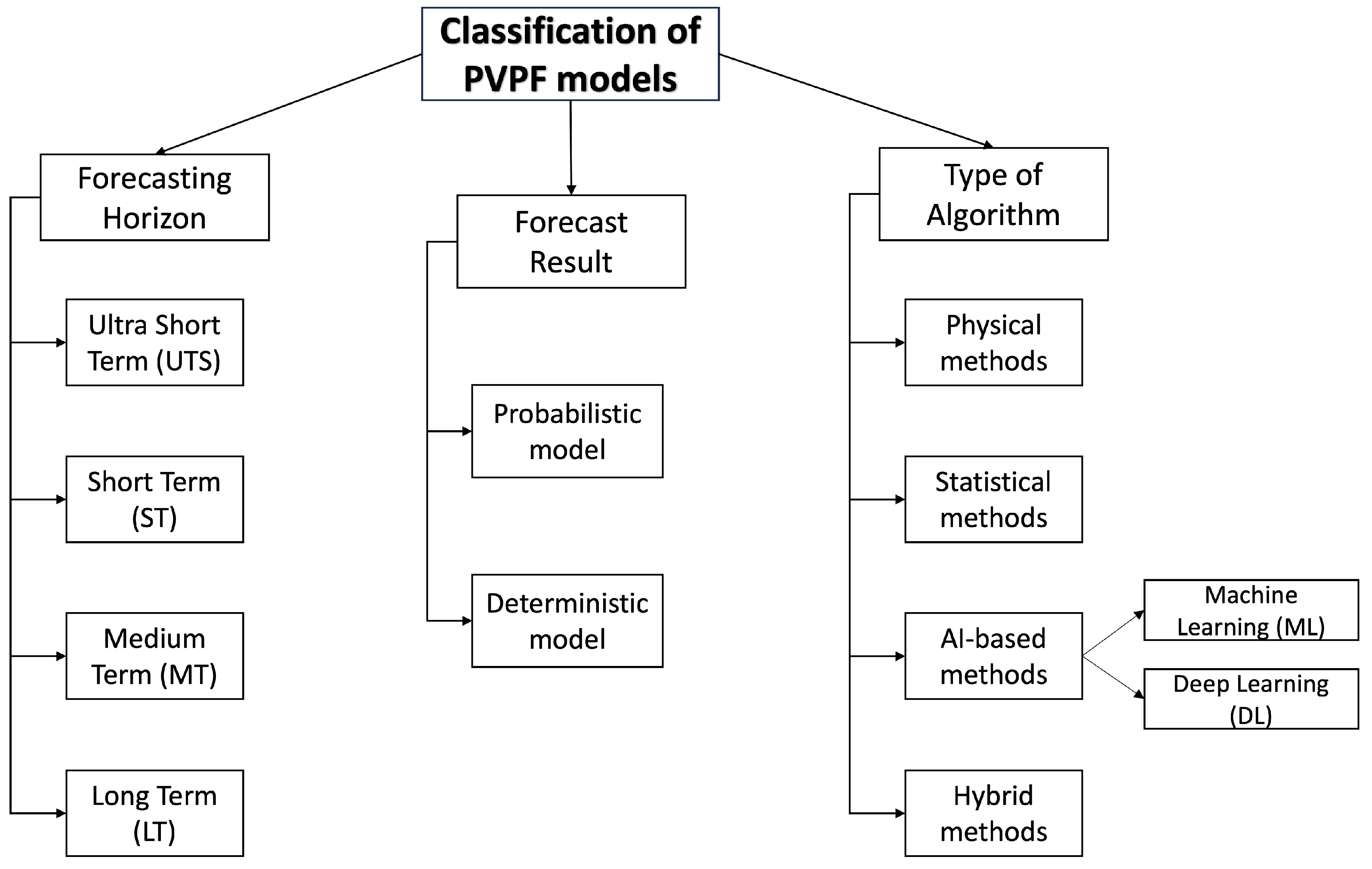
To accurately describe the PV forecasting problem, recent studies [3] can be classified by considering (i) the forecasting horizon, (ii) the forecast result, and (iii) the type of algorithm, as schematically displayed in Figure 1.
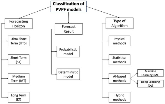
Figure 1.
PVPF classification by: (i) the forecasting horizon, (ii) the forecast result, (iii) the type of algorithm. (Our elaboration).
First, different time horizons were considered for forecasting. The literature [13] classifies PV forecasts into four categories based on the forecast horizon, which is the period to forecast future PV power generation: ultra-short-term (minute scale), short-term (hour scale), medium-term (day scale), and long-term (month scale). Each category has various implications for scheduling PV plants. While long-term and medium-term forecasts are valuable for planning, short-term forecasts are indispensable for developing daily power consumption strategies and ensuring the dependable operation of PV power stations.
Some studies have used meteorological data to calculate solar irradiance and predict the future PV power output based on PV power generation models, which are indirect prediction methods. A recent study [14] comprehensively reviewed the value of solar forecasting in the implementation of PVPF methods. Solar forecasting can be classified into two categories, deterministic and probabilistic, based on their uncertainty representations. Deterministic solar forecasting provides a single irradiance/PV power value for each forecast timestep. By contrast, probabilistic solar forecasting can also include information on the probability of occurrence and forecast distribution [15].
Finally, considering the type of algorithm, the most commonly used methods for implementing the PVPF method are as follows.
- Physical models are deterministic closed-form solutions for PVPF. These models depend on data related to solar irradiance; therefore, historical power-generation data are not required. However, accurate predictions require the use of detailed parameters for the PV plants. In most cases, future solar irradiance is obtained from NWP [16]. Additional data, such as meteorological information including temperature, humidity, wind direction, PV plant capacity, and installation angle, may be used to optimize the results [17]. However, solar irradiance is the most crucial meteorological data and NWP is necessary for its effectiveness. Therefore, nearby weather stations are essential to PV performance models [18].
- Statistical methods, which involve extensive numerical pattern analysis based on statistical forecasting, require the acquisition of a historical dataset. Recently, the literature has demonstrated that statistical methods outperform physical ones [19]. Conventional linear statistical techniques are relatively simple and have a limited number of parameters, but are less capable of fitting complex curves [20]. Statistical techniques rely on historical time series and real-time data to identify patterns, and the forecast accuracy depends on the quality and dimensions of the available data. These methods are less costly than physical methods and are generally better for short-term forecasting. These models are useful tools for predicting linear data, but they are limited to nonlinear data. Consequently, they are often combined with artificial intelligence algorithms to improve accuracy [21].
- The use of artificial intelligence techniques, which incorporate advanced methods for acquiring knowledge and expertise, has led to precise outcomes and enhanced generalization capabilities. These approaches provide greater flexibility through dynamic learning procedures, thereby enabling real-time computation. These methods, including machine learning (ML) and deep learning (DL), offer more complex structures and numerous parameters than the conventional models. DL models can learn from parsed data representations using a general learning process without requiring the user to perform specific feature extraction processes, which distinguishes them from conventional ML models. Efficient DL variants, such as LSTM [22], Bidirectional LSTM (BiLSTM) [23], and Gated Recurrent Units (GRU) [24], have been proven to extract and analyze nonlinear and non-stationary characteristics of time-series data and have been employed to predict renewable energy production.
- Hybrid methods, which combine the previously discussed methods, are also widely considered in the recent literature [25]. HMs aim to produce better outcomes than simple methods but can be more complex and time-consuming to train. Typically, they are effective for short- and long-term forecasting [26]. The data requirements for HMs depend on the models used in the hybrid approach. For instance, if two sub-models require different types of data, HM will require four types of data. HMs can use physical or statistical models as a foundation and then incorporate DL techniques to capture nonlinearities or rectify model biases.
Related Works
In [27], an HM method based on a Convolutional Neural Network (CNN) and LSTM was proposed for the prediction of electric charges, and its performance was compared with that of other models.
The work in [28] introduced a prediction error-based power forecasting method for PV for utility-scale application systems using model-based gray box neural networks, which require less training time than black box neural network-based models. In [29] the authors presented an LSTM system that learns from newly arrived data using a two-phase adaptive learning strategy and a sliding-window algorithm to detect concept drifts in PV systems.
In [30] authors proposed an LSTM attention-embedding model based on BO to predict the day-ahead PV power generation. The model consists of an LSTM block, an embedding block, and an output block. In [31], a model based on a two-stage attention mechanism over LSTM was proposed to forecast day-ahead PV power, with BO applied to obtain the optimal combination of hyperparameters.
A collection of DL techniques, such as LSTM, BiLSTM, GRU, CNN, and HM, was presented in [32]. In this study, the authors conducted a comparative analysis of PVPF methods by utilizing a BO algorithm, which demonstrated the improved performance of the LSTM model compared with other models.
A research paper by [33] introduced a PVPF method integrated with the HW statistical forecasting method using historical PV profile data and a forecasting parameter (alpha). The primary advantages of the proposed method are its simplicity and satisfactory performance for short-term forecasting. Another study [34] proposed a hybrid method based on HW and ML to predict residential electricity consumption at a 15-min resolution, where the HW model was employed to model the stationary component of consumption. With regard to predictive maintenance, the authors of [35] presented an annual assessment of the performance degradation of three PV module technologies using four statistical methods including the HW method.
In [36], the authors proposed a method that combines the multiplicative HW model and a fruit-fly optimization algorithm to determine the optimal smoothing parameters for the exponential smoothing method. The Mean Absolute Percentage Error (MAPE) was used as the evaluation metric, and the results showed that the proposed model significantly improves accuracy, even when limited training data are available.
In [37], a PVPF method based on six time-series algorithms including HW and LSTM was developed for nonstationary data. According to the authors, the main reason for using time-series models is that they apply to PVPF approaches that consider the period, trend, and seasonality.
3. The Proposed Framework
This section outlines the baseline methods considered in our study: the HW triple-exponential smoothing method, which is particularly designed for time-series data; the LSTM method, which is capable of learning long-term dependencies in the data and making accurate predictions based on that information; and the BO method, which is a probabilistic optimization algorithm utilized to discover the optimal set of LSTM hyperparameters.
3.1. Triple Exponential Smoothing
Exponential smoothing methods offer precise forecasts by relying on historical data and by assigning greater importance to recent observations. Specifically, time-series data can be modeled using three components: trend or long-term variation, seasonal components, and irregular or unpredictable components. These components can be combined using either additive or multiplicative procedures.
In the additive model, the series demonstrated consistent cyclic variations, regardless of their level. However, the multiplicative model assumes that the amplitude of seasonal fluctuations changes as the series trend varies. It is important to note that a multiplicative HW model can be transformed into an additive HW model by applying a Box–Cox transformation. This statistical technique is used to modify a dataset so that the transformed data have a more suitable distribution for analysis.
The additive method predicts the values of time series using the following procedure:
At each iteration of index t, the algorithm updates , , and using three equations, each depending on a smoothing parameter with values in the interval , that is, , , and , respectively.
The parameter in the level equation is responsible for smoothing. A lower value of places greater emphasis on the historical data, whereas a higher value assigns more weight to recent observations. Parameter is used to determine the trend estimation and is adjusted based on its proximity to 0 and 1. A value close to zero emphasizes the trend, whereas a value close to one assigns more weight to the observations. The parameter is responsible for controlling the smoothness of the seasonal component and affects the model’s sensitivity to fluctuations in the series. As the value of increases, predictions become more sensitive.
Algorithm 1 describes the additive HW (AHW) method used in the study. The algorithm requires three inputs: seasonal parameter s, forecast time width h, and historical time series of n values, denoted as . The output of the algorithm is , that is, the forecast at the final instant . Therefore, the algorithm produces forecasts based on historical data, estimated trends, and seasonal patterns.
| Algorithm 1 Additive Holt–Winters (AHW) |
|
In our implementation, we employed mean absolute scale error (MASE) as an accuracy measure for the AHW algorithm. This measure is preferred because it is not scale-dependent, does not result in undefined or infinite values, and provides accurate results. The MASE is calculated as , where , is the mean absolute error (MAE), and are the actual and forecast values in period t, respectively, and is the scaling factor, where p is the sampling frequency per day.
Our goal was to identify the ideal smoothing parameters that minimize the error function MASE. To achieve this goal, we used R2023b MATLAB’s built-in optimization tool based on a Genetic Algorithm (GA function ga). This GA implementation is inspired by the principles of biological evolution and genetics in nature, and has strong global search capabilities that make it effective for finding better solutions in large search spaces.
3.2. Long Short-Term Memory
Recurrent neural networks (RNNs) are commonly utilized in deep-learning frameworks owing to their capacity to process sequential data. These networks are composed of interconnected neurons, where the output of one neuron not only influences the next layer, but also feeds back to the previous layer. This arrangement facilitates the retention of the underlying information until it is fed back into the subsequent prediction, making it simpler to implement and train the network. However, RNNs have limited ability to handle long-term dependencies in sequential data, which can result in challenges such as vanishing and exploding gradients. Vanishing gradients occur when gradients during backpropagation significantly diminish, making adequate weight updates challenging, whereas exploding gradients result from large gradients accumulating during backpropagation, leading to unstable models owing to substantial weight updates. Consequently, RNNs have a limited capacity to manage long-term dependencies.
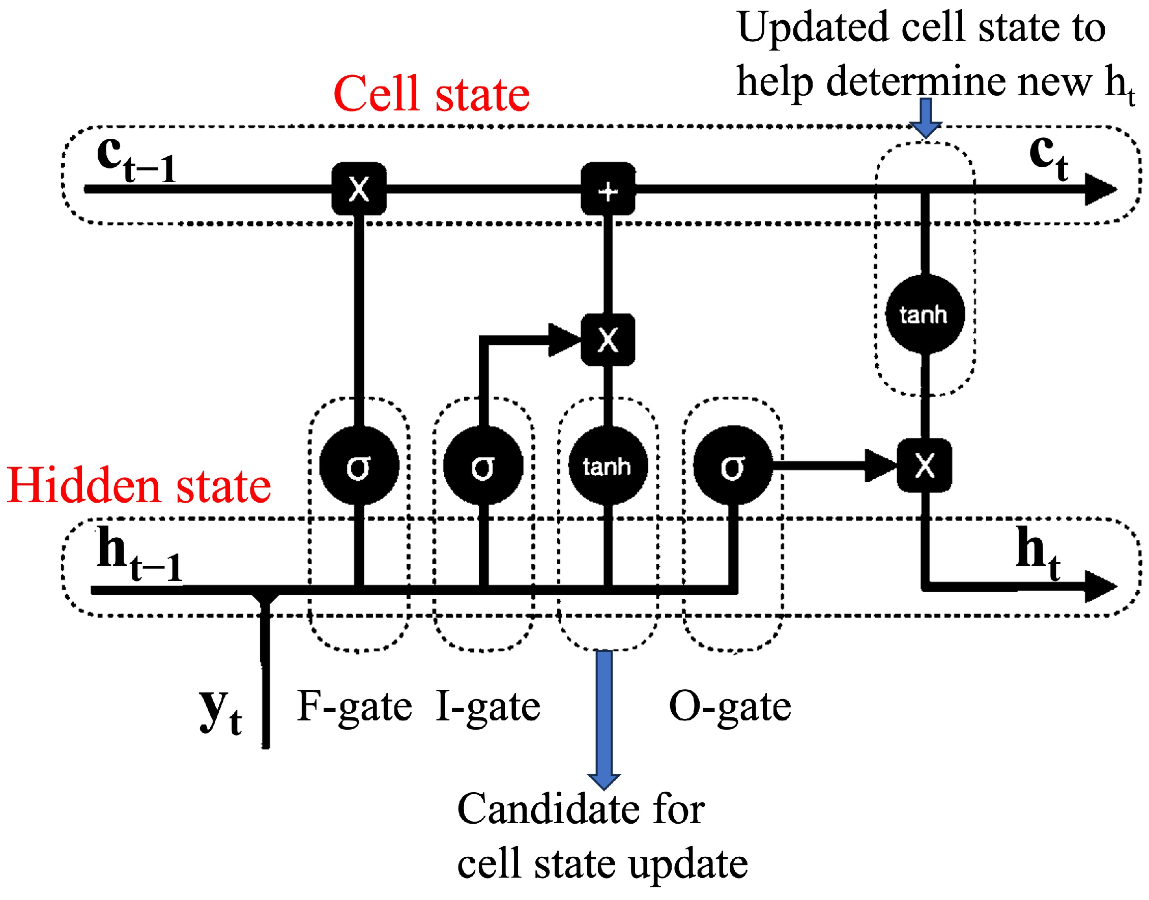
LSTM networks enhance predictions for medium- and long-term data by incorporating additional state and gate control units on top of RNNs. This is facilitated by internal mechanisms that regulate the flow of relevant information in both short and long terms. The fundamental structure of an LSTM cell includes a cell state that preserves long-term memory, and a hidden state that retains short-term memory, as illustrated in Figure 2.

Figure 2.
LSTM cell structure. (Our elaboration).
In Figure 2, three gates are incorporated to regulate the flow of information through the memory cell. The input gate controls the amount of information read into the cell, while the forget gate determines the amount of past information that must be forgotten and retained. The output gate was responsible for reading the output from the cell. This design allows the cell to decide when to retain information and ignore inputs, which is crucial for remembering useful information and forgetting less-useful information.
Mathematically, these gates are computed as follows.
In the previous equations, , and represent the input, forget, and output gates at the current time step t, respectively. The variable represents the input at time t and is the hidden state at the previous time step. W and U represent the weight matrices and b is the bias vector. is the sigmoid activation function that sets the values of these gates in the range .
The memory cell and hidden state are updated as follows.
The candidate memory cell, denoted by , can capture both the previous information stored in and current input value . The calculation of the content of the memory cell, represented by , is determined by the past memory cell state and current memory cell candidate, which functions as the current input. The process of determining the amount of past information to be discarded and the amount of current input to be retained is facilitated by element-wise matrix multiplication represented by ⊙ and an activation function.
In this process, and are used to control the amount of information discarded or retained in the element-wise matrix multiplication. For instance, when the values of are close to zero, the results of the element-wise matrix multiplication between and render past information negligible or, in other words, obsolete. The computation of the hidden state depends on the memory cell and the extent to which the memory cell output is passed as an output is regulated by the output gate .
3.3. Hyperparameter Optimization
DL models are influenced by various factors such as the choice of an appropriate loss function, optimization procedure, and hyperparameters. Hyperparameters are parameters that models cannot learn during the training process but may affect the models’ performance. For RNNs, the number of hidden layers, units in each hidden layer, and the learning rate are important hyperparameters.
The process of identifying the hyperparameter configuration that leads to optimal generalization performance is known as hyperparameter optimization. We utilized the Bayesian optimization (BO) algorithm for this optimization procedure, which is discussed in detail in the next section. In our experiments, the following hyperparameters were optimized: (i) units in the hidden layer, (ii) number of hidden layers, (iii) use of BiLSTM layers, (iv) initial learning rate, and (v) L2 Regularization.
The Adam optimizer was utilized during the training process for the model, and the units in the hidden layer, the number of hidden layers, and the initial learning rate were fine-tuned through an optimization procedure. Moreover, our study included the following two additional hyperparameters to be optimized:
- A flag that modifies the layers in the LSTM model from unidirectional to bidirectional. In the bidirectional case, an LSTM layer assesses the input sequence from both forward and backward directions, and the final output vector is derived from a combination of the final forward and backward outputs.
- The decay factor of the L2 regularization approach. This approach allows the learning process to simultaneously minimize the prediction loss and penalty term introduced into the loss function of the training model. The updated loss function with weight decay is expressed aswhere refers to the root mean square error from the network outputs and represents the trainable parameters of the LSTM, with p being the total number of such parameters. The decay factor is set to a specific value, indicating that the model will strive to minimize the loss while ensuring that the sum of the squares of the LSTM layer’s weights does not exceed times the output of the layer. The regularization term is included in the loss function in each iteration of the training process, and the model is optimized to minimize the total loss, including the regularization term.
L2 regularization is a widely used technique in the field of machine learning to avoid overfitting, particularly in LSTM models. Overfitting occurs when a model becomes excessively complex and learns the noise present in the training data, leading to a poor performance on unseen data. L2 regularization is a straightforward and efficient method for preventing overfitting in LSTM models, and can significantly enhance the performance of the model on new data.
BO is an efficient algorithm for exploring extensive hyperparameter-search spaces. The optimization technique is based on a probabilistic surrogate model to represent the actual objective function, which is then used in conjunction with an acquisition function to guide the search process.
The first step in the BO process is to identify the objective function to be optimized, which can be the loss function or another function deemed appropriate for model selection. The surrogate model, which is less expensive than the actual function, is used as an approximation when evaluating the objective function. BO is a sequential process, because the determination of the next promising points to search depends on the information from the previously searched points. The acquisition function, another critical component of BO, directs the search for potential areas with low objective function values, thereby facilitating a balance between exploitation and exploration.
Constructing a probabilistic surrogate model involves selecting a sample of points through a random search or another method, fitting a probability model to these points, and iteratively updating the model using acquisition and objective functions. This process continued until the termination condition was satisfied. Gaussian processes are a common choice for surrogate models and are characterized by a set of random variables that, when combined, result in a joint Gaussian distribution. In this study, the built-in BO tool (function bayesopt) in MATLAB is used.
4. Materials and Methods
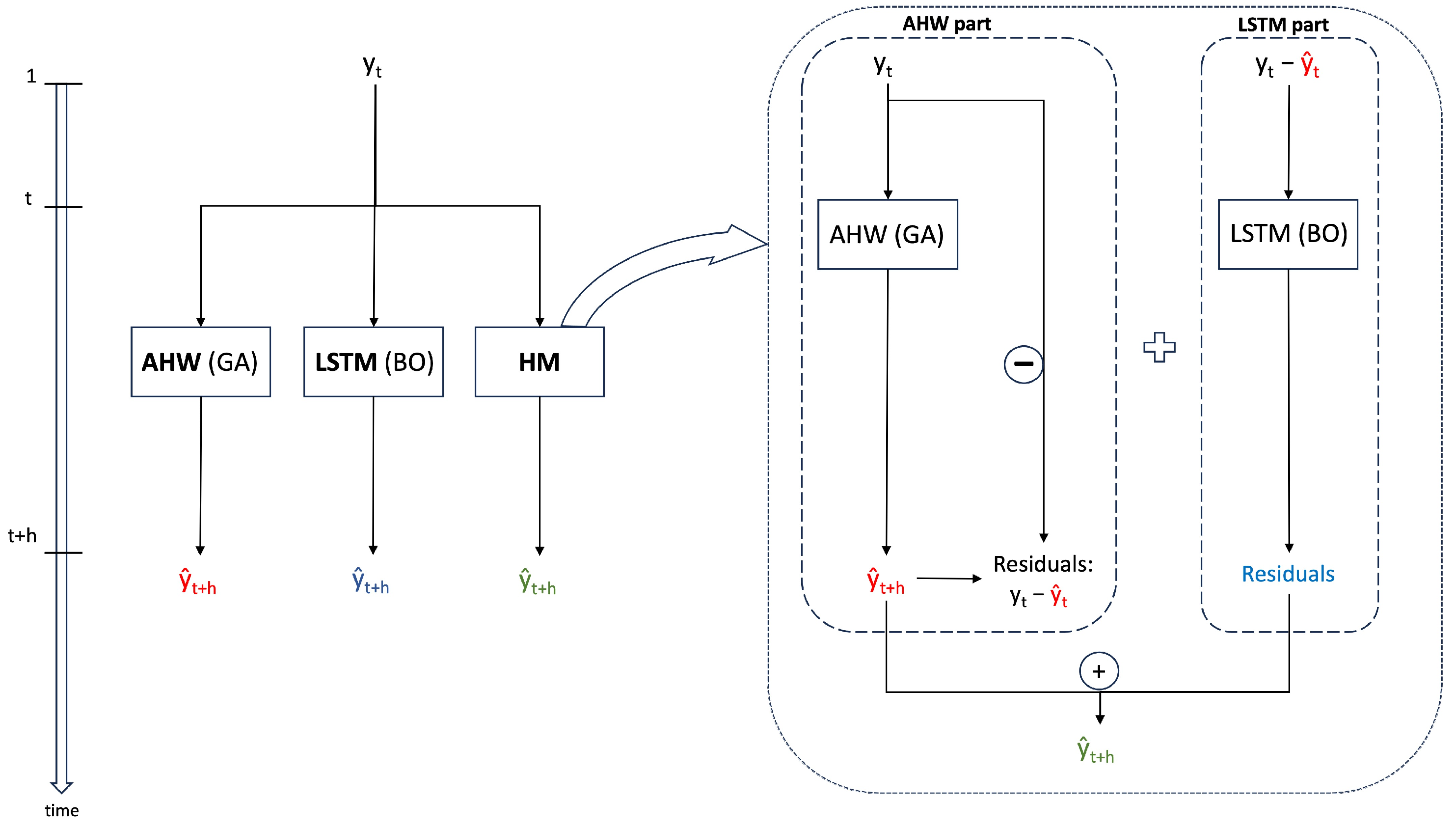
We compared three PVPF methods, namely AHW, LSTM, and HM. The HM method uses AHW to forecast data, followed by computation of a time series of residuals between past forecast AHW data and actual past data (i.e., the forecast error is calculated as the difference between and ). The LSTM component of the HM method is then trained to predict the residual time series. Finally, the predicted value of the HM method was obtained by combining the outputs of AHW and LSTM on the residuals.
To optimize the smoothing parameters of the AHW, we utilized the GA approach. By contrast, we employed the BO algorithm as an auto-configuring approach to determine the optimal LSTM network structure among predefined intervals of hyperparameters, thereby reducing the need for data analyst intervention for each of the three forecasting methods evaluated in our study.
Figure 3 illustrates a schematic overview of the three models examined in our comparative study as well as a flowchart detailing the steps involved in implementing one model over another.
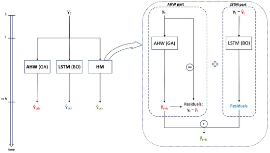
Figure 3.
Representation of the PVPF methods. Red, blue, and green colors are used to represent the forecasts generated by the AHW, LSTM, and HM models, respectively. (Our elaboration).
The approaches receive the historical time series of the PV power output as input, with the forecast computed for h steps ahead of the current time of the index t. Figure 3, red, blue, and green colors are used to represent forecasts generated by the AHW, LSTM, and HM models, respectively.
The HM model is detailed in the box on the right-hand side of Figure 3. Specifically, the AHW approach was employed to predict the PV power output. Using the historical PV data, the forecasted values produced by the AHW approach were used to generate a time series of residuals. This time series is then utilized to train the LSTM approach, which provides a forecast of the residuals between the AHW and actual PV power output. Finally, the actual forecast computed for h steps ahead in the HM approach was obtained by summing the forecasts of the AHW and residual using the LSTM approach.
4.1. Forecast Accuracy Measures
In this section, we introduce the metrics used to evaluate the forecast accuracy of the models under study, enabling a comparison of their performance. We denote the observation at time t by and the forecast of that observation by . The forecast error is calculated as the difference between and . Let m denote the total forecasted period.
The root mean square error (RMSE) is the most commonly used scale-dependent measure. We used the normalized RMSE (nRMSE), which measures the variability in errors and is often expressed as a percentage, where lower values indicate a lower residual variance. Although there are no consistent means of normalization in the literature, we considered the mean of the measurement to normalize the RMSE. nRMSE measures the difference between the predicted values and the actual values, and is a useful metric for evaluating the accuracy of the model.
To comprehensively assess the relationship between total and pairwise errors, we also measured pairwise total errors. This was achieved by computing the correlation between the ranks of these errors. To provide a more robust indicator of extreme values, we consider the rank of the errors rather than the errors themselves. To calculate Spearman’s rank correlation coefficient, we employed the following method:
where is the distance between the ranks of time series and . Similar to the other correlation coefficients, the values of the Spearman’s rank correlation varied between and 1. A strong positive correlation, that is, a distance rank score close to 1, suggests high performance in forecasting. The Spearman’s rank correlation is a measure of the strength of the relationship between two variables, based on their rankings rather than their actual values. It is particularly useful in situations where the data may be skewed or contain outliers.
The R2 coefficient of determination measures how well the model predicts an outcome, or the proportion of variation in the observed dataset predicted by the forecasting method. The lowest possible value of R2 was zero, whereas the highest possible value was one. The R2 measures the proportion of variance in the actual values that is explained by the model, and can be used to evaluate the model’s predictive performance. It is defined as follows.
4.2. Case Study
The case study used PV power-generation data obtained from a publicly accessible database maintained by the National Institute of Standards and Technology [38]. This database provides historical PV power generation data for two PV power plants that are located in close proximity. This dataset has been widely utilized in recent studies [39,40,41] and is divided into two subsets: D1 contains data for a larger farm with a rated power of 243 kW, and D2 contains data for a smaller farm with a rated power of 75 kW.
In our study, we utilized dataset D2, with reference to the output power of inverter no. 2, measured in watts (W) during the second year of observations, as a numerical case study. We focused on the hourly generated power to reduce the data density. Days with missing values were filled with zero production values to maintain the integrity of the time-series. The original data provided timestamps and 24 h power production data for each day. Neither meteorological features nor NWP data were considered.
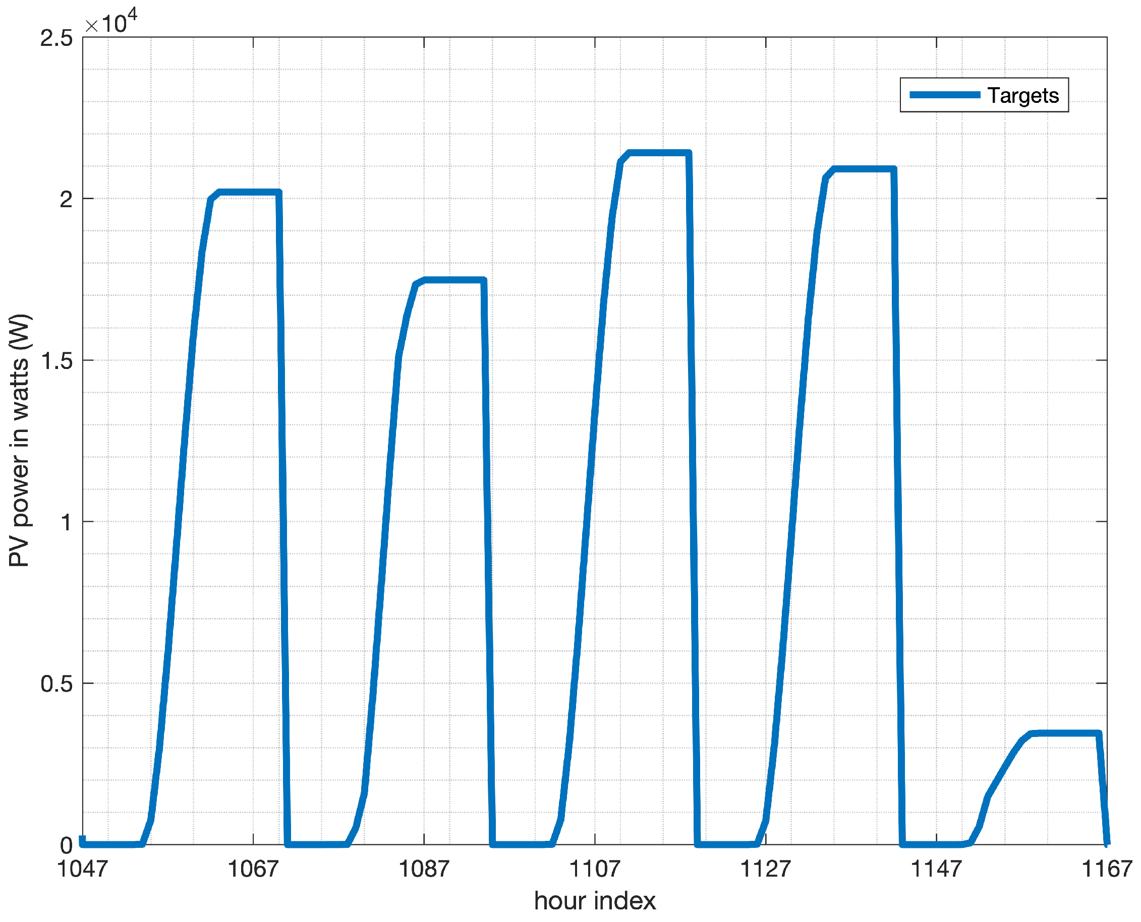
The primary objective of this case study is to investigate the daily PV power generation, which exhibits diverse output shapes each day, as depicted in Figure 4. This figure shows a random row of five consecutive days from the dataset, and illustrates that the output patterns vary across different days. Daily PV power generation exhibits cyclic behavior during daytime hours and may have different peak values depending on weather conditions. Sunny days ensure maximum PV power generation capacity. In contrast, rainy or cloudy days may produce less or negligible power from the PV plants.

Figure 4.
PV power outputs in in watts (W vertical y-axis) in a row of five days corresponding to 120 hourly observations ranging from hour no. 1047 to hour no. 1167 (horizontal x-axis).
Table 1 presents the hyperparameters to be optimized in the proposed LSTM model, including the number of units in the embedding and LSTM layers. A BO algorithm was employed to optimize the five parameters of the proposed LSTM model, as described in Section 3.3. The optimal set of values for these parameters along with the convergence time of the optimization algorithm are listed in Table 2.

Table 1.
Hyperparameter, corresponding label for the LSTM method, and definition sets.
Table 2.
Optimal hyperparameters values of three PVPF methods (AHW, LSTM, and HM). The GA was implemented in case of AHW and BO algorithm in the case of LSTM and HM.
Table 2 presents the values for , , and of the AHW method, which were obtained by applying the GA optimization to the error function MASE, as described in Section 3.1. The seasonal component of the AHW method was set equal to the value of , which corresponded to the cyclic fluctuations of PV power generation related to the cyclic behavior of alternating night and day times within the 24-h sampled for each day. As shown in Table 2, the GA optimization of the AHW method achieved the lowest configuration time, whereas the LSTM and HM methods presented higher configuration times, owing to the application of the BO algorithm.
5. Experimental Results and Discussion
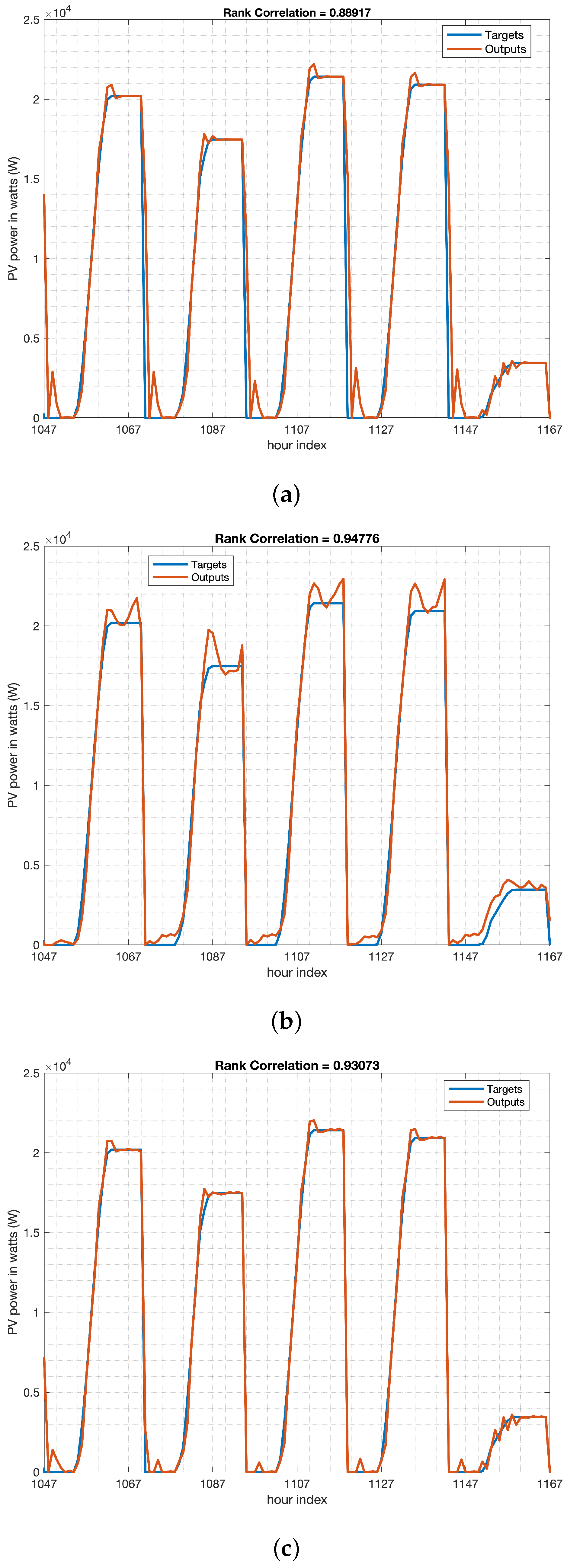
The three PVPF methods were implemented using MATLAB on a computer equipped with an Intel CoreTM i7-6 core processor and 16GB RAM. The results are shown in Figure 5, which presents time-series plots for the testing datasets of the three models, focusing on the period from 3 January 2016, from 00:00 to 8 January 2016, at 00:00, covering 120 hourly observations, ranging from observation no. 1047 to 1167.
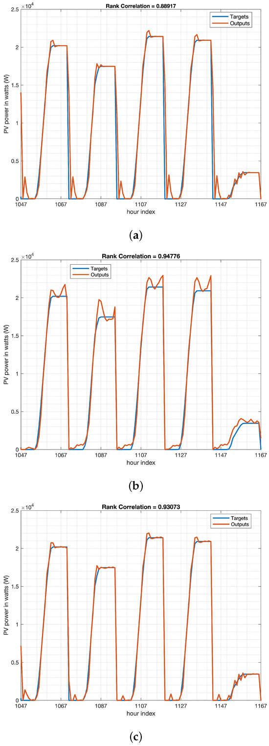
Figure 5.
Examples of PV power forecasting in watts (W vertical y-axis) in a row of five days, with 120 hourly observations ranging from hour no. 1047 to hour no. 1167 (horizontal x-axis). Real observed values labeled as “Targets” (blue line). Predicted data labeled as “Outputs” (orange line). Three techniques: (a) AHW, (b) LSTM, and (c) HM.
The values of, nRMSE, RankCorr, and R2 for the AHW, LSTM, and HM methods are summarized in Table 3 for different training/test data ratios. Notably, both the LSTM and HM models outperformed the AHW model in terms of predicting the PV power output data regardless of the ratio of training to testing data. One of the main reasons why LSTM outperforms the AHW approach is that it can capture long-term dependencies in the data more effectively.
Table 3.
Comparison of the performance of three PVPF methods (AHW, LSTM, and HM) across various train/test splits of the original dataset. Evaluation based on nRMSE, RankCorr, and R2.
The HM method, obtained by combining AHW and LSTM in forecasting PV power generation, can outperform approach compared to each approach alone. This is because the AHW and LSTM are forecasting methods that can complement each other. The AHW is useful for modeling time-series data with a strong seasonal component. It can capture underlying patterns and trends in the data and provide accurate forecasts. However, it may not be effective for capturing short-term fluctuations in data. By contrast, LSTM is effective for learning and modeling complex relationships between variables and making accurate predictions based on the patterns they have learned. However, LSTM may not be as effective as AHW in capturing seasonal patterns in data.
According to recent research, it is possible to compare our methods with those presented in previous studies. Specifically, [39] analyzed six techniques for predicting PV production using the same case study employed in our study. The authors in [39] concluded that CNN is one of the most suitable models for predicting PV production, as it achieved an R2 value of 0.98 in the same case study. From Table 3, it can be observed that our proposed HM technique achieves an R2 value greater than 0.99 on the training dataset, and approximately equal to 0.98 or greater than 0.98 on the testing dataset. Consequently, it can be inferred that the proposed HM technique produces results that are either equivalent or superior to those of other approaches, including the outperforming approach reported in the literature [39]. Notably, our results pertain to the most challenging scenario, which involves generating forecasts during both the daytime and nighttime, as addressed in [39].
By combining the AHW and LSTM methods, we could capture both seasonal patterns and short-term fluctuations in the data. The AHW model can provide a baseline forecast for the data, whereas LSTM can refine the forecast by capturing the complex relationships between the variables. Examples of actual PV power forecasting in watts for the three models in a row of five days are depicted in Figure 5.
Figure 5c highlights that HM effectively leverages the strengths of both the AHW and LSTM models, enabling it to forecast PV power spikes, as the LSTM model alone does in Figure 5b but with smoother results owing to the contributions of the AHW model in Figure 5a, which leads to superior forecasting accuracy.
The LSTM method tends to overestimate the actual data because of its rapid response to fluctuations, often forecasting spikes in power even in the absence of actual peaks (as illustrated in Figure 5b). However, the AHW model exhibits higher inertia, which helps prevent overestimation and results in smoother peaks (as depicted in Figure 5a). As expected, the HM model strikes a balance between the two models by combining their respective advantages (as shown in Figure 5c).
The plots in Figure 6 illustrates the correlation between the actual and predicted PV power for all methods using an 80% training dataset and a 20% testing dataset for the entire validation period. Figure 6 The results suggested a significant linear relationship between these variables. Although the AHW, LSTM, and HM methods yielded similar results, the HM method demonstrated an improved performance because the predicted values were closer to the actual values.
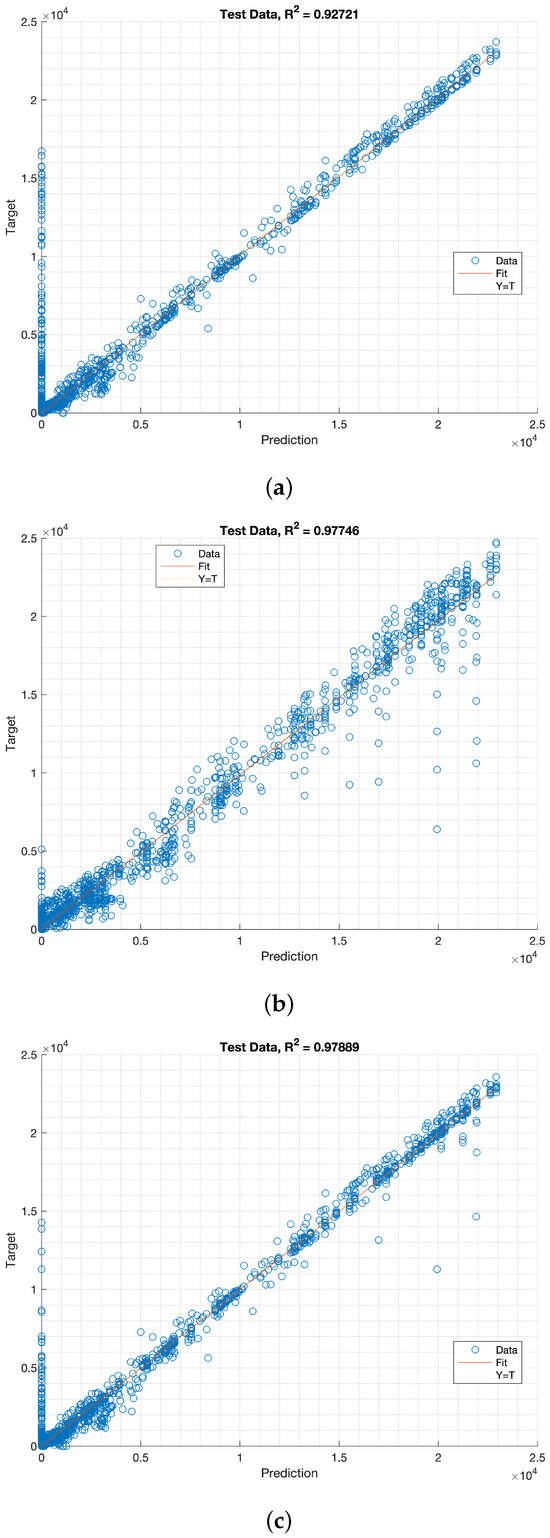
Figure 6.
Scatter graph of the actual and predicted PV power in watts (W) along with the regression lines. Target values on the vertical y-axis. Prediction values on the horizontal x-axis. The test data consisted of 73 days and 1752 hourly predictions. Three techniques: (a) AHW, (b) LSTM, and (c) HM.
The AHW and HM methods exhibit higher latencies than the LSTM model. This was confirmed by the large sample of non-null observations predicted with a zero value (i.e., points on the y-axis) in Figure 6a,c. In contrast, the LSTM model demonstrates higher reactivity, which often results in overestimation of the target values, as seen in the out-of-bound predictions in the range of 20–25 kW and 10–20 kW in Figure 6b.
The discrepancies between the predicted and actual values in the ranges–15–25 kW and 5–20 kW are shown in Figure 6b. Additionally, Figure 6c reveals that the AHW and HMs models exhibit fewer deviations from the fit line, which in turn leads to less overestimation. Conversely, the LSTM model exhibited more pronounced overestimations, as shown in Figure 6c. Regression Plots in Figure 6 illustrates that the AHW and HMs models displayed higher error rates, whereas the LSTM model tended to overshoot the target values.
The AHW method is a simple and efficient approach that has been shown to functions effectively as a PVPF method. However, it has been observed that this method may sometimes underestimate data. In contrast, the LSTM approach is a more complex method that can capture intricate patterns in the PV power data. However, this method is prone to overestimating data.
To address the limitations of both the methods, a hybrid approach was employed. This can help produce more accurate forecasts by mitigating the limitations of each approach. The AHW method provides a baseline forecast, whereas the LSTM model enhances and refines the forecast by considering the intricate data patterns. Our study demonstrates that this refinement can be achieved by training the LSTM model on the residuals between AHW predictions and observed data. By integrating different approaches and using a hybrid model, better results can be achieved, and forecast accuracy can be enhanced.
6. Conclusions
The main objective is to employ forecasting techniques that can effectively address the uncertainty of the PV power fluctuations. These methods can predict the power output of a PV system over a specific period with a certain level of accuracy, which can help manage the associated uncertainties. In our research, we utilized a combination of forecasting techniques, including machine-learning algorithms and statistical models, to enhance the precision of the predictions.
In particular, we investigated the potential advantages of combining AHW with LSTM and BO algorithms within an HM framework for time-series forecasting. AHW is a seasonal decomposition method that can be employed to model and forecast time-series data. LSTM is an RNN that is particularly suitable for processing long-term dependencies in sequential data. BO is an optimization algorithm that utilizes probabilistic models to explore the search space efficiently and identify the optimal solution.
The experimental results showed that by combining these three techniques, it may be possible to enhance the accuracy and efficiency of time-series data forecasting. LSTM can be used to capture long-term dependencies in the data, whereas the AHW algorithm can be used to model and forecast seasonal patterns.
The proposed model does not require substantial computational resources or specialized expertise for implementation and fine-tuning. In the reference case study, the configuration times were not greater than 24 min of computation on a 6-core processor with 16 GB of RAM (i.e., a typical laptop) to be implemented and fine-tuned. Furthermore, no expertise is required from the analyst because the GA and BO algorithms are used to automatically fine-tune the parameters of AHW and LSTM to achieve superior results. Therefore, this approach is suitable for small operations or regions with a limited computational infrastructure.
Through our analysis, we found that integrating statistical modeling with the LSTM and BO algorithms led to more accurate forecasting results compared with using each method alone. These findings imply that the integration of statistical modeling with LSTM and BO algorithms can improve the accuracy and reliability of time-series forecasting of PV energy production. By combining these methods, we can develop more precise and reliable forecasting models that can inform decision making and resource management in this field.
Our research has implications for forecasting PV power data when only historical data of PV power generation are available and NWP data are inaccessible. The proposed methodology can be applied to various geographic locations, climates, and types of renewable energy sources, without limitations. To enhance the current approach, future research could investigate its effectiveness for other renewable energy sources such as wind or hydropower by broadening the scope of this study. Additionally, other time-series models, such as the exponential smoothing state-space model or the seasonal decomposition of the time-series model, can be explored when integrated with the LSTM and BO algorithms. Finally, investigating the impact of data quality, such as missing data, noisy data, or data with outliers, on the effectiveness of the proposed methodology can provide valuable insights.
Finally, it is important to note that the techniques explored in this study rely heavily on the availability of large historical datasets to capture patterns effectively, learn representations, and make accurate discoveries. Therefore, ensuring access to such datasets is essential for successful application of these techniques.
In regions where there is a lack of historical data or when estimating outputs for new installations, it is recommended to utilize physical models that offer deterministic closed-form solutions for the PVPF. However, these models rely on data related to solar irradiance and require detailed parameters for PV plants and expert analyses. To optimize the results, additional data, such as meteorological information including temperature, humidity, wind direction, PV plant capacity, and installation angle, may be considered. When historical datasets are accessible, the cost-effective and computationally efficient techniques explored in this study can be applied, which require minimal expertise for implementation and fine-tuning. In contrast to physical models, these methods do not require substantial resources or specialized knowledge.
Author Contributions
Conceptualization, M.P.; methodology, M.P.; validation, M.P. and A.P.; resources, G.P.; writing—original draft preparation, M.P. and A.P.; writing—review and editing, M.P. and A.P.; supervision, M.P and G.P.; project administration, M.P. and G.P.; funding acquisition, G.P. All authors have read and agreed to the published version of the manuscript.
Funding
This research received no external funding.
Institutional Review Board Statement
Not applicable.
Informed Consent Statement
Not applicable.
Data Availability Statement
The data analyzed in this manuscript are available at https://pages.nist.gov/netzero/data.html (accessed on 9 April 2024).
Acknowledgments
The authors acknowledge the administrative and technical support provided by Advantech S.r.l. industry, Lecce, Italy.
Conflicts of Interest
The authors declare no conflicts of interest.
Abbreviations
The following abbreviations are used in this manuscript:
| AHW | Additive Holt–Winters |
| BiLSTM | Bidirectional Long Short-Term Memory |
| BO | Bayesian Optimization |
| CNN | Convolutional Neural Network |
| DL | Deep Learning |
| HM | Hybrid Model |
| HW | Holt–Winters |
| LSTM | Long Short-Term Memory |
| MAE | Mean Absolute Error |
| MAPE | Mean Absolute Percentage Error |
| MASE | Mean Absolute Scaled Error |
| ML | Machine Learning |
| nRMSE | normalized Root Mean Square Error |
| PV | Photovoltaic |
| PVPF | Photovoltaic Power Forecasting |
| RankCorr | Spearman’s Rank Correlation coefficient |
| RMSE | Root Mean Square Error |
| RNNs | Recurrent Neural Networks |
References
- Hao, F.; Shao, W. What really drives the deployment of renewable energy? A global assessment of 118 countries. Energy Res. Soc. Sci. 2021, 72, 101880. [Google Scholar] [CrossRef]
- Wang, J.; Azam, W. Natural resource scarcity, fossil fuel energy consumption, and total greenhouse gas emissions in top emitting countries. Geosci. Front. 2024, 15, 101757. [Google Scholar] [CrossRef]
- Abdulla, H.; Sleptchenko, A.; Nayfeh, A. Photovoltaic systems operation and maintenance: A review and future directions. Renew. Sustain. Energy Rev. 2024, 195, 114342. [Google Scholar] [CrossRef]
- Wang, Q.; Paynabar, K.; Pacella, M. Online automatic anomaly detection for photovoltaic systems using thermography imaging and low rank matrix decomposition. J. Qual. Technol. 2022, 54, 503–516. [Google Scholar] [CrossRef]
- Mellit, A.; Massi Pavan, A.; Ogliari, E.; Leva, S.; Lughi, V. Advanced methods for photovoltaic output power forecasting: A review. Appl. Sci. 2020, 10, 487. [Google Scholar] [CrossRef]
- Mohapatra, B.; Sahu, B.K.; Pati, S.; Bajaj, M.; Blazek, V.; Prokop, L.; Misak, S. Optimizing grid-connected PV systems with novel super-twisting sliding mode controllers for real-time power management. Sci. Rep. 2024, 14, 4646. [Google Scholar] [CrossRef]
- Brotzge, J.A.; Berchoff, D.; Carlis, D.L.; Carr, F.H.; Carr, R.H.; Gerth, J.J.; Gross, B.D.; Hamill, T.M.; Haupt, S.E.; Jacobs, N.; et al. Challenges and opportunities in numerical weather prediction. Bull. Am. Meteorol. Soc. 2023, 104, E698–E705. [Google Scholar] [CrossRef]
- Xia, P.; Min, M.; Yu, Y.; Wang, Y.; Zhang, L. Developing a near real-time cloud cover retrieval algorithm using geostationary satellite observations for photovoltaic plants. Remote Sens. 2023, 15, 1141. [Google Scholar] [CrossRef]
- Chen, Z.; Amani, A.M.; Yu, X.; Jalili, M. Control and optimisation of power grids using smart meter data: A review. Sensors 2023, 23, 2118. [Google Scholar] [CrossRef]
- Mohamad Radzi, P.N.L.; Akhter, M.N.; Mekhilef, S.; Mohamed Shah, N. Review on the application of photovoltaic forecasting using machine learning for very short-to long-term forecasting. Sustainability 2023, 15, 2942. [Google Scholar] [CrossRef]
- Ren, W.; Jin, N.; Ouyang, L. Phase Space Graph Convolutional Network for Chaotic Time Series Learning. IEEE Trans. Ind. Inform. 2024, 1–9. [Google Scholar] [CrossRef]
- Ahmed, S.F.; Alam, M.S.B.; Hassan, M.; Rozbu, M.R.; Ishtiak, T.; Rafa, N.; Mofijur, M.; Shawkat Ali, A.; Gandomi, A.H. Deep learning modelling techniques: Current progress, applications, advantages, and challenges. Artif. Intell. Rev. 2023, 56, 13521–13617. [Google Scholar] [CrossRef]
- Raza, M.Q.; Nadarajah, M.; Ekanayake, C. On recent advances in PV output power forecast. Sol. Energy 2016, 136, 125–144. [Google Scholar] [CrossRef]
- Gandhi, O.; Zhang, W.; Kumar, D.S.; Rodríguez-Gallegos, C.D.; Yagli, G.M.; Yang, D.; Reindl, T.; Srinivasan, D. The value of solar forecasts and the cost of their errors: A review. Renew. Sustain. Energy Rev. 2024, 189, 113915. [Google Scholar] [CrossRef]
- Yang, D.; Kleissl, J.; Gueymard, C.A.; Pedro, H.T.; Coimbra, C.F. History and trends in solar irradiance and PV power forecasting: A preliminary assessment and review using text mining. Sol. Energy 2018, 168, 60–101. [Google Scholar] [CrossRef]
- Mayer, M.J.; Yang, D.; Szintai, B. Comparing global and regional downscaled NWP models for irradiance and photovoltaic power forecasting: ECMWF versus AROME. Appl. Energy 2023, 352, 121958. [Google Scholar] [CrossRef]
- Delgado, C.J.; Alfaro-Mejía, E.; Manian, V.; O’Neill-Carrillo, E.; Andrade, F. Photovoltaic Power Generation Forecasting with Hidden Markov Model and Long Short-Term Memory in MISO and SISO Configurations. Energies 2024, 17, 668. [Google Scholar] [CrossRef]
- Benavides Cesar, L.; Amaro e Silva, R.; Manso Callejo, M.Á.; Cira, C.I. Review on spatio-temporal solar forecasting methods driven by in situ measurements or their combination with satellite and numerical weather prediction (NWP) estimates. Energies 2022, 15, 4341. [Google Scholar] [CrossRef]
- Massidda, L.; Bettio, F.; Marrocu, M. Probabilistic day-ahead prediction of PV generation. A comparative analysis of forecasting methodologies and of the factors influencing accuracy. Sol. Energy 2024, 271, 112422. [Google Scholar] [CrossRef]
- Chodakowska, E.; Nazarko, J.; Nazarko, Ł.; Rabayah, H.S.; Abendeh, R.M.; Alawneh, R. Arima models in solar radiation forecasting in different geographic locations. Energies 2023, 16, 5029. [Google Scholar] [CrossRef]
- Chen, Y.; Bhutta, M.S.; Abubakar, M.; Xiao, D.; Almasoudi, F.M.; Naeem, H.; Faheem, M. Evaluation of machine learning models for smart grid parameters: Performance analysis of ARIMA and Bi-LSTM. Sustainability 2023, 15, 8555. [Google Scholar] [CrossRef]
- Chen, B.; Lin, P.; Lai, Y.; Cheng, S.; Chen, Z.; Wu, L. Very-short-term power prediction for PV power plants using a simple and effective RCC-LSTM model based on short term multivariate historical datasets. Electronics 2020, 9, 289. [Google Scholar] [CrossRef]
- Herrera-Casanova, R.; Conde, A.; Santos-Pérez, C. Hour-Ahead Photovoltaic Power Prediction Combining BiLSTM and Bayesian Optimization Algorithm, with Bootstrap Resampling for Interval Predictions. Sensors 2024, 24, 882. [Google Scholar] [CrossRef] [PubMed]
- Mahjoub, S.; Chrifi-Alaoui, L.; Marhic, B.; Delahoche, L. Predicting energy consumption using LSTM, multi-layer GRU and drop-GRU neural networks. Sensors 2022, 22, 4062. [Google Scholar] [CrossRef]
- Huang, Y.; Zhou, M.; Yang, X. Ultra-short-term photovoltaic power forecasting of multifeature based on hybrid deep learning. Int. J. Energy Res. 2022, 46, 1370–1386. [Google Scholar] [CrossRef]
- Li, P.; Zhou, K.; Lu, X.; Yang, S. A hybrid deep learning model for short-term PV power forecasting. Appl. Energy 2020, 259, 114216. [Google Scholar] [CrossRef]
- Rafi, S.H.; Deeba, S.R.; Hossain, E. A short-term load forecasting method using integrated CNN and LSTM network. IEEE Access 2021, 9, 32436–32448. [Google Scholar] [CrossRef]
- Shah, A.A.; Ahmed, K.; Han, X.; Saleem, A. A novel prediction error-based power forecasting scheme for real pv system using pvusa model: A grey box-based neural network approach. IEEE Access 2021, 9, 87196–87206. [Google Scholar] [CrossRef]
- Luo, X.; Zhang, D. An adaptive deep learning framework for day-ahead forecasting of photovoltaic power generation. Sustain. Energy Technol. Assess. 2022, 52, 102326. [Google Scholar] [CrossRef]
- Yang, T.; Li, B.; Xun, Q. LSTM-attention-embedding model-based day-ahead prediction of photovoltaic power output using Bayesian optimization. IEEE Access 2019, 7, 171471–171484. [Google Scholar] [CrossRef]
- Aslam, M.; Lee, S.J.; Khang, S.H.; Hong, S. Two-stage attention over LSTM with Bayesian optimization for day-ahead solar power forecasting. IEEE Access 2021, 9, 107387–107398. [Google Scholar] [CrossRef]
- Guanoluisa, R.; Arcos-Aviles, D.; Flores-Calero, M.; Martinez, W.; Guinjoan, F. Photovoltaic Power Forecast Using Deep Learning Techniques with Hyperparameters Based on Bayesian Optimization: A Case Study in the Galapagos Islands. Sustainability 2023, 15, 12151. [Google Scholar] [CrossRef]
- Kanchana, W.; Sirisukprasert, S. PV Power Forecasting with Holt–Winters Method. In Proceedings of the 2020 8th International Electrical Engineering Congress (iEECON), Chiang Mai, Thailand, 4–6 March 2020; pp. 1–4. Available online: https://pages.nist.gov/netzero/data.html (accessed on 9 April 2024).
- Liu, C.; Sun, B.; Zhang, C.; Li, F. A hybrid prediction model for residential electricity consumption using holt-winters and extreme learning machine. Appl. Energy 2020, 275, 115383. [Google Scholar] [CrossRef]
- Adar, M.; Najih, Y.; Chebak, A.; Mabrouki, M.; Bennouna, A. Performance degradation assessment of the three silicon PV technologies. Prog. Photovolt. Res. Appl. 2022, 30, 1149–1165. [Google Scholar] [CrossRef]
- Jiang, W.; Wu, X.; Gong, Y.; Yu, W.; Zhong, X. Monthly electricity consumption forecasting by the fruit fly optimization algorithm enhanced Holt–Winters smoothing method. arXiv 2019, arXiv:1908.06836. [Google Scholar]
- Kim, E.; Akhtar, M.S.; Yang, O.B. Designing solar power generation output forecasting methods using time series algorithms. Electr. Power Syst. Res. 2023, 216, 109073. [Google Scholar] [CrossRef]
- Hunter Fanney, A.; Healy, W.; Payne, V.; Kneifel, J.; Ng, L.; Dougherty, B.; Ullah, T.; Omar, F. Small changes yield large results at NIST’s Net-zero energy residential test facility. J. Sol. Energy Eng. 2017, 139, 061009. [Google Scholar] [CrossRef]
- Cordeiro-Costas, M.; Villanueva, D.; Eguía-Oller, P.; Granada-Álvarez, E. Machine learning and deep learning models applied to photovoltaic production forecasting. Appl. Sci. 2022, 12, 8769. [Google Scholar] [CrossRef]
- Cordeiro-Costas, M.; Villanueva, D.; Eguía-Oller, P.; Martínez-Comesaña, M.; Ramos, S. Load forecasting with machine learning and deep learning methods. Appl. Sci. 2023, 13, 7933. [Google Scholar] [CrossRef]
- Miraftabzadeh, S.M.; Longo, M.; Brenna, M. Knowledge Extraction from PV Power Generation with Deep Learning Autoencoder and Clustering-Based Algorithms. IEEE Access 2023, 11, 69227–69240. [Google Scholar] [CrossRef]

Disclaimer/Publisher’s Note: The statements, opinions and data contained in all publications are solely those of the individual author(s) and contributor(s) and not of MDPI and/or the editor(s). MDPI and/or the editor(s) disclaim responsibility for any injury to people or property resulting from any ideas, methods, instructions or products referred to in the content. |
© 2024 by the authors. Licensee MDPI, Basel, Switzerland. This article is an open access article distributed under the terms and conditions of the Creative Commons Attribution (CC BY) license (https://creativecommons.org/licenses/by/4.0/).