PadGAN: An End-to-End dMRI Data Augmentation Method for Macaque Brain

Abstract

Currently, an increasing number of macaque brain MRI datasets are being made publicly accessible. Unlike human, publicly accessible macaque brain datasets suffer from data quality in diffusion magnetic resonance imaging (dMRI) data. Typically, dMRI data require a minimum ratio of 1:10 between low b-value (b < 10) volumes and high b-value (b > 300) volumes. However, the currently accessible macaque datasets do not meet this ratio. Due to site differences in macaque brain images, traditional human brain image-to-image translation models struggle to perform well on macaque brain images. Our work introduces a novel end-to-end primary-auxiliary dual generative adversarial network (PadGAN) for generating low b-value images. The auxiliary generator in the PadGAN is responsible for extracting the latent space features from peak information maps and transmitting them to the primary generator, enabling the primary generator to generate images with rich details. Experimental results demonstrate that PadGAN outperforms existing methods both qualitatively and quantitatively (mean SSIM increased by 0.1139). Diffusion probabilistic tractography using dMRI data augmented by our method yields superior results.

1. Introduction

Studying the macaque brain provides a crucial avenue for understanding human brain mechanisms in neuroscience research [1]. Currently, the macaque monkey serves as a prominent primate model and has become a vital subject for investigating the human brain using various medical imaging techniques [2,3].

Diffusion magnetic resonance imaging (dMRI) technology detects the movement direction of water molecules in the brain, utilizing the anisotropic diffusion characteristics of water molecules in the white matter to reconstruct the white matter in the brain. The b-value represents the intensity of the diffusion-sensitive gradient field, which, along with its corresponding three b-vectors, reflects the influence of microstructural tissue on water diffusion within living tissue in dMRI. Researchers commonly refer to the images corresponding to different b-value intensities in the dMRI volume as b-value images. Diffusion tensor imaging (DTI) estimation and probabilistic tractography techniques are established methods for reconstructing major white matter fiber bundles in brain imaging [4]. Typically, dMRI images consist of multiple b-value images, with low b-value (b < 10, recommend b = 0) volumes serving as the basis for DTI, which is crucial for data analysis in neuroscience research. Nowadays, to mitigate interference such as head motion during acquisition, one low b-value image often corresponds to 5–10 high b-value (b > 300,commonly b = 1000) volumes [5]. However, in some publicly accessible macaque brain dMRI datasets, the ratio of low b-value to high b-value volumes may be below 1:5 or even 1:10, which could be due to the use of early acquisition protocol configurations [6]. The reliability of computed results, such as DTI estimation, from analyses using data that do not meet the required ratio needs further confirmation. Therefore, it is necessary to generate and optimize low b-value volumes in macaque brain dMRI data.

Medical image-to-image translation refers to the method of translation images from an input image modality to an output modality through a mapping relationship. This approach can be used to acquire additional data or complete missing data [7], and it can be applied to downstream tasks in medical image processing, such as image registration and segmentation [8,9], as well as image classification [10].

Generative adversarial networks (GANs) are network models based on game theory, consisting of a generator and a discriminator [11]. The generator attempts to generate high-quality images to deceive the discriminator, while the discriminator distinguishes between real and generated images. Both sides become stronger in the adversarial process, resulting in the generator producing increasingly realistic images. With the emergence of GANs, the performance of medical image-to-image translation has been greatly improved. Initially, GANs were only used to generate images from random noise. With researchers attempting to use Transformer as the generator of GANs [12], Transformer is being applied in the field of medical image-to-image translation. The advent of pix2pix and CycleGAN propelled the performance of GANs in image-to-image translation tasks [13,14]. New methods harness the powerful generative capabilities of GANs to produce visually and objectively superior images.

Some researchers have explored the application scenarios of CycleGAN in medical image-to-image translation [15,16,17], but more efforts have been devoted to improving CycleGAN for better application in unsupervised learning settings [18,19,20,21,22,23]. Methods based on CycleGAN are unsupervised approaches, with the advantage of being able to perform mutual translation between two domains without requiring paired images. However, because CycleGAN serves two image translation tasks, its performance on the generation task in a single target domain is generally inferior compared with supervised methods.

Compared with CycleGAN, methods based on Transformer are a supervised learning approach. Some researchers have employed Transformer for medical segmentation [24], MRI reconstruction [25], and medical image-to-image translation [8,26,27]. However, Transformer requires a large amount of data, but publicly accessible samples of macaque dMRI data are limited, making it challenging to fully leverage the advantages of Transformer [28].

The pix2pix-based method is also a widely used supervised learning approach for medical image-to-image translation. The Synb0-DisCo method applies the pix2pix technique to correct distorted b0 images [29]. pGAN and Ea-GAN, respectively, enhance the image detail capability by improving the loss function and considering edge information [30,31]. MedGAN [32] employs a cascaded U-Net as its generator for various medical image translation tasks. As pix2pix-based methods are designed for the generation task of a single target domain with paired image data, they often exhibit higher generation accuracy in medical image-to-image translation tasks. However, since such methods typically rely on a single generative adversarial network, they lack in detail learning.

Furthermore, all these methods share a common issue. Currently, most studies on modality translation of brain MRI images are based on human brain GRAY color space, with the aim of providing visually interpretable images [21,26,31,33]. Medical imaging signal intensity values have absolute significance [8], and are required for probabilistic tractography calculations, rather than the typical GRAY color range of bitmap images. Therefore, the images generated by the aforementioned methods cannot meet the requirements of computational neuroscience research.

In this work, we introduce the concept of peak information maps and propose a novel end-to-end primary-auxiliary dual GAN network (PadGAN), which can extract latent space features from peak information maps to translate high-quality low b-value images. The generated low b-value images can be used for augmenting dMRI image data, improving the quality of dMRI images. The results show that PadGAN outperforms existing methods in qualitative observations and quantitative metrics, and the effectiveness of each module is validated through ablation experiments. Finally, we use the Xtract toolbox [34] in FSL6.0 (FMRIB Software Library) tools [35] to perform probabilistic tractography and use FSL tools to conduct DTI estimation on dMRI data augmented. The Xtract calculation results of dMRI data augmented using our method are more satisfactory. In summary, the specific contributions of this paper are as follows:

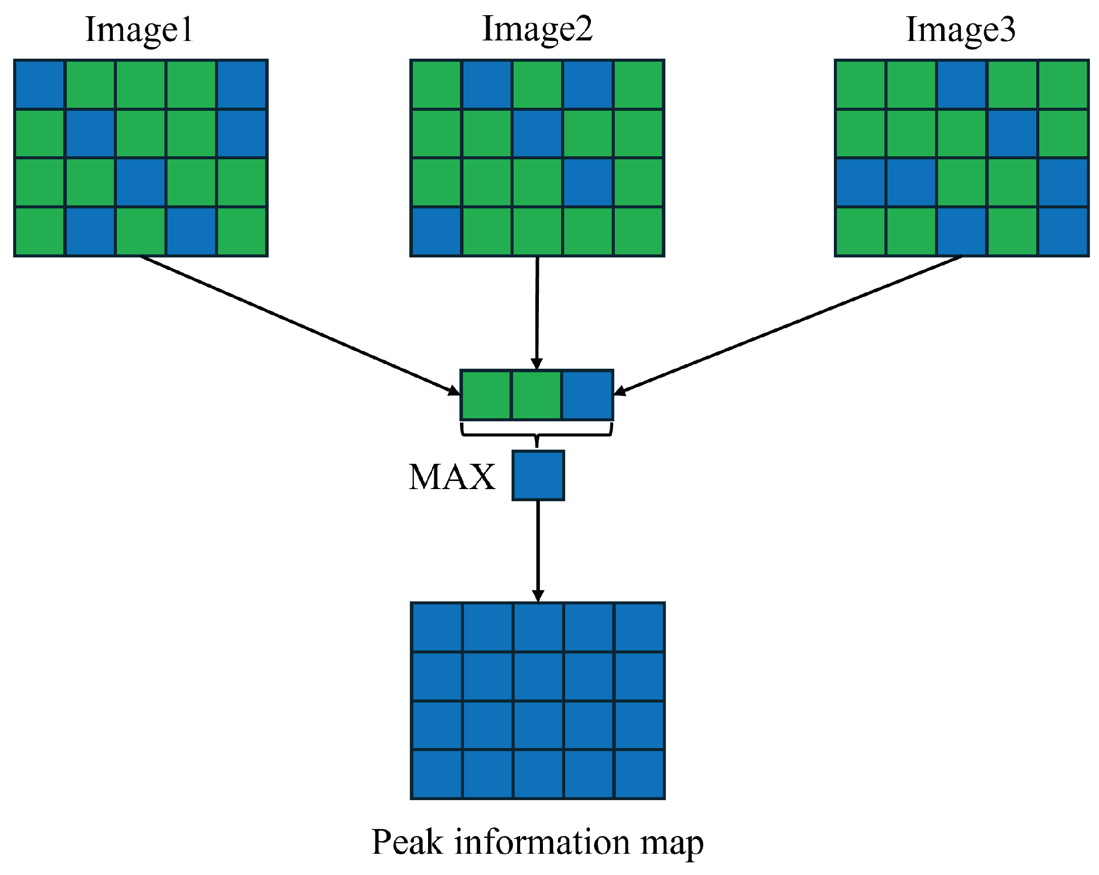
• We introduce the concept of peak information maps and design a corresponding method for calculating peak information maps.
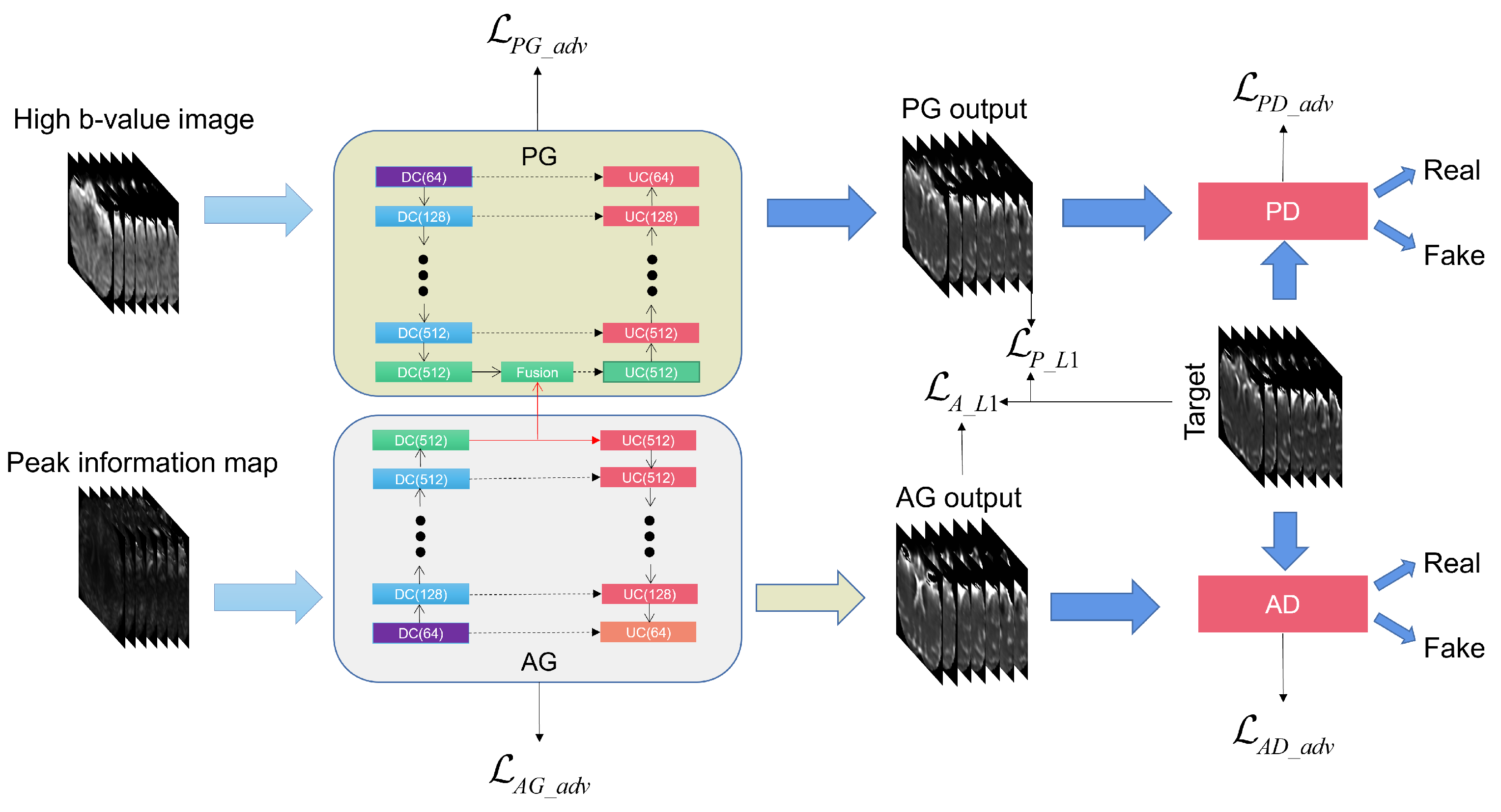
• We propose a novel end-to-end primary-auxiliary dual GAN network to translate high b-value images to low b-value images. In this network, the auxiliary generator extracts latent space features from peak information maps and transfers these features to the primary generator. The primary network integrates the latent space features and multi-scale features to generate low b-value images.
• Through DTI estimation and Xtract probabilistic tractography experiments, we validate the effectiveness of generating low b-value images for augmenting original dMRI data, providing new validation approaches for quality assessment in brain science research and offering optimized dMRI data for brain science studies.

2. Materials and Methods

2.1. Datasets

We obtained human brain dMRI images from the WU-Minn public dataset released by the Human Connectome Project (HCP) in 2016 [36]. We selected 96 dMRI data with the following specific parameters: echo-planar imaging (EPI) sequence, TR/TE = 5520/89.5 ms, flip angle (FA) = 78°, and voxel resolution of 1.25 × 1.25 × 1.25 mm.

We used the publicly accessible macaque brain imaging dataset from The PRIMatE Data Exchange (PRIME-DE) [6]. This dataset contains data from different sites, and we collected 8 data samples from Aix-Marseille Université (AMU), 12 data samples from Mount Sinai School of Medicine-Philips (MountSinai-P), 5 data samples from Mount Sinai School of Medicine-Siemens (MountSinai-S), 38 data samples from University of California, Davis (UCDavis), and 582 data samples from University of Wisconsin–Madison (UWM). The parameters of macaque datasets from different sites are shown in

Table 1. Specific parameters of macaque datasets.

Datasets	Scanner (3T)	Voxel Resolution (mm)	TE (ms)	TR (ms)	b-Values (s/mm2)
AMU	Siemens Prisma	1 × 1 × 1	87.6	7520	5, 500
MountSinai-P	Philips Achieva	1.5 × 1.5 × 1.5	19	2600	0, 1000
MountSinai-S	Siemens Skyra	1.0 × 1.0 × 1.0	95	5000	10, 1005
UCDavis	Siemens Skyra	1.4 × 1.4 × 1.4	115	6400	5, 1600
UWM	GE DISCOVERY_MR750	2.1875 × 3.1 × 2.1875	94.3	6100	0, 1000

. These datasets all suffer from varying degrees of imbalance between the number of low b-value and high b-value images. The quantities and ratios of low b-value images to high b-value images in the dMRI images from different data sites are shown in

Table 2. The number of low b-value and high b-value images in the macaque dataset.

Datasets	Number of Low b-Value Images	Number of High b-Value Images	Ratio
AMU	4	67	1:17
MountSinai-P	2	120	1:60
MountSinai-S	10	80	1:8
UCDavis	6	60	1:10
UWM	1	12	1:12

.

2.2. Preprocessing

The series of preprocessing steps applied to all the datasets are as follows:

• Head motion correction and eddy current correction were performed using the FSL tool.
• Non-brain tissues were removed from human brain images using the FSL tool, while non-brain tissues were removed from macaque brain images using a deep learning method developed by our research group [37].
• Paired high b-value and low b-value images were extracted from the dMRI images, where the high b-value images served as inputs to the model, and the low b-value images served as reference images. The task of extracting b-value images was accomplished using the FSL tool.
• All high b-value images were scaled to the range of 0 to 1 using the min–max normalization method, and their dimensions were resampled to 256 × 256 × 256.
• The data were divided into pre-training, training, and testing sets: the pre-training set included 96 pairs of human brain images and 467 pairs of UWM images. The remaining data from UWM, AMU, MountSinai-P, MountSinai-S, and UCDavis sites were divided into training and testing sets, with a ratio of 8:2.

2.3. PadGAN

We propose a primary-auxiliary dual generative adversarial network called PadGAN, consisting of two generative adversarial networks: the primary network and the auxiliary network, both targeting the domain of low b-value images. Figure 1 illustrates the training data flow of PadGAN. During training, the peak information map is input into the auxiliary generator, which learns towards the domain of low b-value images through adversarial learning while simultaneously passing latent space features to the primary generator. The high b-value images are input into the primary generator, which maps them to the domain of low b-value images through feature fusion modules by merging latent space features. The low b-value images generated by the auxiliary generator and the primary generator are passed to the auxiliary discriminator and the primary discriminator, respectively, to discriminate between real and generated images, thereby enhancing the generation capabilities of both generators through adversarial learning.

2.3.1. Peak Information Maps

Recently, latent space has flourished in the field of image generation [38]. Latent space can generate diverse high-resolution images [39] and can also be used for re-editing images by extracting latent space features [40,41]. In order to introduce diversity into generated images, random Gaussian noise is commonly used as the input for extracting latent space features. However, unlike works focused on enhancing image diversity, this paper places high demands on the accuracy of generated image details. Therefore, random Gaussian noise as the input for latent space feature extraction may not be suitable.

Max-pooling layers are widely used in image classification, segmentation, and other fields [42]. They can preserve texture features and edge information of images while reducing information redundancy. However, there is also a risk of losing important information. Due to the high demand for image details in end-to-end image-to-image translation tasks, max-pooling layers are rarely used to prevent information loss during training [43]. To reduce the risk of losing other information while preserving texture and other detailed information, we introduced the concept of peak information maps.

Given the assumption that brain images from the same data site and the same species exhibit a certain degree of similarity, we perform a per-pixel maximum extraction operation on the low b-value brain images of macaques within the same site. All extracted maximum values are concatenated into a 3D image, which represents the peak information map of that site, as illustrated in Figure 2. Additionally, Equations (1) and (2) demonstrate this process. The peak information maps from different sites serve as inputs to the auxiliary network for the respective site’s data, facilitating the extraction of latent space features.

$$vo{x}_{ij}=MAX(im{g}_{i1}\left(vo{x}_j\right),im{g}_{i2}\left(vo{x}_j\right),\dots im{g}_{in}\left(vo{x}_j\right))$$

(1)

$$re{f}_i=PConcat\left(vo{x}_{ij}\right),i=1,2,\dots ,k,j=1,2,\dots ,m.$$

(2)

where $vo{x}_{ij}$ represents the j-th voxel selected at the i-th site, $MAX(·)$ represents the peak extraction operation, $im{g}_{in}\left(vo{x}_j\right)$ represents the j-th pixel of the n-th image at the i-th site, and $re{f}_i$ represents the peak information map of the i-th site, of which there are k such peak information maps. $PConcat(·)$ represents the pixel concatenation operation, which concatenates individual pixels into the entire image. Iterate over all i and j values to obtain the peak information map for each site.

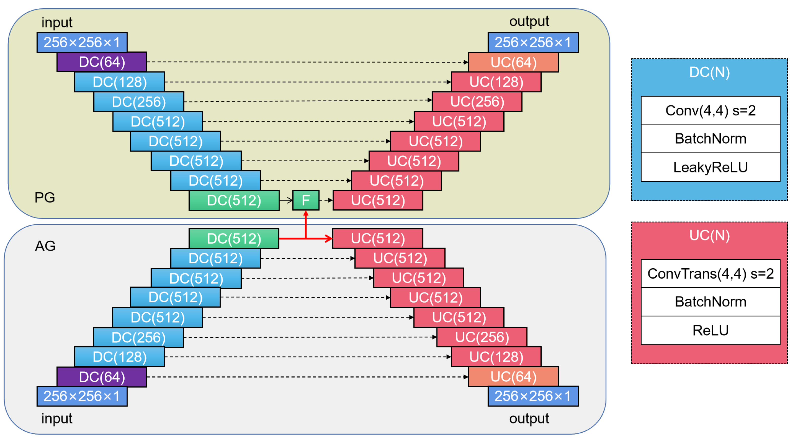
2.3.2. Auxiliary GAN

In the field of image generation, there is typically no end-to-end training data accessible. The extraction of latent space features is often achieved through several fully connected layers to decouple Gaussian noise and generate more diverse images [39]. The peak information map proposed in this paper provides end-to-end training data for extracting latent space features. We adopted an adversarial learning approach to extract latent space features to enhance the details of the generated images.

The role of the auxiliary generative adversarial network is to provide high-quality latent space information to the primary generative adversarial network. To achieve this, the auxiliary GAN continuously maps from the peak information map to the low b-value images through adversarial learning. The main architecture of the auxiliary generator network adopts a U-Net convolutional neural network, which is divided into an encoder and a decoder. The encoder consists of 8 down-sampling convolutional blocks, while the decoder consists of 8 up-sampling convolutional blocks. After encoding through the 8 down-sampling convolutional blocks, the input data obtain a 512 × 1 × 1 latent space feature, as shown in Equation (3).

$$Latent=8\ast DC\left(x\right)$$

(3)

where $Latent$ represents latent space features, $8\ast DC(·)$ represents the 8 down-sampling convolution operations, and x represents the input image, where the output of each down-sampling convolution operation serves as the input to the next down-sampling convolution operation. The specific down-sampling convolution operation is shown in Equation (4).

$$fea=LReLU\left(BN\right(Conv\left(input\right)\left)\right)$$

(4)

where $fea$ represents the feature map obtained from a down-sampling convolution operation $DC(·)$, $LReLU(·)$ represents the LeakyReLU activation function, $BN(·)$ represents the batch normalization operation, and $Conv(·)$ represents the convolution operation with a kernel size of 4 × 4, stride of 2, and padding of 1. $input$ denotes the input image or feature map. It should be noted that there is no activation function operation in the first down-sampling convolutional layer, and the ReLU activation function is used instead of LeakyReLU in the last down-sampling convolutional layer.

The latent space features have two destinations: The first one is sent to the primary network to enhance its generation capability, and the second one is sent to the auxiliary network to strengthen the inherent properties of the latent space features. Within the auxiliary network, 8 up-sampling convolution modules decode the latent space features and map them to the low b-value space, as shown in Equation (5).

$$\widehat{y}=8\ast UC\left(Latent\right)$$

(5)

where $\widehat{y}$ represents the output image of the auxiliary generator, and $8\ast UC(·)$ denotes 8 up-sampling transpose convolution operations, where the output of each up-sampling transpose convolution operation serves as the input to the next up-sampling transpose convolution operation. The specific details of the up-sampling transpose convolution operation are outlined in Equations (6) and (7).

$$fe{a}_{Ci}=\left\{\begin{array}{c}fe{a}_{DC(9-i)},i=1\hfill \\ Concat(fe{a}_{DC(9-i)},fe{a}_{UC(i-1)}),i=2,3,\dots ,8\hfill \end{array}\right.$$

(6)

$$fe{a}_{UCi}=\left\{\begin{array}{c}ReLU\left(BN\left(ConvT\left(fe{a}_{Ci}\right)\right)\right),i=1,2,\dots ,7\hfill \\ Tanh\left(ConvT\left(fe{a}_{Ci}\right)\right),i=8\hfill \end{array}\right.$$

(7)

where $fe{a}_{DC(9-i)}$ represents the features of the (9-i)-th down-sampling convolutional module, and $fe{a}_{UCi}$ represents the features of the i-th up-sampling transpose convolutional module. $Concat(·)$ represents the operation of concatenating feature dimensions. If this is the first up-sampling transpose convolutional module, the $Concat(·)$ operation is ignored. $ReLU(·)$ represents the ReLU activation function, and $ConvT(·)$ denotes the transpose convolution operation, with a kernel size of 4 × 4, a stride of 2, and padding of 1. $Tanh(·)$ represents the Tanh activation function. It is worth noting that different equations are executed for different values of i, and finally, when $i=8$, the final generated image is output.

The discriminator of the auxiliary generator adopts the PatchGAN architecture [13], which consists of 5 convolutional layers. Each convolutional layer performs down-sampling on the feature map. Eventually, it obtains a feature map size that is $\frac{1}{2^5}\times \frac{1}{2^5}$ times larger than the original image, where each intensity value in this feature map corresponds to the discriminative result of a certain region in the input image. PatchGAN divides the image into small patches for discrimination, which allows for accurate reflection of local information and enhances accuracy.

2.3.3. Primary GAN

The generator of the primary network consists of down-sampling convolutional blocks, feature fusion modules, and up-sampling convolutional blocks. The down-sampling convolutional blocks and up-sampling convolutional blocks have the same architecture as those in the auxiliary generator, with the only difference being that the input to the primary generator is the high b-value image. The details and connections between the auxiliary generator and the primary generator are illustrated in Figure 3. The feature fusion module combines the encoded features from the auxiliary network’s latent space and the primary generator, as specified in Equation (8).

$$fe{a}_{out}=Fusion(Latent,fe{a}_{MDC})$$

(8)

where $Fusion(·)$ represents the feature fusion operation, $Latent$ denotes the latent space feature map from the auxiliary generator, $fe{a}_{MDC}$ represents the encoded features from the primary generator, and $fe{a}_{out}$ represents the output feature map after the fusion operation. The specific feature fusion operation is illustrated in Equations (9) and (10).

$$fe{a}_{Cout}=Concat(Latent,fe{a}_{MDC})$$

(9)

$$fe{a}_{out}=ReLU\left(Linear\left(fe{a}_{Cout}\right)\right)$$

(10)

where $Linear(·)$ denotes the linear fusion operation. The linear layer not only reduces the dimensionality of the features but also effectively integrates the useful features according to weights. $fe{a}_{Cout}$ represents the output features after the concatenation operation.

The latent space features and the features from the primary generator are combined through the feature fusion module to obtain richer texture details. After passing through the feature fusion module, the features are processed by 8 up-sampling convolutional modules to output the generated images. During the training process, the generated images and the real images are evaluated by the primary discriminator, promoting the model’s generation capability through adversarial learning. Similar to the architecture of the auxiliary generator’s discriminator, the primary discriminator also adopts the PatchGAN network.

2.3.4. Loss

The loss function consists of both the primary network loss and the auxiliary network loss. Both are trained together but independently backpropagated. The loss function equations of the primary network and the auxiliary network are the same and include both generator adversarial loss, discriminator adversarial loss, and pixel reconstruction loss. Equation (11) represents the generator adversarial loss:

$${\mathcal{L}}_{G\_adv}=E{[D(x,G\left(x\right))-1]}^2$$

(11)

where ${\mathcal{L}}_{G\_adv}$ represents the generator adversarial loss, $E(·)$ denotes the expectation, $D(·)$ represents the discriminator’s output result, x denotes the input image, and $G\left(x\right)$ represents the generator’s output result. Theoretically, the generator’s adversarial loss is minimized when the discriminator identifies the generated result as 1. Equation (12) shows the discriminator adversarial loss:

$${\mathcal{L}}_{D\_adv}=E{[D(x,y)-1]}^2+E{\left[D(x,G\left(x\right))\right]}^2$$

(12)

where ${\mathcal{L}}_{D\_adv}$ represents the discriminator adversarial loss and y represents the real image. The discriminator adversarial loss consists of two parts: the first part minimizes when the concatenated real image with the source image dimension, after being passed through the discriminator, approaches 1; the second part minimizes when the concatenated generated image with the source image dimension, after being passed through the discriminator, approaches 0.

The generator loss and discriminator loss have opposite objective functions, and, during training, one should be fixed while the other is trained in an alternating manner to achieve the adversarial goal. Furthermore, to enhance the authenticity of the generated images, pixel-wise reconstruction loss should be introduced, as shown in Equation (13):

$${\mathcal{L}}_1={E[\parallel y-G\left(x\right)\parallel }_1]$$

(13)

where ${\mathcal{L}}_1$ represents the pixel-wise reconstruction loss and ${\parallel ·\parallel }_1$ represents the L1 norm. Therefore, the overall loss for both the main network and the auxiliary network is represented as Equation (14):

$$\mathcal{L}={\lambda }_{L1}{\mathcal{L}}_1+{\lambda }_{adv}({\mathcal{L}}_{G\_adv}+{\mathcal{L}}_{D\_adv})$$

(14)

where $\mathcal{L}$ represents the overall loss, ${\lambda }_{L1}$ represents the pixel-wise reconstruction loss coefficient, and ${\lambda }_{adv}$ represents the adversarial loss coefficient.

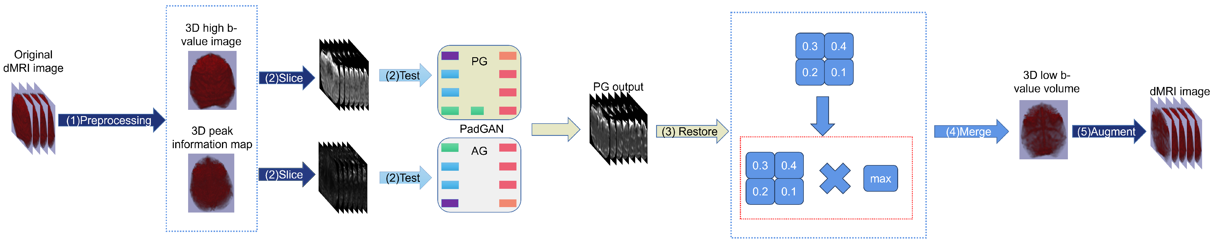
2.4. Process of dMRI Images Augmentation

After training, the entire dMRI image augmentation process using the final PadGAN model is as follows:

• Preprocess the dMRI images.
• Segment the data into 2-dimensional images along the second dimension and input them into PadGAN for processing to generate low b-value images.
• Multiply the generated images’ signal intensity values by the maximum value of the images before normalization to restore the original signal intensity range.
• Merge the generated two-dimensional images into three-dimensional images and resample all data to the original size.
• The synthesized three-dimensional images are incorporated into the 4-D dMRI images using FSL tools, effectively improving the quality of the dMRI data. The entire process is illustrated in Figure 4.

3. Results

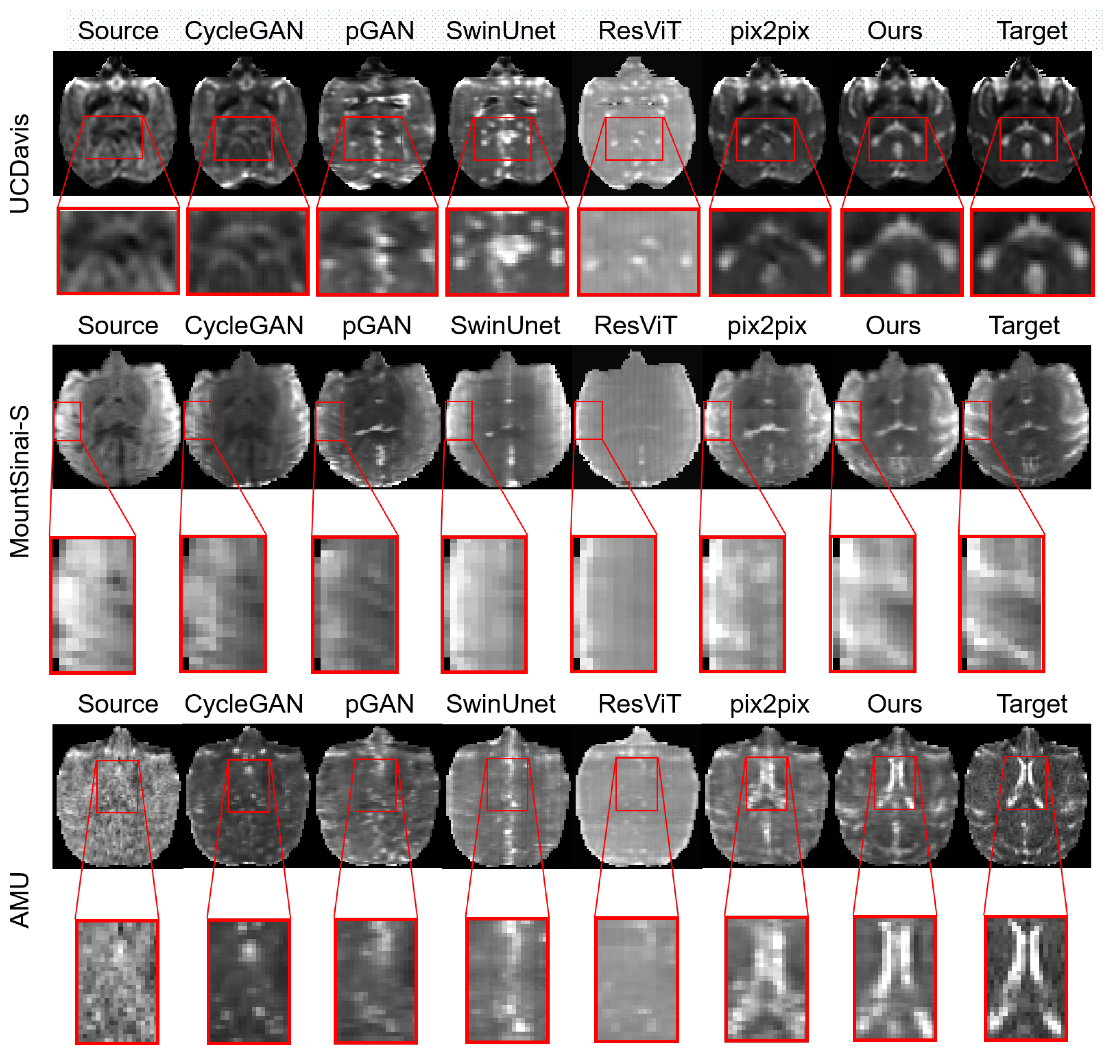
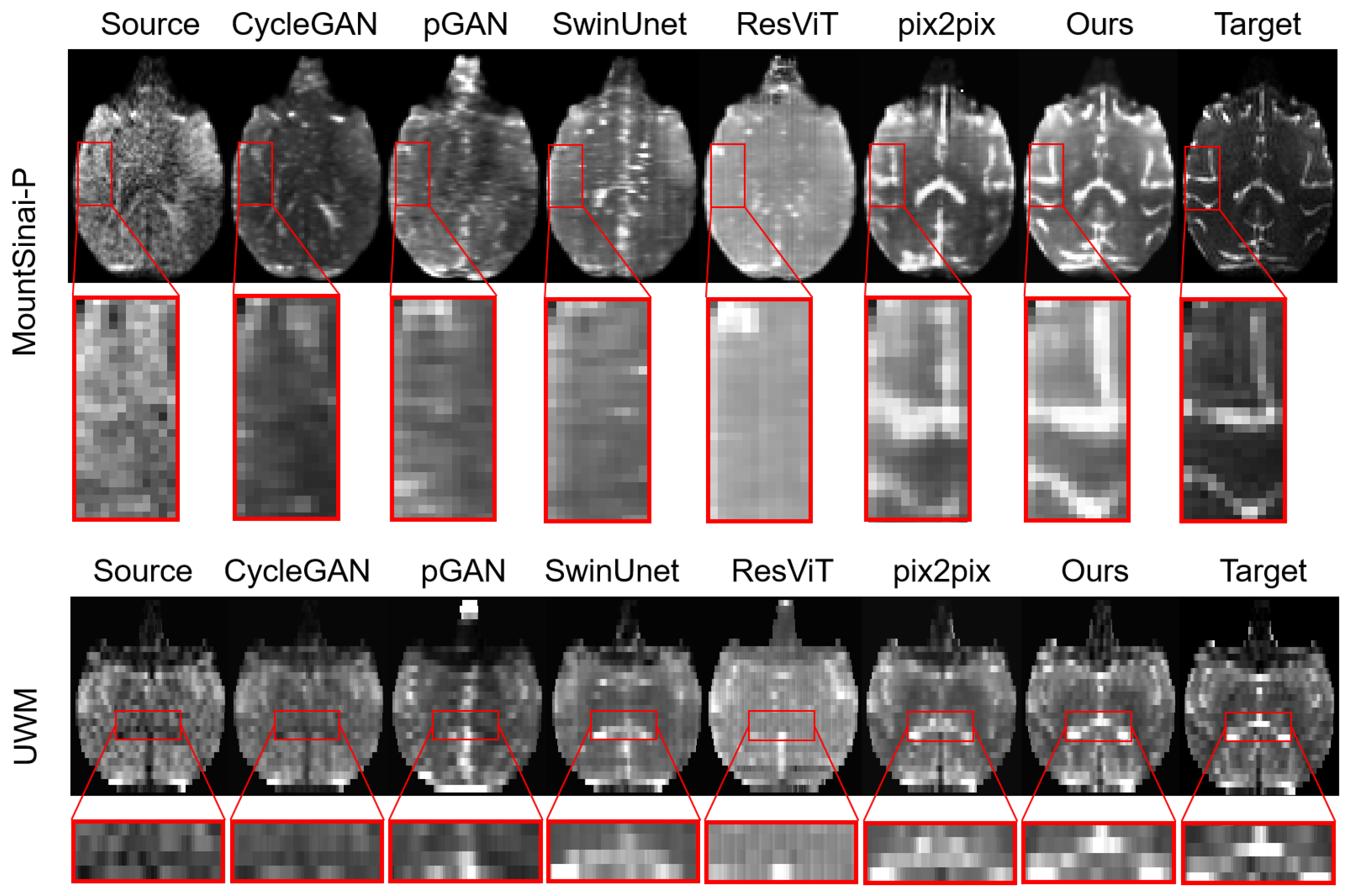
3.1. Comparison Experiments and Results

The method proposed in this paper is compared with five existing methods that have shown good performance in the field of medical image-to-image translation research. Specifically:

• Pix2pix [13] network adopts the U-Net architecture as the main framework of the generator.
• CycleGAN [14] network shares the same generator architecture as pix2pix, but it involves two generators and two discriminators for cyclic generation tasks.
• SwinUnet [24] utilizes the Swin Transformer as the main framework for medical image segmentation tasks, adapted for application in this paper.
• ResViT [26] builds upon the Vision Transformer architecture as the main generator framework.
• pGAN [30] adopts ResNet as the main framework.

For the comparative experiments, the original models’ architectures and training parameters are used during the training process. All models are pre-trained for 20 epochs and trained for an additional 80 epochs on an NVIDIA GeForce RTX 3090. Structural similarity (SSIM), peak signal-to-noise ratio (PSNR), and mutual information (MI) are selected as quantitative evaluation metrics in this paper.

Table 3. Quantitative comparison results including non-brain tissue.

Methods	PSNR	SSIM	MI
pix2pix	33.7100	0.9285	1.4313
CycleGAN	28.7177	0.8681	1.3716
pGAN	25.9224	0.8534	1.3467
SwinUnet	28.7114	0.8799	1.3786
ResViT	24.6464	0.8428	1.3614
Ours	38.8700	0.9556	1.5005

The bold font indicates the best result.

lists the comprehensive results of the AMU, Mount Sinai-P, Mount Sinai-S, UCDavis, and UWM sites, each containing non-brain tissue. To compare the results with only brain tissue, the non-brain tissue is removed from all results, as shown in

Table 4. Quantitative comparison of non-brain tissue removal.

Methods	PSNR	SSIM	MI
pix2pix	27.6511	0.7683	1.3144
CycleGAN	22.7904	0.5211	1.2528
pGAN	20.0104	0.4600	1.2275
SwinUnet	23.0855	0.5583	1.2623
ResViT	18.7379	0.4161	1.2376
Ours	32.2587	0.8822	1.3828

The bold font indicates the best result.

, which displays the results after excluding non-brain tissue for the five sites. The overall results are consistent with Table 1, but there is a slight decrease. Subsequent experiments show results after excluding non-brain tissue. The specific results for the five datasets are shown in

Table 5. Quantitative comparison between PadGAN and other translation frameworks across five independent sites.

Model	UCDavis			MountSinai-P			MountSinai-S			AMU			UWM
	PSNR	SSIM	MI	PSNR	SSIM	MI	PSNR	SSIM	MI	PSNR	SSIM	MI	PSNR	SSIM	MI
pix2pix	29.0037	0.7994	1.3353	22.4200	0.6227	1.2560	25.9427	0.8027	1.3347	29.6144	0.7919	1.2938	29.0558	0.8367	1.3045
CycleGAN	23.1076	0.5038	1.2514	19.4039	0.3975	1.2299	25.2008	0.6765	1.2872	26.2187	0.7005	1.2778	19.1597	0.4966	1.2367
pGAN	19.2235	0.4242	1.2284	19.9858	0.4199	1.2128	23.8789	0.6279	1.2511	22.0872	0.5719	1.2402	18.0913	0.4958	1.2018
SwinUnet	23.3034	0.5619	1.2584	17.4287	0.3400	1.2495	25.9383	0.7381	1.2993	26.8461	0.6911	1.2759	28.1703	0.7316	1.2662
ResViT	17.4558	0.3666	1.2398	20.1088	0.4487	1.2268	23.9303	0.5899	1.2568	20.2219	0.4879	1.2489	16.8820	0.4320	1.2023
Ours	35.7479	0.9188	1.4185	24.7701	0.8027	1.3379	30.6730	0.9068	1.3826	28.9085	0.8150	1.3033	29.5930	0.8753	1.3229

The bold font indicates the best result.

, and Figure 5 and Figure 6. The CycleGAN method produces results closer to the source images on most datasets. Although this method employs a dual-generator and dual-discriminator structure, with each generative adversarial network serving separate tasks for generating target and source images, it is suitable for scenarios where paired images are not required in both domains. In contrast, both generative adversarial networks in our method are dedicated to generating low b-value images, resulting in better visual observations and evaluation metrics. The pGAN method fails to generate detail-rich images, as it uses ResNet as the basic generator architecture with a deeper network structure, but lacks the capability to retain encoder feature map information like U-Net. Our method utilizes the advantages of the U-Net architecture to capture features from different layers, thereby preserving detailed image information. Transformer-based ResViT and SwinUnet methods exhibit relatively generic performance due to the differences in global information from different sites in the macaque brain image dataset and the limited data samples. In contrast, our method, a fully convolutional neural network, maximizes the local generation capabilities of convolutional neural networks. The Pix2pix method, a single generator adversarial network based on the U-Net generator architecture, performs well in generating global structural features but lacks detailed features. Our method addresses this limitation by using the auxiliary generative adversarial network to provide hidden space containing more detailed features, thus compensating for the shortcomings of the single generator adversarial network in capturing detailed features.

3.2. Ablation Experiments and Results

We conducted three ablation experiments to further investigate the role and effectiveness of the auxiliary generator in our proposed method. The details of the experiments are as follows: (1) removing the auxiliary network and retaining only the encoder part of the auxiliary network to encode the peak information map, to verify the role of the auxiliary network; (2) replacing the latent space features extracted by the auxiliary generator with random Gaussian noise to explore the role of latent space features; and (3) directly reusing the weights of the main generator in the auxiliary network to verify whether the auxiliary network needs to be trained separately.

The results are shown in

Table 6. Quantitative comparison of ablation experiments.

Methods	PSNR	SSIM	MI
PadGAN	32.3856	0.8825	1.3857
Setting (1)	27.2600	0.7600	1.3121
Setting (2)	28.1565	0.8176	1.3412
Setting (3)	30.5229	0.8440	1.3486

The bold font indicates the best result.

. (1) After removing the auxiliary network, PSNR decreased by 5.1256, SSIM decreased by 0.1225, and MI decreased by 0.0736. This indicates that the auxiliary generator plays an important role in improving the network performance. (2) When replacing the auxiliary generator with noise, PSNR decreased by 4.2291, SSIM decreased by 0.0649, and MI decreased by 0.0445. This suggests that the auxiliary generator can effectively extract latent space features from the peak information map. (3) When reusing the main network’s network weights in the auxiliary network, PSNR decreased by 1.8627, SSIM decreased by 0.0385, and MI decreased by 0.0371, fully demonstrating that the latent space learned by the auxiliary generator is different from that of the main generator, and the auxiliary generator has a necessary existence.

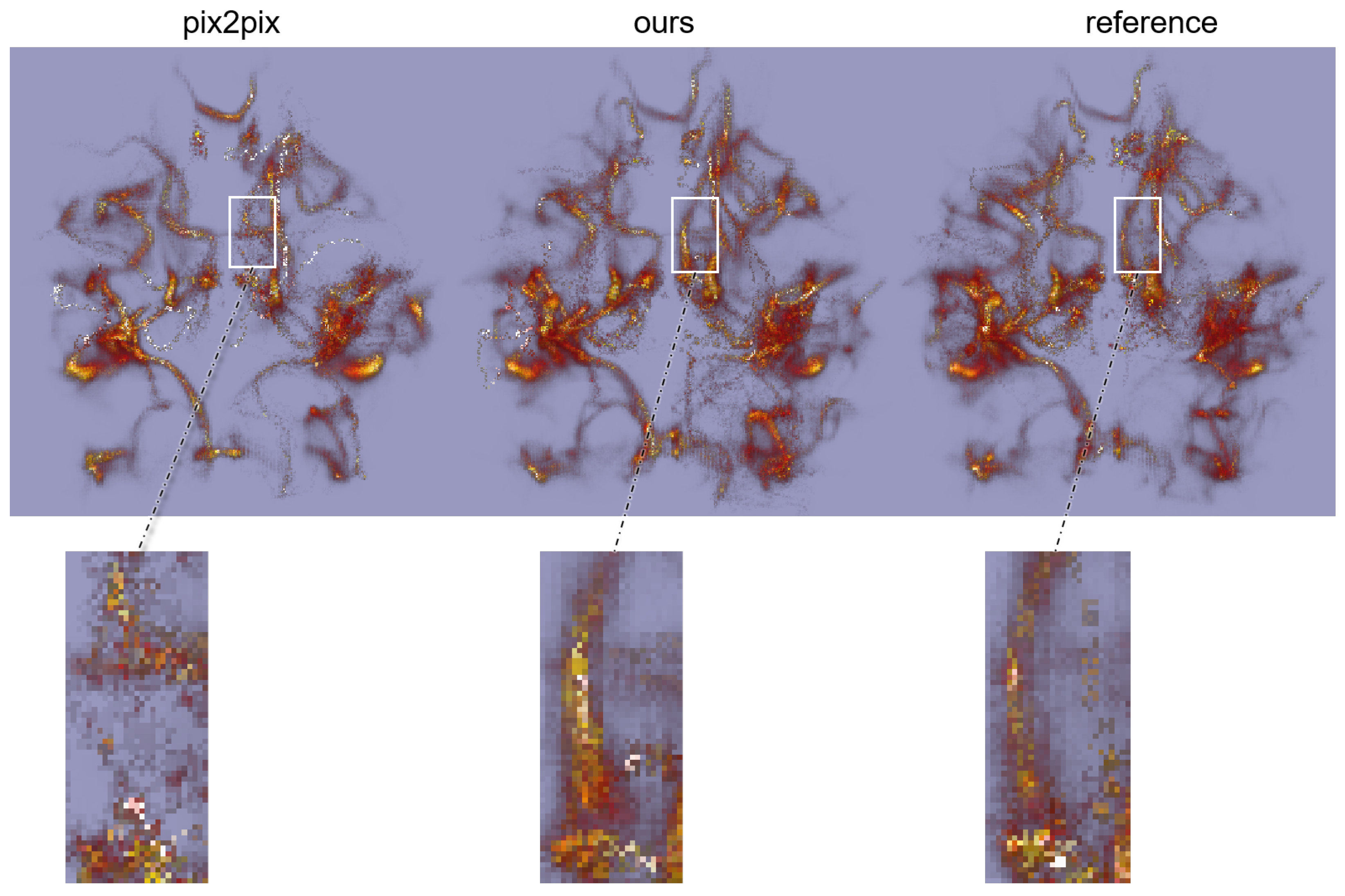
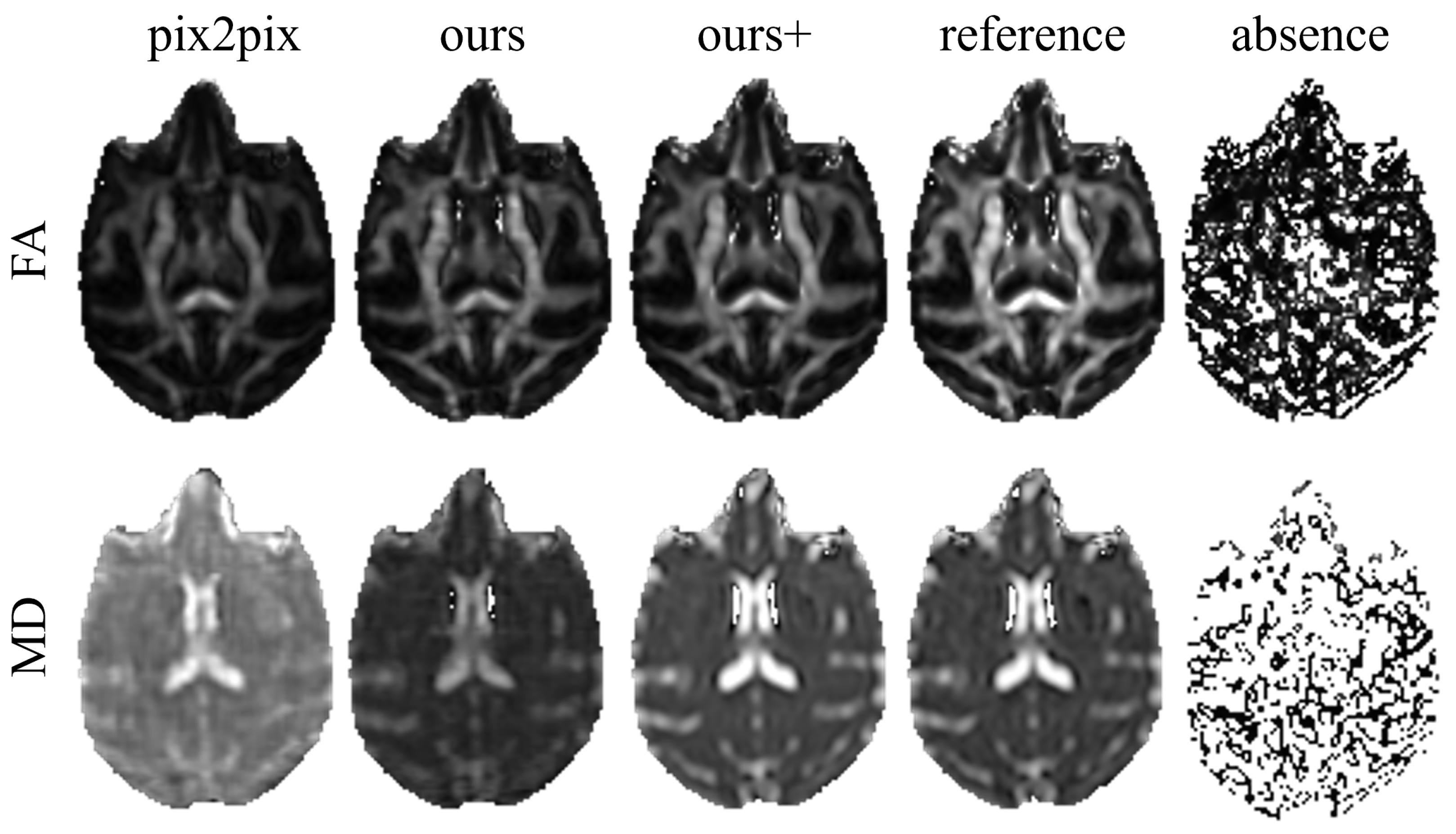
3.3. Xtract and DTI Estimation Results

Xtract is a robust probabilistic tractography method integrated into the FSL6.0 software package. It utilizes dMRI data to estimate the trajectories and connectivity patterns of white matter tracts. To assess the effectiveness of the augmented macaque dMRI brain images through our proposed method, we employed Xtract to compute the structural connectivity of dMRI brain images. Eight subjects were selected from the UCDavis dataset, and the images generated by pix2pix and PadGAN were respectively added to the corresponding dMRI data. Subsequently, we conducted Xtract tractography experiments on the dMRI images augmented by the pix2pix and PadGAN methods, as well as the original reference dMRI images, resulting in a total of 42 fiber tracts.

As shown in Figure 7, the fiber bundle visualization results demonstrate that, compared with pix2pix, our method captures more fiber bundles visually, and the shapes are similar to the reference results. It is worth noting that our results display more and clearer fiber bundles within the white rectangular area.

DTI is a magnetic resonance imaging technique used to study the diffusion properties of water molecules within tissues. DTI offers various diffusion parameters, with the most commonly used being fractional anisotropy (FA) and mean diffusivity (MD). FA represents the degree of directional diffusion of water molecules within the tissue, while MD represents the average strength of water molecule diffusion. To better evaluate the quality of the generated images, this study conducted DTI estimation on dMRI images augmented by the PadGAN and pix2pix methods. Figure 8 displays the DTI estimation results using FA and MD as examples. In the low b-value replacement experiment, our method demonstrates higher similarity to the original reference dMRI images compared with the pix2pix method. In the experiment of augmenting the original reference dMRI, our method shows smoother results. The last column in the figure demonstrates that the absence of low b-value volumes in dMRI images significantly affects the DTI estimation results. Therefore, low b-value images are crucial for DTI computation.

The experiments above indicate that Xtract and DTI estimation results can reflect the quality of different macaque image generation methods. Therefore, Xtract and DTI estimation are expected to become further validation methods for assessing the quality of generated macaque or medical images.

4. Discussion

In this work, we propose a method for dMRI brain image data augmentation using PadGAN to generate low b-value images. The introduction of peak information maps creates end-to-end conditions for extracting latent space features, allowing the auxiliary network to obtain latent space features through adversarial learning. On the basis of the U-Net network, a feature fusion module is added to the primary generator to merge latent space features and multi-scale information, thus generating images with rich details. Additionally, various generative adversarial network models are explored, and the strengths and weaknesses of each model are analyzed. PadGAN is creatively proposed and compared with comparative models in qualitative, quantitative, Xtract probabilistic tractography and DTI estimation to demonstrate its overall performance. Finally, ablation experiments are conducted on each module of PadGAN to demonstrate the importance of each part.

Both generators in PadGAN adopt the encoder–decoder architecture based on U-Net, preserving multi-scale information through skip connections, and the introduction of latent space features enables PadGAN to learn fine-grained image features. As shown in Figure 5 and Figure 6, unlike previous studies on human brain datasets where Transformer-based network models yield poor results, typically due to the large volume of data in human brain datasets resulting in different model parameters for each dataset, our approach uses a unified training strategy for the limited datasets of macaque brain images from each site. For datasets collected from each site, there are significant differences in acquisition parameters. Therefore, attention mechanisms are difficult to perform effectively for multi-site datasets. While ResNet can maintain model learning capability, even with deep network layers, it does not preserve multi-scale features like U-Net, resulting in deficiencies in detail generation. The pix2pix method based on U-Net demonstrates good performance, but, as a single generator and discriminator method, it still lacks in generating image details. Although CycleGAN has two generative adversarial networks, these networks are tasked with mutual conversion between two modal data samples and do not leverage both networks to generate images in one target domain. The auxiliary network in PadGAN provides latent space information to the primary network to enhance the detail generation of the generated images, utilizing U-Net’s skip connections to preserve multi-scale information, resulting in superior performance in image details.

Unlike the typical computer vision image-to-image translation domain, the signal intensity values of MRI images have absolute significance and can be used for DTI estimations or neuroimaging studies. Common images in daily life are usually RGB images with a maximum pixel intensity value of 255, while the signal intensity value range of macaque brain images is typically in the range of thousands to tens of thousands. Therefore, when evaluating the quality of MRI image generation, we can go beyond quantitative metrics and qualitative observations. For medical MRI, some researchers conduct Turing tests with expert radiologists to assess the authenticity of generated images [32]. For macaque and human brain images used in research, we can further evaluate the quality of generated images by calculating neural tracing or DTI estimation results, which presents a novel validation approach.

In future work, we can explore the generation of realistic images using multi-modal data. Although the macaque brain imaging dataset is limited, with few data within each site, many sites have at least two modalities of data. Utilizing network models that can effectively leverage multi-modal information may lead to the generation of higher quality images. Additionally, our method also has the potential for application in human brain imaging. Firstly, our method can be used for data augmentation of human brain dMRI images. Although human brain images typically have a higher spatial resolution and signal-to-noise ratio, and there are more publicly available datasets with better data quality, there may still be issues with insufficient collection of low b-value images due to operator and configuration issues. In such challenges, applying our method directly to human brain images is a good choice. Secondly, our method has the potential for application in classification studies of normal and diseased brain images. By using the PadGAN method to generate more images of a certain modality, the image sample size can be expanded, thereby improving classification accuracy. However, diseased images typically require higher precision in a certain region, and it may be a good choice to introduce attention mechanisms to enhance contextual information.

5. Conclusions

PadGAN is employed to translate high b-value images of macaque brains to low b-value images and augment dMRI image data. Visually, the low b-value images generated by PadGAN exhibit richer detail information. In terms of evaluation metrics, both image quality and structural similarity show significant improvement. Results from Xtract probabilistic tractography and DTI estimation indicate that the dMRI images obtained through our data augmentation method yield better outcomes. This work can provide data augmentation and optimization services for neuroscience, and also offers insights into quality assessment methods for macaque dMRI brain imaging data.

References

1. Passingham, R. How good is the macaque monkey model of the human brain? Curr. Opin. Neurobiol. 2009, 19, 6–11. [Google Scholar] [CrossRef]
2. Neubert, F.X.; Mars, R.B.; Sallet, J.; Rushworth, M.F. Connectivity reveals relationship of brain areas for reward-guided learning and decision making in human and monkey frontal cortex. Proc. Natl. Acad. Sci. USA 2015, 112, E2695–E2704. [Google Scholar] [CrossRef]
3. Wang, Q.; Wang, Y.; Chai, J.; Li, B.; Li, H. A review of homologous brain regions between humans and macaques. J. Taiyuan Univ. Technol. 2021, 52, 274–281. [Google Scholar]
4. Bauer, M.H.; Kuhnt, D.; Barbieri, S.; Klein, J.; Becker, A.; Freisleben, B.; Hahn, H.K.; Nimsky, C. Reconstruction of white matter tracts via repeated deterministic streamline tracking–initial experience. PLoS ONE 2013, 8, e63082. [Google Scholar] [CrossRef]
5. Soares, J.M.; Marques, P.; Alves, V.; Sousa, N. A hitchhiker’s guide to diffusion tensor imaging. Front. Neurosci. 2013, 7, 31. [Google Scholar] [CrossRef]
6. Milham, M.P.; Ai, L.; Koo, B.; Xu, T.; Amiez, C.; Balezeau, F.; Baxter, M.G.; Blezer, E.L.A.; Brochier, T.; Chen, A.H. An Open Resource for Non-human Primate Imaging. Neuron 2018, 100, 61–74.e2. [Google Scholar] [CrossRef]
7. Yurt, M.; Dar, S.U.; Erdem, A.; Erdem, E.; Oguz, K.K.; Cukur, T. mustgan: Multi-stream generative adversarial networks for mr image synthesis. Med. Image Anal. 2021, 70, 101944. [Google Scholar] [CrossRef]
8. Shin, H.C.; Ihsani, A.; Mandava, S.; Sreenivas, S.T.; Forster, C.; Cha, J. Ganbert: Generative adversarial networks with bidirectional encoder representations from transformers for mri to pet synthesis. arXiv 2020, arXiv:2008.04393. [Google Scholar]
9. Huang, J.H. Swin transformer for fast mri.Neurocomputing. Neurocomputing 2022, 493, 281–304. [Google Scholar] [CrossRef]
10. Sikka, A.; Virk, J.S.; Bathula, D.R. Mri to pet cross-modality translation using globally and locally aware gan (gla-gan) for multi-modal diagnosis of alzheimer’s disease. arXiv 2021, arXiv:2108.02160. [Google Scholar]
11. Goodfellow, I.J.; Pouget-Abadie, J.; Mirza, M.; Xu, B.; Warde-Farley, D.; Ozair, S.; Courville, A.; Bengio, Y. Generative Adversarial Networks. arXiv 2014, arXiv:1406.2661. [Google Scholar] [CrossRef]
12. Jiang, Y.F.; Chang, S.Y.; Wang, Z.Y. TransGAN: Two Pure Transformers Can Make One Strong GAN, and That Can Scale Up. arXiv 2021, arXiv:2102.07074. [Google Scholar]
13. Isola, P.; Zhu, J.Y.; Zhou, T.; Efros, A.A. Image-to-image translation with conditional adversarial networks. In Proceedings of the IEEE Conference on Computer Vision and Pattern Recognition, Honolulu, HI, USA, 21–26 July 2017; pp. 1125–1134. [Google Scholar]
14. Zhu, J.Y.; Park, T.; Isola, P.; Efros, A.A. Unpaired image-to-image translation using cycle-consistent adversarial networks. In Proceedings of the IEEE International Conference on Computer Vision, Venice, Italy, 22–29 October 2017; pp. 2242–2251. [Google Scholar]
15. Welander, P.; Karlsson, S.; Eklund, A. Generative adversarial networks for image-to-image translation on multi-contrast mr images-a comparison of cyclegan and unit. arXiv 2018, arXiv:1806.07777. [Google Scholar]
16. Gu, X.; Knutsson, H.; Nilsson, M.; Eklund, A. Generating diffusion mri scalar maps from t1 weighted images using generative adversarial networks. In Image Analysis; Lecture Notes in Computer Science (Including Subseries Lecture Notes in Artificial Intelligence and Lecture Notes in Bioinformatics); Springer: Cham, Switzerland, 2019; pp. 489–498. [Google Scholar]
17. Abramian, D.; Eklund, A. Generating fmri volumes from t1-weighted volumes using 3d cyclegan. arXiv 2019, arXiv:1907.08533. [Google Scholar]
18. Zhao, P.; Pan, H.; Xia, S. Mri-trans-gan: 3d mri cross-modality translation. In Proceedings of the 2021 40th Chinese Control Conference (CCC), Shanghai, China, 26–28 July 2021; pp. 7229–7234. [Google Scholar]
19. Armanious, K.; Jiang, C.M.; Abdulatif, S.; Kustner, T.; Gatidis, S.; Yang, B. Unsupervised Medical Image Translation Using Cycle-MedGAN. In Proceedings of the 2019 27th European Signal Processing Conference (EUSIPCO), A Coruña, Spain, 2–6 September 2019; pp. 1–5. [Google Scholar]
20. Benoit, A.R. Manifold-Aware CycleGAN for High-Resolution Structural-to-DTI Synthesis. In Computational Diffusion MRI: International MICCAI Workshop; Springer: Cham, Switzerland, 2021; pp. 213–224. [Google Scholar]
21. Kearney, V.; Ziemer, B.P.; Perry, A.; Wang, T.; Chan, J.W.; Ma, L.; Morin, O.; Yom, S.S.; Solberg, T.D. Attention-Aware Discrimination for MR-to-CT Image Translation Using Cycle-Consistent Generative Adversarial Networks. Radiol. Artif. Intell. 2020, 2, e190027. [Google Scholar] [CrossRef]
22. Bui, T.D.; Nguyen, M.; Le, N.; Luu, K. Flow-Based Deformation Guidance for Unpaired Multi-contrast MRI Image-to-Image Translation. In Proceedings of the Medical Image Computing and Computer Assisted Intervention—MICCAI 2020, Lima, Peru, 4–8 October 2020; pp. 728–737.
23. Zhang, H.; Li, H.; Parikh, N.A.; He, L. Multi-contrast mri image synthesis using switchable cycle-consistent generative adversarial networks. Diagnostics 2022, 12, 816. [Google Scholar] [CrossRef]
24. Cao, H.; Wang, Y.Y.; Chen, J.; Jiang, D.S.; Zhang, X.P.; Tian, Q.; Wang, M.N. Swin-unet: Unet-like pure transformer for medical image segmentation. In Proceedings of the European Conference on Computer Vision, Tel Aviv, Israel, 23–27 October 2022; pp. 205–218. [Google Scholar]
25. Huang, J.; Xing, X.; Gao, Z.; Yang, G. Swin Deformable Attention U-Net Transformer (SDAUT) for Explainable Fast MRI for explainable fast mri. In Proceedings of the International Conference on Medical Image Computing and Computer-Assisted Intervention, Singapore, 18–22 September 2022; pp. 538–548. [Google Scholar]
26. Dalmaz, O.; Yurt, M.; Cukur, T. ResViT: Residual vision transformers for multi-modal medical image synthesis. IEEE Trans. Med. Imaging 2022, 41, 2598–2614. [Google Scholar] [CrossRef]
27. Yan, S.; Wang, C.; Chen, W.; Lyu, J. Swin transformer-based GAN for multi-modal medical image translation. Front. Oncol. 2022, 12, 942511. [Google Scholar] [CrossRef]
28. Dosovitskiy, A.; Beyer, L.; Kolesnikov, A.; Weissenborn, D.; Zhai, X.; Unterthiner, T.; Dehghani, M.; Minderer, M.; Heigold, G.; Gelly, S.; et al. An Image is Worth 16x16 Words: Transformers for Image Recognition at Scale. arXiv 2021, arXiv:2010.11929. [Google Scholar]
29. Schilling, K.G.; Blaber, J.; Hansen, C.; Cai, L.; Rogers, B.; Anderson, A.W.; Smith, S.; Kanakaraj, P.; Rex, T.; Resnick, S.M.; et al. Distortion correction of diffusion weighted MRI without reverse phase-encoding scans or field-maps Distortion correction of diffusion weighted mri without reverse phase-encoding scans or field-maps. PLoS ONE 2020, 15, e0236418. [Google Scholar] [CrossRef]
30. Pgan Dar, S.U.; Yurt, M.; Karacan, L.; Erdem, A.; Erdem, E.; Cukur, T. Image synthesis in multi-contrast mri with conditional generative adversarial networks. IEEE Trans. Med. Imaging 2019, 38, 2375–2388. [Google Scholar]
31. Yu, B.T.; Zhou, L.P.; Wang, L.; Shi, Y.H.; Fripp, J.; Bourgeat, P. Ea-GANs: Edge-Aware Generative Adversarial Networks for Cross-Modality MR Image Synthesis. IEEE Trans. Med. Imaging 2019, 38, 1750–1762. [Google Scholar] [CrossRef] [PubMed]
32. Armanious, K.; Jiang, C.M.; Fischer, M.; Kustner, T.; Hepp, T.; Nikolaou, K.; Gatidis, S.; Yang, B. MedGAN: Medical image translation using GANs. Comput. Med. Imaging Graph. 2020, 79, 101684. [Google Scholar] [CrossRef] [PubMed]
33. Yang, Q.; Li, N.; Zhao, Z.; Fan, X.; Chang, E.; Xu, Y. Mri cross-modality image-to-image translation. Sci. Rep. 2020, 10, 3753. [Google Scholar] [CrossRef]
34. Warrington, S.; Bryant, K.L.; Khrapitchev, A.A.; Sallet, J.; Charquero-Ballester, M.; Douaud, G.; Jbabdi, S.; Mars, R.B.; Sotiropoulos, S.N. Xtract-standardised protocols for automated tractography in the human and macaque brain. NeuroImage 2020, 217, 116923. [Google Scholar] [CrossRef] [PubMed]
35. Jenkinson, M.; Beckmann, C.F.; Behrens, T.E.; Woolrich, M.W.; Smith, S.M. FSL. NeuroImage 2012, 62, 782–790. [Google Scholar] [CrossRef]
36. Van Essen, D.C.; Smith, S.M.; Barch, D.M.; Behrens, T.E.; Yacoub, E.; Ugurbil, K. The wu-minn human connectome project: An overview. NeuroImage 2013, 80, 62–79. [Google Scholar] [CrossRef] [PubMed]
37. Wang, Q.; Fei, H.; Abdu, N.S.; Xia, X.; Li, H. A Macaque Brain Extraction Model Based on U-Net Combined with Residual Structure. Brain Sci. 2022, 12, 260. [Google Scholar] [CrossRef] [PubMed]
38. Abdal, R.; Qin, Y.; Wonka, P. Image2stylegan: How to embed images into the stylegan latent space? In Proceedings of the IEEE/CVF International Conference on Computer Vision, Seoul, Republic of Korea, 27 October–2 November 2019; pp. 4432–4441. [Google Scholar]
39. Karras, T.; Laine, S.; Aila, T. A style-based generator architecture for generative adversarial networks. IEEE Trans. Pattern Anal. Mach. Intell. 2019, 43, 4217–4228. [Google Scholar] [CrossRef]
40. Wang, T.; Zhang, Y.; Fan, Y.; Wang, J.; Chen, Q. High-Fidelity GAN Inversion for Image Attribute Editing. In Proceedings of the IEEE/CVF Conference on Computer Vision and Pattern Recognition, New Orleans, LA, USA, 18–24 June 2022; pp. 11379–11388. [Google Scholar]
41. Richardson, E.; Alaluf, Y.; Patashnik, O.; Nitzan, Y.; Azar, Y.; Shapiro, S.; Cohen-Or, D. Encoding in Style: A StyleGAN Encoder for Image-to-Image Translation. In Proceedings of the IEEE/CVF Conference on Computer Vision and Pattern Recognition, Nashville, TN, USA, 20–25 June 2021; pp. 2287–2296. [Google Scholar]
42. Gholamalinezhad, H.; Khosravi, H. Pooling Methods in Deep Neural Networks, a Review. arXiv 2020, arXiv:2009.07485. [Google Scholar]
43. Radford, A.; Metz, L.; Chintala, S. Unsupervised Representation Learning with Deep Convolutional Generative Adversarial Networks. arXiv 2015, arXiv:1511.06434. [Google Scholar]
Figure 1. The training data flow diagram of PadGAN. The auxiliary discriminator (AD) discriminates between the images generated by the auxiliary generator (AG) and the real images, while the primary discriminator (PD) discriminates between the images generated by the primary generator (PG) and the real images. The auxiliary network uses three losses, L A G _ a d v , L A D _ a d v , and L A _ L 1 , for backpropagation, while the primary network uses three losses, L P G _ a d v , L P D _ a d v , and L A _ L 1 , for backpropagation.
Applsci 14 03229 g001
Figure 2. Schematic diagram of peak information map. Image1, Image2, and Image3 represent three images within the same site. The green and blue rectangles represent the pixels of the image, where the blue rectangles represent the maximum pixel values at the same position in the three images. Concatenating the maximum value pixels at each position yields the peak information map.
Applsci 14 03229 g002
Figure 3. The structure of the two generators. The upper part represents the primary generator (PG), while the lower part represents the auxiliary generator (AG). In the primary generator, the letter “F” represents the feature fusion layer, UC(N) represents the up-sampling transpose convolution operation, and DC(N) represents the down-sampling convolution operation. N represents the number of convolutional channels.
Applsci 14 03229 g003
Figure 4. The overall processing flow of dMRI images augmentation. The figure provides a detailed description of the steps outlined in Section 2.4. During testing, the auxiliary generator no longer outputs results, as there is no need to further optimize the latent space through backpropagation.
Applsci 14 03229 g004
Figure 5. Visualization of 3 site datasets. These are 3 randomly selected data samples from the 3 datasets. The first column represents the source image, the last column represents the target image, and the middle column represents the comparative result. The red box highlights some details.
Applsci 14 03229 g005
Figure 6. Visualization of 2 site datasets. These are 2 randomly selected data samples from the 2 datasets. The first column represents the source image, the last column represents the target image, and the middle column represents the comparative result. The red box highlights some details.
Applsci 14 03229 g006
Figure 7. Fiber bundle visualization results. The left and middle columns respectively show the results after data enhancement with the pix2pix and PadGAN methods, while the right column shows the results of the reference original dMRI image. The part inside the white rectangle is zoomed in for comparison.
Applsci 14 03229 g007
Figure 8. DTI estimation results. The first row displays FA, and the second row shows MD. The first and second columns respectively show the DTI estimation results after replacing the original low b-value volume with volumes generated using pix2pix and our method. The third column shows the DTI estimation results after augmenting the original reference dMRI images using our method for data augmentation. The fourth and fifth columns respectively display the DTI estimation results for the reference images and dMRI without the low b-value volume.
Applsci 14 03229 g008