Abstract
Considering the vulnerability of satellite positioning signals to obstruction and interference in orchard environments, this paper investigates a navigation and positioning method based on real-time kinematic global navigation satellite system (RTK-GNSS), inertial navigation system (INS), and light detection and ranging (LiDAR). This method aims to enhance the research and application of autonomous operational equipment in orchards. Firstly, we design and integrate robot vehicles; secondly, we unify the positioning information of GNSS/INS and laser odometer through coordinate system transformation; next, we propose a dynamic switching strategy, whereby the system switches to LiDAR positioning when the GNSS signal is unavailable; and finally, we combine the kinematic model of the robot vehicles with PID and propose a path-tracking control system. The results of the orchard navigation experiment indicate that the maximum lateral deviation of the robotic vehicle during the path-tracking process was 0.35 m, with an average lateral error of 0.1 m. The positioning experiment under satellite signal obstruction shows that compared to the GNSS/INS integrated with adaptive Kalman filtering, the navigation system proposed in this article reduced the average positioning error by 1.6 m.
1. Introduction
At present, China is the world’s largest producer and consumer of forest fruit [1], with the State Bureau of Statistics reporting that in 2021, orchards occupied approximately 12,962 thousand hectares, marking a 2.5% increase, and the annual fruit production in China was 296.11 million tons. However, compared with farmland production, the mechanization rate in orchards is low, and complex tasks such as picking, transportation, weeding, and pruning are common. The issue of seasonal employment makes it difficult to hire expensive workers, and the rising labor cost has become an important factor restricting the improvement of the forest and fruit industry. Therefore, it is vital to enhance the mechanization level of orchard industry and improve the efficiency of orchard operations [2,3,4]. In view of the unique advantages of intelligent operating equipment in complex agricultural production, autonomous navigation technology in orchards has become more and more widely used in recent years, and the orchard autonomous navigation technology has become an indispensable core technology in the intelligent operation equipment. The autonomous navigation technology of operational equipment involves its own precise positioning, path planning, path-tracking control, and other functions, which is an important prerequisite for realizing intelligent and efficient operation of orchard machinery.
The real-time kinematic global satellite navigation system (RTK-GNSS) is currently one of the most widely utilized navigation technologies. It achieves centimeter-level accuracy in satellite positioning by processing carrier phase measurements as a ranging source in open outdoor environments [5]. It provides real-time, absolute positioning with broad coverage, all-weather capabilities, and high precision [6,7,8]. However, the tree canopy and bird-proof nets block the satellite signals [5], making it difficult to ensure continuous high-precision autonomous movement. Therefore, it is necessary to integrate information from other sensors to overcome this drawback.
Recently, some robot navigation frameworks have been proposed based on combinations of different types of sensor information, including GNSS-INS [9,10], GNSS-Visual [11,12,13], and GNSS-LiDAR [14,15,16]. Among them, inertial navigation is widely used in the case of transient loss of satellite signals due to its advantages of isolation from the environment and high operational accuracy in a short period of time. Huang et al. [17] designed an integrated navigation system based on real-time dynamic kinematics BeiDou satellite navigation system (RTK-BDS) and INS and conducted navigation experiments using an agricultural machine to keep the position error within 3 cm on an open road. Sun et al. [18] fused the GNSS with Kalman-filter-processed inertial measurement unit (IMU) information for position estimation between GNSS position updates to improve the positioning accuracy. Chuang et al. [19] greatly improve the accuracy and robustness of high-precision localization in forests by utilizing GNSS/INS to obtain high-precision attitude and velocity information via fusion of the two sensors. Due to the accuracy limitation of inertial devices, INS has a drift error accumulated over time [20]. This drift makes INS unsuitable for orchard environments where satellite signals are blocked for extended periods, and the terrain is uneven and overgrown with weeds.
The positioning of a visual sensor is obtained by transforming the pixel position, pixel–camera distance, camera coordinate system, and robot coordinate system. Ball et al. [21] used a GNSS/INS-based navigation system and machine-vision-based obstacle monitoring to achieve normal operation and the obstacle avoidance function of the robot without a GNSS signal for five minutes. Zuo et al. [22] proposed a GNSS navigation method enhanced by vision, which uses a Kalman filter to integrate binocular vision with GNSS-provided positioning. This approach effectively reduces navigation errors when GNSS signals are disrupted by significant noise. Chu et al. [23] developed an integrated system comprising a camera, IMU, and GNSS, utilizing the extended Kalman filter (EKF). This integrated approach delivers precise position estimation and potentially surpasses the performance of tightly coupled GNSS/IMU systems, especially in challenging environments with limited GNSS observations. In the natural outdoor environment, visual sensors are susceptible to the influence of light. In addition, due to the large amount of image information captured by the visual sensors, a large amount of computing power is consumed [15].
The information gathered by light detection and ranging (LiDAR) is extensive. Its accuracy and robustness are contingent upon the feature information extracted through position analysis algorithms and intelligent point cloud matching algorithms. Shamsudin et al. [24] derived a weight function through the fusion of GPS and LIDAR-SLAM to ensure their respective advantages and realize the consistent construction of the map of the fire robot. Jiang et al. [25] propose a LiDAR-assisted GNSS/INS integrated navigation system to ensure continuous positioning in GNSS-available and GNSS-blocked scenarios for seamless train positioning. Elamin et al. [26] integrated GNSS and LiDAR into an unmanned aerial vehicle (UAV) mapping system to overcome the problem of massive and prolonged GNSS signal interruptions caused by GNSS antenna failures during data collection. For laser navigation techniques, LiDAR positioning adopts an idea similar to inertial navigation odometer, which also accumulates errors.
Although laser odometers have smaller accumulated errors than INS in orchard environments, long-term operation can still cause positioning information to shift. This issue is particularly pronounced during row changes. Therefore, this paper uses accurate GNSS positioning information in differential mode to correct the accumulated errors of the laser odometer.
In summary, this paper investigates a GNSS/INS/LiDAR navigation method for complex orchard environments characterized by dense canopies, changing light conditions, uneven terrain, and weeds. In the following sections, Section 2 describes the hardware and software design and construction of the orchard robot vehicle, the autonomous positioning methods based on multi-sensor fusion, and the design of the navigation control system. In Section 3, the experimental study verifies the effectiveness of the proposed navigation system. Finally, in Section 4 and Section 5, discussion and conclusions are presented to summarize the whole paper.
2. Materials and Methods
2.1. Orchard Robotic Vehicle Design
2.1.1. Hardware Integration of the Orchard Robotic Vehicle
Utilized in complex orchards, our robot features a tracked chassis, an industrial computer, GNSS antennas (T1 Receiver), a receiver (FRII-D-Plus-INS), servo motors, a motor driver (KYDBL4875-2E), LiDAR (RS-LiDAR-16), and a wireless radio (HX-DU1601D). The chassis has a 0.32 m track gauge and a 1.2 m track length. The T1 receiver, enabling RTCM3.3 and centimeter-level RTK positioning, provides full RTCM differential data. Equipped with a high-performance MEMS inertial device, the FRII-D-Plus-INS receiver supports differential positioning with under 1.5 cm accuracy. The HX-DU1601D boasts a robust design and supports features such as full-duplex communication, channel viewing, and power adjustment. It enables users to set frequencies between 410 and 470 MHZ, fitting for varied outdoor scenarios. The RS-LiDAR-16, employing hybrid solid-state LiDAR technology, includes 16 laser transceivers. It offers a maximum range of 150 m, precision within ±2 cm, a capacity of 300,000 points per second, 360° horizontal angles, and −15° to 15° vertical angles. The RS-LiDAR-16 projects high-frequency lasers through 16 rotating emitters to scan the environment continually, yielding 3D point cloud data and reflectivity via its ranging algorithms. The overall hardware assembly composition of the robotic vehicle is shown in Figure 1.
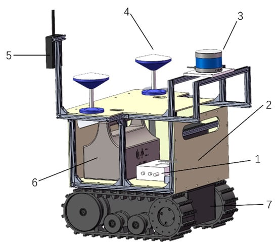
Figure 1.
Robotic vehicle overall hardware diagram. Note: 1. LiDAR; 2. GNSS antenna; 3. signal receiver; 4. industrial control unit; 5. GNSS/INS receiver; 6. mobile chassis; 7. mobile power supply.
2.1.2. Navigation System Design of the Orchard Robotic Vehicle
The framework of the automatic orchard navigation system is shown in Figure 2, which mainly focuses on the positioning unit, decision unit, and control unit. The localization unit consists of RTK-GNSS, LiDAR, and the inertial measurement unit, and provides the central control unit of the robot with localization information and RTK-GNSS signal status information. RTK-GNSS includes a wireless transmission radio, GNSS receiver, GNSS antenna, and GNSS base station. The decision unit is connected to each module through the serial port to process the positioning information. Firstly, based on RTK-GNSS status information, the system selects the appropriate navigation positioning mode. Next, it calculates the navigation path and determines the speeds of the left and right wheels using the PID control algorithm. Finally, the system issues control commands to the motion control module.
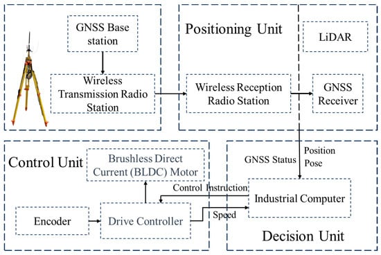
Figure 2.
GNSS-LiDAR fusion navigation framework.
The system software of the orchard mobile platform runs on the Linux operating system, using ROS as the software integration platform for the autonomous positioning and navigation system. The robot vehicle acquires and publishes the satellite-based self-positioning information and positioning status, as well as the LiDAR-based self-positioning information and positioning status, through the ROS-driven sensors. The information processing module subscribes to the sensor information through ROS and analyzes and processes the data. When the GNSS status, which indicates satellite positioning status information, is at 2, meaning the GNSS differential signal is good, the system navigates using GNSS positioning information. If the status is not 2, it switches to using laser odometer positioning information for navigation and positioning. After the information is processed and calculated, the system sends the robot’s motion control signals to the motion control module. Upon receiving the command, the drive controller activates the left and right brushless DC motors, causing the main control wheel to rotate and thereby controlling the movement of the robot vehicle. The overall architecture of the software system is depicted in Figure 3.
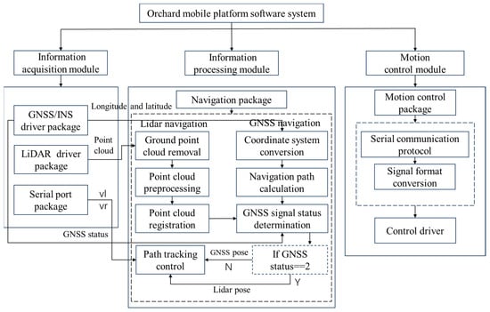
Figure 3.
Orchard robot vehicle software system.
2.2. GNSS-LiDAR Fusion Positioning Principle
2.2.1. Coordinate System Integration of GNSS and LiDAR
When the orchard robot operates on open and unobstructed roadways, it primarily relies on the GNSS system for navigation. The positioning information output by this system is based on the WGS84 geodetic coordinate system, presented in the form of LLA (latitude, longitude, altitude). This type of LLA position information cannot be directly used for robot vehicle localization and navigation. It is necessary to convert the latitude and longitude information obtained by the robot into coordinate values in a planar rectangular coordinate system. The Gauss–Krüger projection is essentially an equirectangular projection, which can convert the latitude and longitude coordinates of the Earth into two-dimensional right-angle coordinates of the plane [27]. Its geometric schematic is shown in Figure 4.

Figure 4.
Geometric representation of the Gauss–Krüger projection.
This paper adopts the 6° projection, whereby every 6° is divided into a projection belt from the meridian of 1.5°E, the world is divided into a total of 60 projection belts from west to east, and the belt number is sequentially coded as the 1st, 2nd, …, 60th belt. For the longitude of the central meridian of China’s 6° band, totaling 11 bands from 73° every 6° to 135°. The band number is denoted by and the central meridian of longitude by . If the geodetic coordinate of a certain point is known, the 6° belt projection of the point can be obtained. The formula for belt number is
Assuming that the earth is a rotating ellipsoid, since the format of latitude and longitude information output by the GNSS system used for navigation and positioning is WGS-84, the WGS-84 ellipsoid model is used in this paper, and its long half-axis = 637,8137 m, short half-axis = 6,356,752.3142 m, and inverse of the oblateness is 298.257233563 m. If is the first eccentricity of the earth’s ellipsoid and is the second eccentricity of the earth, then
Suppose that the radius of curvature of the meridian circle of the earth is , the radius of curvature of the dolomite circle is S, and that the length of the meridian from the equator to the latitude W of the point where it is located is . Then,
, , , , and in Equation (10) are the basic constants, which are calculated as shown in Equation (11):
where
Then, the algorithm formula to convert geodesic coordinates to planar coordinates by Gaussian projection orthographic formula is as follows:
where is the difference in longitude from the position of the point to the position of the central meridian, is a constant, and η is an auxiliary parameter, with
By using Gauss–Kruger projection algorithm, the coordinate representation of latitude and longitude in a planar coordinate system is obtained.
To ensure stability and consistency in the switching and usage of the two sensors, it is necessary to unify the GNSS navigation planar coordinate system with the three-dimensional LiDAR-SLAM navigation coordinate system after Gaussian projection. By doing so, descriptions of self-positioning and environmental information under the unified coordinate system can be obtained.
As shown in Figure 5, is the laser odometer reference coordinate system, and is the coordinate system after Gauss–Krüger projection. This paper takes the laser odometer reference coordinate system as the unified coordinate system, with as the initial position after the robot operates the navigation system. At the same time, is also the origin of the laser odometer reference coordinate system. This paper obtains the angle between the axis of the laser odometer reference coordinate system and the true north from the heading angle output by the INS. Then, the coordinates are transformed through rotation and translation transformations to obtain in the laser odometer coordinate system as follows.
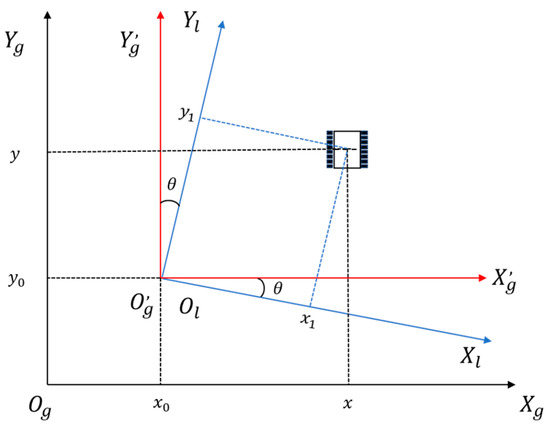
Figure 5.
Planar coordinate system diagram.
First, the laser odometer coordinate system is used as the unified coordinate system, and is the starting position of the autonomous positioning navigation system. The angle between the axis of the laser odometer coordinate system and true north is obtained by receiving the heading angle output from INS as , and then the GNSS navigation plane coordinates after Gaussian projection are transformed by translation to obtain in the laser odometer coordinate system as
By rotating and translating the coordinate system, an accurate description of the laser odometer positioning information, the GNSS positioning information, and the navigation path in the same coordinate system can be obtained. Following the conversion of the coordinate system, the system now articulates the positioning information from both the laser odometer and GNSS, along with the navigation path defined by latitude and longitude, in a unified coordinate framework.
2.2.2. GNSS-Corrected Laser Odometer
The GICP algorithm improves the accuracy and robustness of the registration between point cloud data by considering the position uncertainty of each point. Compared with the traditional ICP algorithm, GICP not only incorporates the Gaussian distribution information of points in the solution process but also uses KD-tree to efficiently search for the nearest point, which greatly accelerates the registration speed. Suppose the source point cloud = and the target point cloud =, which are registered by the estimated transformation matrix . belongs to the special Euclidean group , consists of a rotation matrix and translation vectors, and can be expressed as .
Since real-world measurements include noise, the location of each point cloud is assumed to be the mean of the estimated position that obeys the point. The covariance matrix of the point is the Gaussian distribution of the covariance. and are the mean values of the source point cloud and the target point cloud , respectively. and are the covariance matrices of the source point cloud and the target point cloud , respectively. The source point cloud and the target point cloud are the Gaussian distribution:
The alignment error for each pair of corresponding points can be obtained as
Since are Gaussian distributions independent of each other, then also belongs to a Gaussian distribution:
The iterative calculation of is obtained by the maximum likelihood estimation (MLE) method:
where the residual error is defined as
The GICP algorithm has a wider range of applications than the classical ICP algorithm, and the GICP alignment is better than the ICP in terms of matching speed and accuracy [28]. Therefore, this paper chooses the algorithm based on GICP matching for point cloud alignment. The structure of the laser odometer workflow is shown in Figure 6.
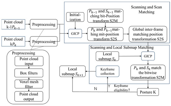
Figure 6.
Laser odometer structure.
After the work described above, we obtained descriptions of GNSS and LiDAR positioning information under a unified coordinate system. In actual use of the LiDAR odometry based on generalized iterative closest point (GICP), we discovered that although its cumulative error is smaller compared to INS, it can still lead to shifts in positioning information over long periods of use. This shift phenomenon is especially noticeable when changing rows, as illustrated in Figure 7a. To enhance the navigation accuracy of the LiDAR odometer in the orchard, we integrate the GNSS positioning information after coordinate alignment to correct and initialize the LiDAR odometer at the end of each row. After reaching the next transverse end of the field, initialization is stopped, and the current frame is used as the initial frame, taking the GNSS output at this moment as the pose information for the initial frame. Then, the keyframes in the stored keyframe library are cleared to eliminate accumulated errors. The effect of the GNSS-corrected LiDAR odometer is shown in Figure 7b.
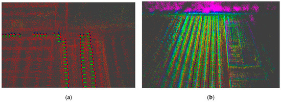
Figure 7.
The laser odometer usage effect diagram. (a) The original laser odometer usage effect; (b) the laser odometer usage effect after GNSS revision.
2.2.3. GNSS-LiDAR Orchard Positioning Scheme Based on Dynamic Switching
To meet the navigation needs of the orchard environment, we utilize the ROS system to subscribe to the GNSS STATUS topic. Based on the assessment of GNSS signal status, we propose a method for dynamically switching between GNSS-LiDAR positioning modes. Figure 8 is a schematic diagram of the work performed by the orchard robotic vehicle. In this diagram, the green areas represent the end of the field, where there is no overhead cover, and the satellite differential signals are good. The yellow areas represent the working areas between the rows of trees, and the black areas are where satellite signals are obstructed. During operation, the orchard robotic vehicle dynamically switches between odometer positioning information and RTK-GNSS positioning information, based on the GNSS signal status. In the green areas, the orchard robotic vehicle navigates using RTK-GNSS positioning information. In the black areas, it determines the switch to laser odometer positioning mode by assessing GNSS signal status. Upon exiting such areas, it switches back to RTK-GNSS positioning mode.
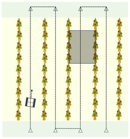
Figure 8.
Schematic diagram of orchard robotic vehicle operation.
2.3. Path-Tracking Control System
2.3.1. Kinematic Model of Robotic Vehicle
To adapt to the complex, uneven, and soft soil ground in the orchard, the robotic vehicle adopts a track structure for its chassis. This structure has a large contact area with the ground, providing greater friction and stronger off-road performance compared to wheel drive, making it more suitable for the orchard environment. The chassis used in this study is based on the principle of differential motion, whereby steering is achieved by controlling the speed difference between the left and right tracks. We assume that the surface of the orchard roads is approximately a two-dimensional plane, and the mass of the mobile platform is uniformly distributed. Its center of mass is located on the geometric longitudinal symmetry line, and it will not deflect or slip during driving. Based on this, a differential drive kinematic model is established.
The robot kinematics model is shown in Figure 9. The point is the center of mass of the moving platform, XOY is the world coordinate system, and is the robot coordinate system. The forward motion direction is the positive direction of the y-axis, the right motion direction is the positive direction of the x-axis, and the z-axis is perpendicular to the paper surface outward. At this time, the position of the robot is represented by the vector , which serves as the reference coordinate point of the moving platform in the orchard. is the center of rotation center of mass; v is the linear velocity of the center of mass; is the turning radius of the center of mass; , are the linear velocities of the left and right driving wheels; is the angular velocity of the center of mass with respect to the rotational center ; and is the distance between the centers of the two tracks.
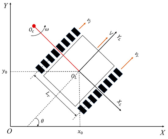
Figure 9.
Kinematic modeling of tracked differential movement.
The linear velocity of the orchard moving platform can be expressed as
The angular velocity of the orchard moving platform can be expressed as
The derivative of the positional state of the orchard moving platform is
According to Equations (20) and (21), are, respectively,
The above equation shows that controlling the rotational speed of the tracks on both sides of the robotic vehicle can realize the control of its steering and driving speed, which can be obtained by discretization:
In summary, it can be seen that by controlling the rotational speed of the tracks on both sides of the robot, it is possible to control the robot’s steering and straight-line travel.
2.3.2. PID-Based Path-Tracking Algorithm
Due to the uneven ground of the orchard and the soft soil, the mobile platform of the orchard often deflects and slips during the walking process, causing it to deviate from the preset navigation path. The PID control algorithm is an important part of classical control theory and has been widely used in practical engineering [29], and we use it to implement path-tracking control.
The essence of a PID controller is a linear controller. In the PID control system, the selection of PID controller parameters , , can significantly affect the effectiveness of the system. Continuous PID algorithm prototype formula:
where is the PID controller output regulation, is the proportionality coefficient, is the real value and the set value of the error, is the integral time constant, and is the differential time constant.
Since the industrial control machine cannot directly use the continuous PID prototype function, the algorithm is discretized as follows:
where , , correspond to the three parameters , , and in the PID controller, is the error between the real value and the set value at n moments, and T is the sampling period.
The PID controller studied in this paper takes the heading deviation and lateral deviation d between the navigation process of the robotic vehicle in the orchard and the set navigation line as inputs, and the left and right wheel rotational speeds of the mobile chassis as outputs. The control principle is shown in Figure 10, and the control model is as follows:
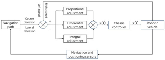
Figure 10.
PID navigation control model.
This can be obtained by combining the differential robot model above:
The sampling time was set to 250 milliseconds, and the path-tracking speed to v = 0.25 m/s. Through testing, it was determined that when = 59.6, , , and , the system exhibits the best stability and fastest response time. The simulation results of the PID control performance under the selected parameters are shown in Figure 11. The controller used in this paper has a rise time of no more than 1 s, a lateral deviation overshoot of no more than 0.1 m, a course deviation overshoot of no more than 0.2 rad, a settling time of no more than 2 s, and a steady-state error of zero. These characteristics meet the fundamental requirements of PID control.
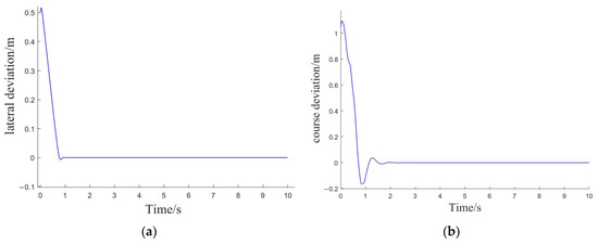
Figure 11.
Simulation results of PID control performance. (a) Simulation results of lateral deviation over time; (b) simulation results of course deviation over time.
3. Results
3.1. Experiment Setting
To verify the performance of the orchard navigation system proposed in this paper, tests on its path-tracking and positioning functions were conducted in an apple orchard in Beijing City, as shown in Figure 12. Five rows of apple trees were selected in the experimental area, spaced approximately 3.5 m apart, with each row being about 95 m long, and the orchard floor was covered in weeds. The robot vehicle walked through the rows of apple trees, covering a total distance of about 360 m. During the test, a dynamic switching GNSS/INS-LiDAR positioning mode was used within the rows of trees, while the GNSS/INS positioning method was employed at the row ends. Given that the positioning information error obtained by the GNSS/INS navigation system under good signal conditions is equal to or less than 1.5 cm, this experiment used it as the actual path trajectory during the orchard traversal process.
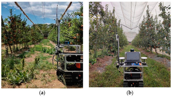
Figure 12.
Experimental scenario orchard environment. (a) Unshaded orchard environment; (b) orchard environment under bird-proof netting.
3.2. Navigation Test with Unobstructed GNSS
In the experimental orchard area without anti-bird nets, the road between the rows of apple trees has no overhead obstructions. This condition allows for a strong satellite differential signal, enabling the autonomous navigation test for the orchard’s robotic vehicle. Given the robust satellite differential signal, the system relies solely on the GNSS/INS system’s positioning information for path tracking. The walking trajectory during navigation is shown in Figure 13, and the lateral deviation value of the real walking trajectory from the preset navigation path is shown in Figure 14. Due to the uneven ground of the orchard, and because the robotic vehicle used in the test is small and prone to side-slip, the lateral deviation value fluctuates greatly in the figure. The test indicates that the maximum path-tracking lateral error does not exceed 0.35 m, and the average path-tracking lateral error does not exceed 0.1 m. The standard deviation of the lateral error is 0.076 and the root mean square error (RMSE) is 0.016 m.
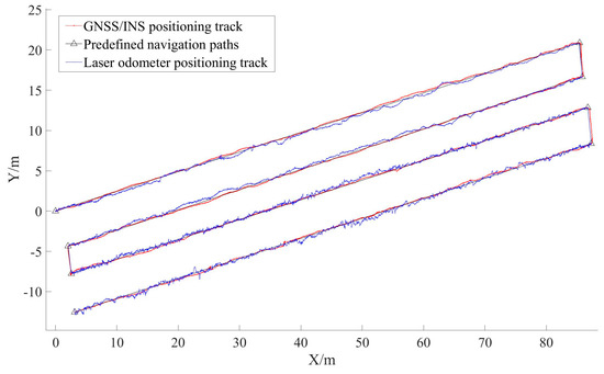
Figure 13.
Localization trajectories of the robotic vehicle in linear navigation experiments in an orchard environment.
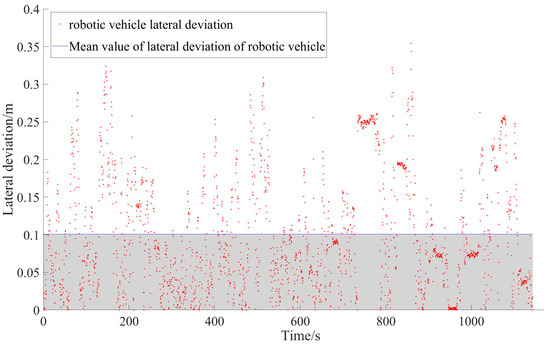
Figure 14.
Lateral deviation of navigation trajectories of the robotic vehicle moving along the tree lines with unobstructed GNSS.
3.3. Navigation Test with Intermittent GNSS Dropout
An anti-bird net was laid over a part of the road between the third and fourth rows of apple trees in the orchard experimental area to test the effect of satellite differential signal blocking. The positioning trajectory during navigation is shown in Figure 15. Figure 16 shows the positioning deviation of the laser odometer and the GNSS/INS positioning deviation of the occluded part of the satellite differential signal. The positioning deviations of the laser odometer and the GNSS/INS under obstruction conditions are shown in Table 1. The average positioning deviation of the laser odometer is 0.14 m, the maximum positioning deviation is 0.62 m, the standard deviation is 0.115, and the RMSE is 0.0328 m. When the satellite differential signal is obstructed, the average positioning deviation of the GNSS/INS positioning system is 1.24 m, the maximum positioning deviation is 2.23 m, the standard deviation is 0.6927, and the RMSE is 2.0195 m. When the satellite signal is blocked, the positioning accuracy of the laser odometer and the fluctuation of positioning error are better than that of the GNSS/INS navigation and positioning system.
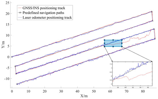
Figure 15.
Localization trajectories of the robotic vehicle moving along the tree lines with intermittent GNSS dropout.
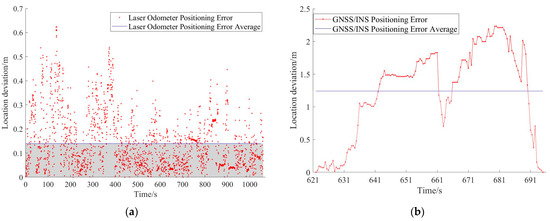
Figure 16.
Positioning bias of robotic vehicle in orchard environment: (a) positioning error of laser odometer; (b) positioning error of GNSS/INS in blocked section of satellite signal.

Table 1.
Comparison of positioning deviation between laser odometer and GNSS/INS under occlusive conditions.
4. Discussion
The satellite signal enables RTK differential positioning without barriers, achieving a GNSS/INS navigation accuracy within 1.5 cm. This accuracy serves as the baseline for the robotic vehicle’s path trajectory during autonomous navigation. Field tests show that with satellite signal blockage, GNSS/INS positioning records an average error of about 1.24 m and a maximum error of roughly 2.23 m, alongside a standard deviation of 0.69 and an RMSE of 2.02 m. Conversely, the laser odometer’s average error remains below 0.14 m, with the maximum deviation not exceeding 0.63 m, a standard deviation of 0.16, and an RMSE of 0.03 m. By the fusion of the laser positioning information, the problem of intermittent loss of satellite positioning signals in the complex environment of the orchard is effectively overcome. Although the positioning error fluctuates greatly, it can be used as the basis for the robotic vehicle’s navigation and positioning when the satellite signal is lost or blocked. Its positioning accuracy is acceptable for orchard spraying, weeding, transportation, and other uses of mechanical mobile platforms. The results are expected to improve the navigation capability of autonomous operating equipment in orchards.
5. Conclusions
To mitigate the issue of signal blockage by dense orchard canopies causing significant drops in satellite navigation system accuracy, this study introduces a loosely coupled laser odometer and GNSS/INS system for robotic vehicles in orchards. The approach includes creating the vehicle’s kinematic model, developing a PID-based path-tracking algorithm, planning paths tailored to orchard terrain, and executing navigation trials. Results indicate that with the robotic vehicle moving at 0.35 m/s, the peak tracking error stays below 0.35 m, the mean absolute error remains under 0.1 m, with a standard deviation close to 0.078, and an RMSE under 0.017 m. The autonomous navigation and control system adopted by the robotic vehicle meets the requirements of autonomous navigation of orchard robots. It improves the navigation accuracy in the partially obstructed orchard environment and improves the performance of the navigation system. When satellite signals are obstructed, laser odometry becomes the standard for navigation and positioning. Compared to the GNSS/INS method, this approach reduces the maximum and average positioning deviations by 1.6 m and 1.1 m, respectively. This effectively enhances navigation stability and positioning accuracy under conditions of blocked satellite signals, overcoming the challenges of self-positioning in environments where satellite signal interruptions occur. The disadvantage is that the positioning error of the laser odometer fluctuates greatly, which still needs to be further optimized and improved.
Author Contributions
Conceptualization, Q.F. and Y.L.; methodology, Y.L.; software, Y.L.; validation, Q.F.; formal analysis, Y.L.; investigation, Y.S.; resources, Q.F.; data curation, J.S.; writing—original draft preparation, Y.L.; writing—review and editing, Y.L. and Q.F.; supervision, C.J.; project administration, C.J.; funding acquisition, Q.F. All authors have read and agreed to the published version of the manuscript.
Funding
This work was sponsored by the Science and Technology Cooperation Project of Xinjiang Production and Construction Corps (2022BC007), BAAFS Innovation Capacity Building Project (KJCX20240502).
Institutional Review Board Statement
Not applicable.
Informed Consent Statement
Not applicable.
Data Availability Statement
The original contributions presented in the study are included in the article, further inquiries can be directed to the corresponding author.
Acknowledgments
We wish to thank the above foundations for their support.
Conflicts of Interest
The authors declare that this study received funding from Science and Technology Cooperation Project of Xinjiang Production and Construction Corps. The funder was not involved in the study design, collection, analysis, interpretation of data, the writing of this article or the decision to submit it for publication.
References
- Dou, J.H.; Chen, Z.Y.; Zhai, C.Y.; Zou, W.; Song, J.; Feng, F.; Zhang, Y.L.; Wang, X. Research Progress on Autonomous Navigation Technology for Orchard Intelligent Equipment. Trans. Chin. Soc. Agric. Mach 2024, 68, 1–25. [Google Scholar]
- Zhao, Y.; Xiao, H.; Mei, S.; Song, Z.; Ding, W.; Jing, Y. Current status and development strategies of orchard mechanization production in China. J. China Agric. Univ. 2017, 22, 116–127. [Google Scholar]
- Liu, J. Research Progress Analysis of Robotic Harvesting Technologies in Greenhouse. Trans. Chin. Soc. Agric. Mach 2017, 48, 1–18. [Google Scholar]
- Vougioukas, S.; Spanomitros, Y.; Slaughter, D. Dispatching and Routing of Robotic Crop-transport Aids for Fruit Pickers using Mixed Integer Programming. In Proceedings of the American Society of Agricultural and Biological Engineers, Dallas, TX, USA, 29 July–1 August 2012; pp. 3423–3432. [Google Scholar]
- Yin, X.; Wang, Y.; Chen, Y.; Jin, C.; Du, J. Development of autonomous navigation controller for agricultural vehicles. Int. J. Agric. Biol. Eng. 2020, 13, 70–76. [Google Scholar] [CrossRef]
- Nørremark, M.; Griepentrog, H.W.; Nielsen, J.; Søgaard, H.T. The development and assessment of the accuracy of an autonomous GPS-based system for intra-row mechanical weed control in row crops. Biosyst. Eng. 2008, 101, 396–410. [Google Scholar] [CrossRef]
- Jilek, T. Autonomous field measurement in outdoor areas using a mobile robot with RTK GNSS. IFAC IEEE Conf. Program. Devices Embed. Syst. 2015, 48, 480–485. [Google Scholar] [CrossRef]
- Han, J.H.; Park, C.H.; Park, Y.J.; Kwon, J.H. Preliminary Results of the Development of a Single Frequency GNSS RTK-Based Autonomous Driving System for a Speed Sprayer. J. Sens. 2019, 2, 1–9. [Google Scholar] [CrossRef]
- Fresk, E.; Nikolakopoulos, G.; Gustafsson, T. A Generalized Reduced-Complexity Inertial Navigation System for Unmanned Aerial Vehicles. IEEE Trans. Control Syst. Technol. 2016, 25, 192–207. [Google Scholar] [CrossRef]
- Hwang, S.Y.; Lee, J.M. Estimation of Attitude and Position of Moving Objects Using Multi-filtered Inertial Navigation System. Trans. Korean Inst. Electr. Eng. 2011, 60, S446–S452. [Google Scholar]
- Hu, L.; Wang, Z.; Wang, P.; He, J.; Jiao, J.; Wang, C.; Li, M. Agricultural robot positioning system based on laser sensing. Trans. CSAE 2023, 39, 1–7. [Google Scholar]
- Freitas, G.; Zhang, J.; Hamner, B.; Bergerman, M.; Kantor, G. A low-cost, practical localization system for agricultural vehicles. In Proceedings of the Intelligent Robotics and Applications: 5th International Conference, ICIRA 2012, Montreal, QC, Canada, 3–5 October 2012; pp. 365–375. [Google Scholar]
- Zhou, J.; Hu, C. Inter-row Localization Method for Agricultural Robot Working in Close Planting Orchard. Trans. Chin. Soc. Agric. Mach. 2015, 46, 22–28. [Google Scholar]
- Shalal, N.; Low, T.; McCarthy, C.; Hancock, C. Orchard mapping and mobile robot localisation using on-board camera and laser scanner data fusion–Part B: Mapping and localisation. Comput. Electron. Agric. 2015, 119, 267–278. [Google Scholar] [CrossRef]
- Zhang, S.; Guo, C.; Gao, Z.; Sugirbay, A.; Chen, J.; Chen, Y. Research on 2D Laser Automatic Navigation Control for Standardized Orchard. Appl. Sci. 2020, 10, 2763. [Google Scholar] [CrossRef]
- Ma, Y.; Zhang, W.; Qureshi, W.S.; Gao, C.; Zhang, C.; Li, W. Autonomous navigation for a wolfberry picking robot using visual cues and fuzzy control. Inf. Process. Agric 2021, 8, 15–26. [Google Scholar] [CrossRef]
- Huang, Y.; Fu, J.; Xu, S.; Han, T.; Liu, Y. Research on Integrated Navigation System of Agricultural Machinery Based on RTK-BDS/INS. Agriculture 2022, 12, 1169. [Google Scholar] [CrossRef]
- Sun, B.; Yeary, M.; Sigmarsson, H.H.; Mcdaniel, J.W. Fine resolution position estimation using Kalman Filtering. In Proceedings of the 2019 IEEE International Instrumentation and Measurement Technology Conference (I2MTC), Auckland, New Zealand, 20–23 May 2019; pp. 1–5. [Google Scholar]
- Qian, C.; Liu, H.; Tang, J.; Chen, Y.; Kaartinen, H.; Kukko, A.; Zhu, L.; Liang, X.; Chen, L.; Hyyppä, J. An Integrated GNSS/INS/LiDAR-SLAM Positioning Method for Highly Accurate Forest Stem Mapping. Remote Sens. 2017, 9, 3. [Google Scholar] [CrossRef]
- Chiang, K.W.; Duong, T.T.; Liao, J.K. The Performance Analysis of a Real-Time Integrated INS/GPS Vehicle Navigation System with Abnormal GPS Measurement Elimination. Sensors 2013, 13, 10599–10622. [Google Scholar] [CrossRef] [PubMed]
- Ball, D.; Upcroft, B.; Wyeth, G.; Corke, P.; English, A.; Ross, P.; Patten, T.; Fitch, R.; Sukkarieh, S.; Bate, A. Vision-based obstacle detection and navigation for an agricultural robot. J. Field Robot. 2016, 33, 1107–1130. [Google Scholar] [CrossRef]
- Zuo, Z.; Yang, B.; Li, Z.; Zhang, T. A GNSS/IMU/vision ultra-tightly integrated navigation system for low altitude aircraft. IEEE Sens. J. 2022, 22, 11857. [Google Scholar] [CrossRef]
- Chu, T.; Guo, N.; Backén, S.; Akos, D. Monocular Camera/IMU/GNSS Integration for Ground Vehicle Navigation in Challenging GNSS Environments. Sensors 2012, 12, 3162–3185. [Google Scholar] [CrossRef]
- Shamsudin, A.U.; Ohno, K.; Hamada, R.; Kojima, S.; Westfechtel, T.; Suzuki, T.; Okada1, Y.; Tadokoro, S.; Fujita, J.; Amano, H. Consistent map building in petrochemical complexes for firefighter robots using SLAM based on GPS and LIDAR. Robomech 2018, 5, 1–13. [Google Scholar]
- Jiang, W.; Yu, Y.; Zong, K.; Cai, B.; Rizos, C.; Wang, J.; Liu, D.; Shangguan, W. A Seamless Train Positioning System Using a Lidar-Aided Hybrid Integration Methodology. IEEE Trans. Veh. Technol 2021, 70, 6371–6384. [Google Scholar] [CrossRef]
- Elamin, A.; Abdelaziz, N.; El-Rabbany, A. A GNSS/INS/LiDAR Integration Scheme for UAV-Based Navigation in GNSS-Challenging Environments. Sensors 2022, 22, 9908. [Google Scholar] [CrossRef] [PubMed]
- Segal, A.; Haehnel, D.; Thrun, S. Generalized-ICP. In Proceedings of the Robotics: Science and Systems V, University of Washington, Seattle, DC, USA, 28 June–1 July 2009. [Google Scholar]
- Hyoseok, K.; Chang-Woo, P.; Chang-Ho, H. Alternative identification of wheeled mobile robots with skidding and slipping. Int. J. Control. Autom. Syst. 2016, 14, 1055–1062. [Google Scholar]
- Yu, S.H.; Hyun, C.H.; Kang, H.S. Robust dynamic surface tracking control for uncertain wheeled mobile robot with skidding and slipping. In Proceedings of the IEEE International Conference on Control and Robotics Engineering, Singapore, 2–4 April 2016; IEEE: Piscataway, NJ, USA, 2016; pp. 1–4. [Google Scholar]
Disclaimer/Publisher’s Note: The statements, opinions and data contained in all publications are solely those of the individual author(s) and contributor(s) and not of MDPI and/or the editor(s). MDPI and/or the editor(s) disclaim responsibility for any injury to people or property resulting from any ideas, methods, instructions or products referred to in the content. |
© 2024 by the authors. Licensee MDPI, Basel, Switzerland. This article is an open access article distributed under the terms and conditions of the Creative Commons Attribution (CC BY) license (https://creativecommons.org/licenses/by/4.0/).