


Trajectory Planning and Singularity Avoidance Algorithm for Robotic Arm Obstacle Avoidance Based on an Improved Fast Marching Tree

Abstract
1. Introduction
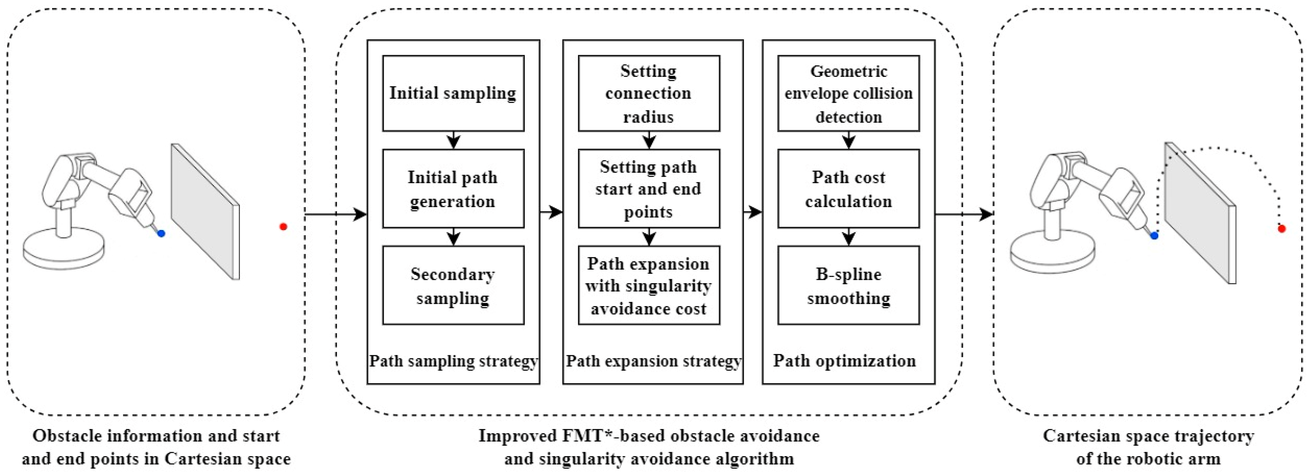
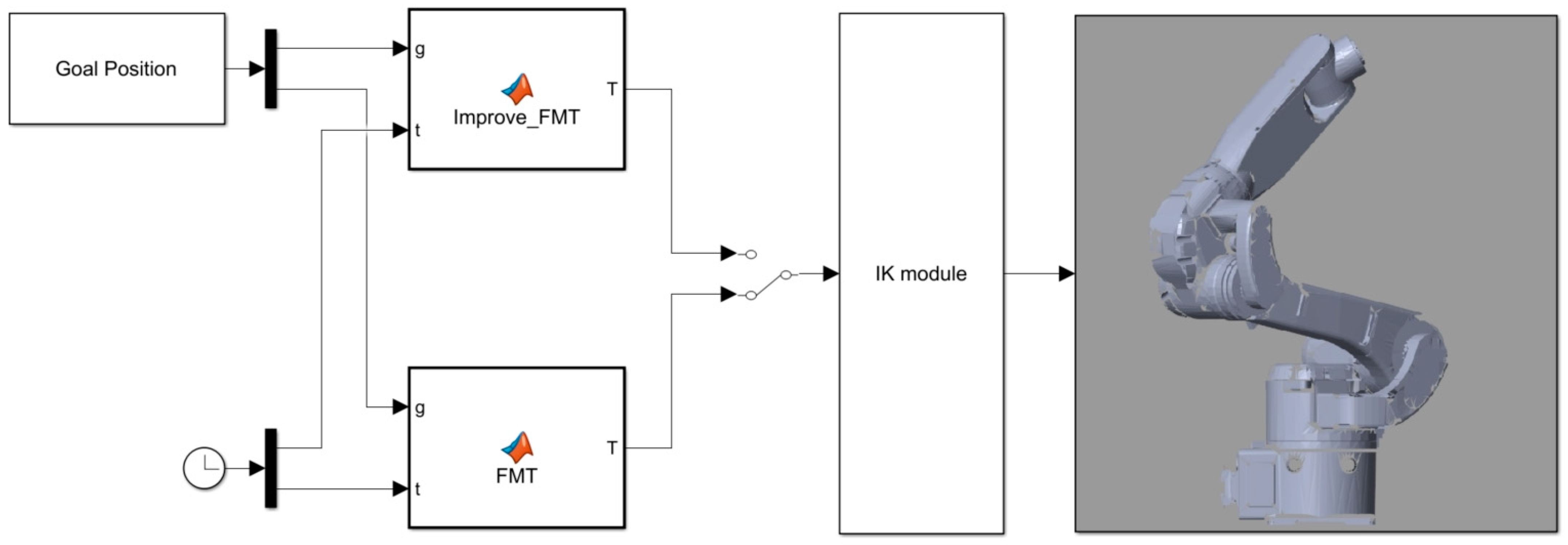
2. Methods
| Algorithm 1 Improved FMT* |
| Data: Xfree, Xinit, Xgoal, n, R1, R2 |
| Result: BestPath |
| 1: π←STANDARD FMT*(Xfree, xinit, xgoal, n, R1) |
| 2: V←SECONDARY SAMPLING(Xfree, π, n, width) |
| 3: II←SECONDARY EXPANSION(V, xinit, xgoal, R2) |
| 4: ) |
2.1. Principles of the FMT* Algorithm
| Algorithm 2 Standard Fast Marching Tree (FMT*) |
| 1: function STANDARD FMT*(Xfree, xinit, xgoal, n, R1) |
| 2: success = FALSE |
| 3: stop_expansion = FALSE |
| 4: S←xinit ∪ xgoal ∪ PSEUDO RANDOM SAMPLING(Xfree, n) |
| 5: T←INITIALIZE(S, xinit) |
| 6: z→xinit |
| 7: while (stop_expansion = FALSE and success = FALSE) do |
| 8: {T, z, success, stop_expansion}←EXPAND(Xfree, xinit, xgoal, R1) |
| 9: if (success = TRUE) then |
| 10: π←PATH(xinit, xgoal, T) |
| 11: else |
| 12: π→Ø |
| 13: end if |
| 14: end while |
| 15: return π, T |
| 16: end function |
2.2. Improved Path Point Sampling Strategy
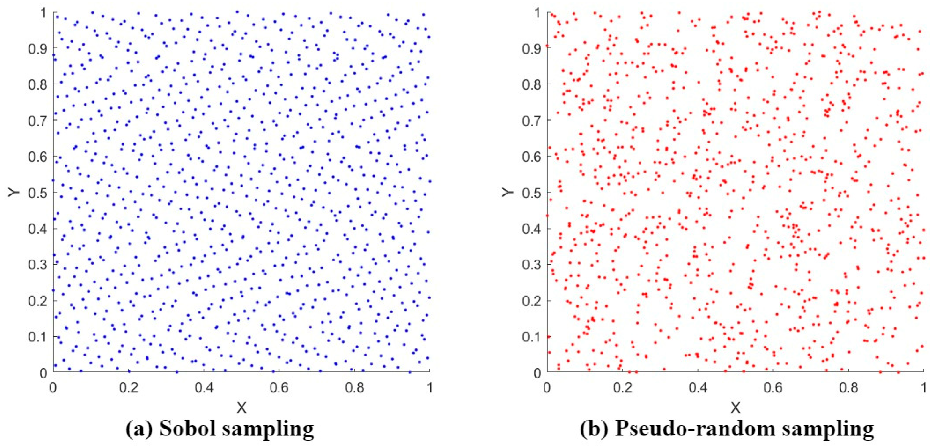
2.2.1. Initial Sampling
2.2.2. Secondary Sampling
| Algorithm 3 Secondary Sampling |
| 1: function SECONDARY SAMPLING(Xfree, π, n, width) |
| 2: path←INITAL PATH SEGMENTATION(π)//Segmenting the path formed by standard FMT* |
| 3: path_num←PATH SORT(π) //sort the path segments and return the total number |
| 4: CLEAR(Xfree) //clearing initial sampling points |
| 5: i = 0 |
| 6: while (i < path_num) do |
| 7: XPath←RESIZE PATH WIDTH(width)//resize the width of the initial sampling paths |
| 8: XPath ∩ Xfree = XSample |
| 9: Secondary_Point←SOBOL SAMPLING(XSample, point_num) |
| 10: if OUTSIDE OBSTACLE(SecondaryPoint) == TRUE then |
| 11: DELETE(SecondaryPoint) |
| 12: else |
| 13: V←APPEND(SecondaryPoint) |
| 14: end if |
| 15: i = i + 1 |
| 16: end while |
| 17: return V |
| 18: end function |
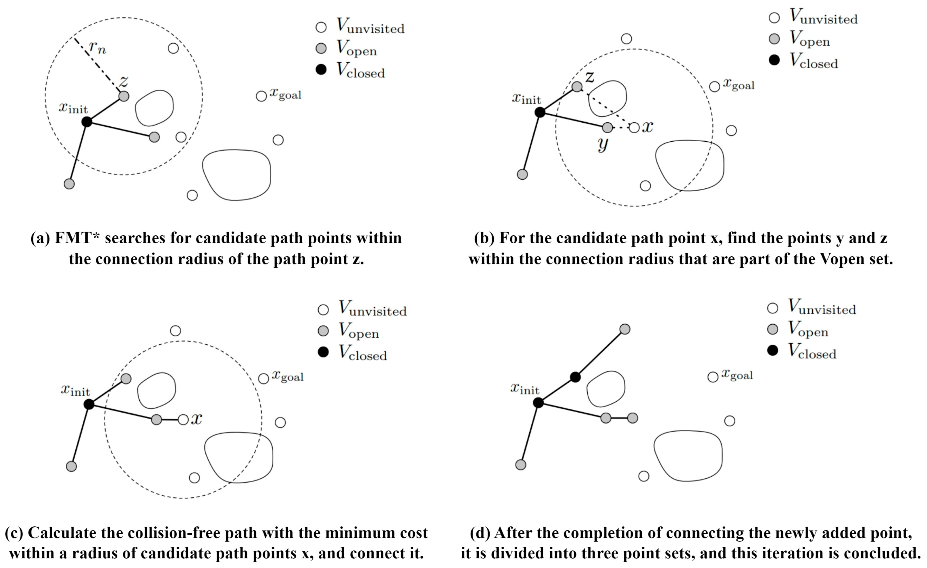
2.3. Path Connection
| Algorithm 4 Secondary Expansion |
| 1: function SECONDARY EXPANSION(V, xinit, xgoal, R2) |
| 2: Vunvisited←V\{xinit} |
| 3: Vopen←{xinit} |
| 4: Vdosed←Ø |
| 5: z←xinit |
| 6: Nz←Near(V\{z}, z, R2) |
| 7: while (z ≠ xgoal) do |
| 8: for x ∈ Nz do |
| 9: Nx←Near(V\{x}) |
| 10: Ny←Nx ∩ Vopen |
| 11: ymin←argminy∈Ny {c(y) + Cost(y, x)} |
| 12: if CollisionFree(ymin, x) then |
| 13: T←T ∪ {(ymin, x)} |
| 14: Vopen,new←Vopen,new ∪ {x} |
| 15: Vunvisited←Vunvisited\{x} |
| 16: c(x) = c(ymin) + cost(ymin, x) + sigcost(x) |
| 17: end if |
| 18: end for |
| 19: Vopen←{Vopen ∪ Vopen,new}\{z} |
| 20: Vclosed←Vclosed ∪ {z} |
| 21: if Vopen = Ø then |
| 22: return stop_expansion |
| 23: end if |
| 24: z←argminy∈Vopen {z} |
| 25: end while |
| , T, success |
| 27: end function |
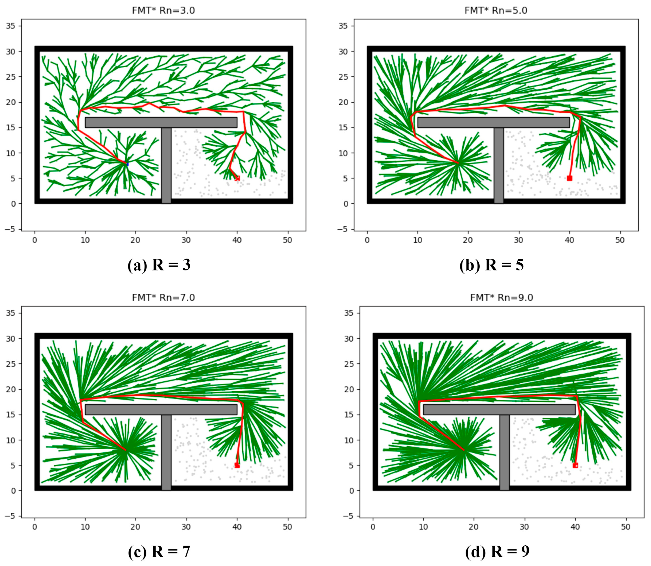
2.3.1. Two-Stage Connection Parameter Settings
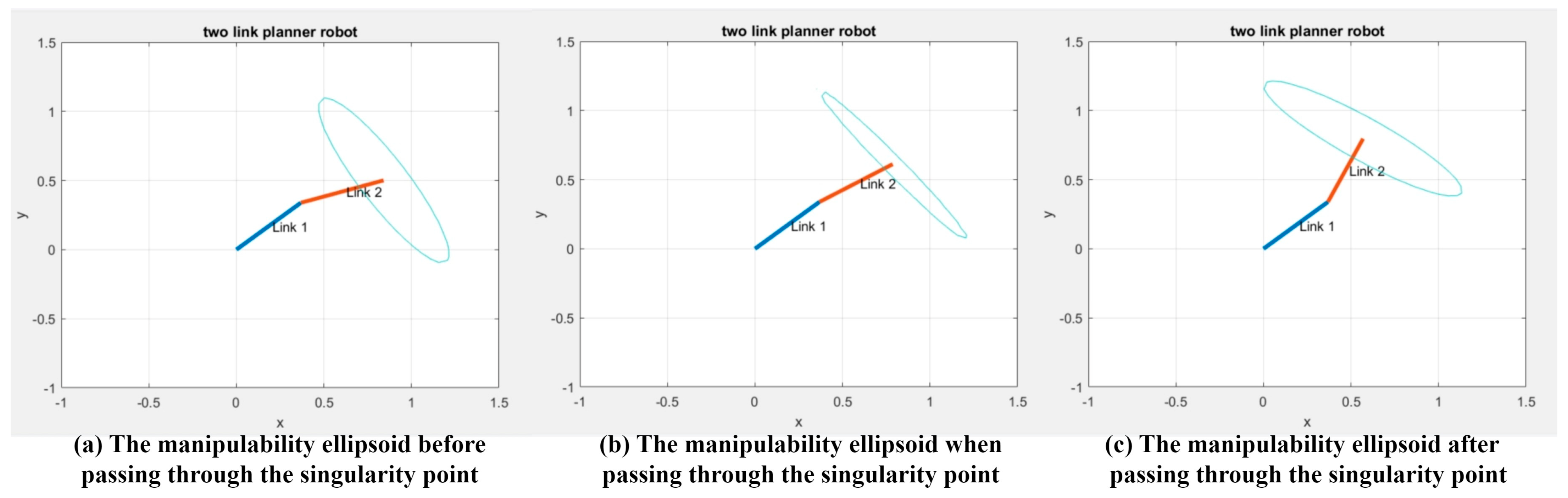
2.3.2. Avoiding Singularities Cost
2.4. Path Optimization
2.4.1. Collision Detection
2.4.2. Path Cost Calculation
2.4.3. Path Smoothing
2.5. Computational Complexity
2.5.1. Time Complexity Analysis
2.5.2. Space Complexity Analysis
3. Experiment and Result
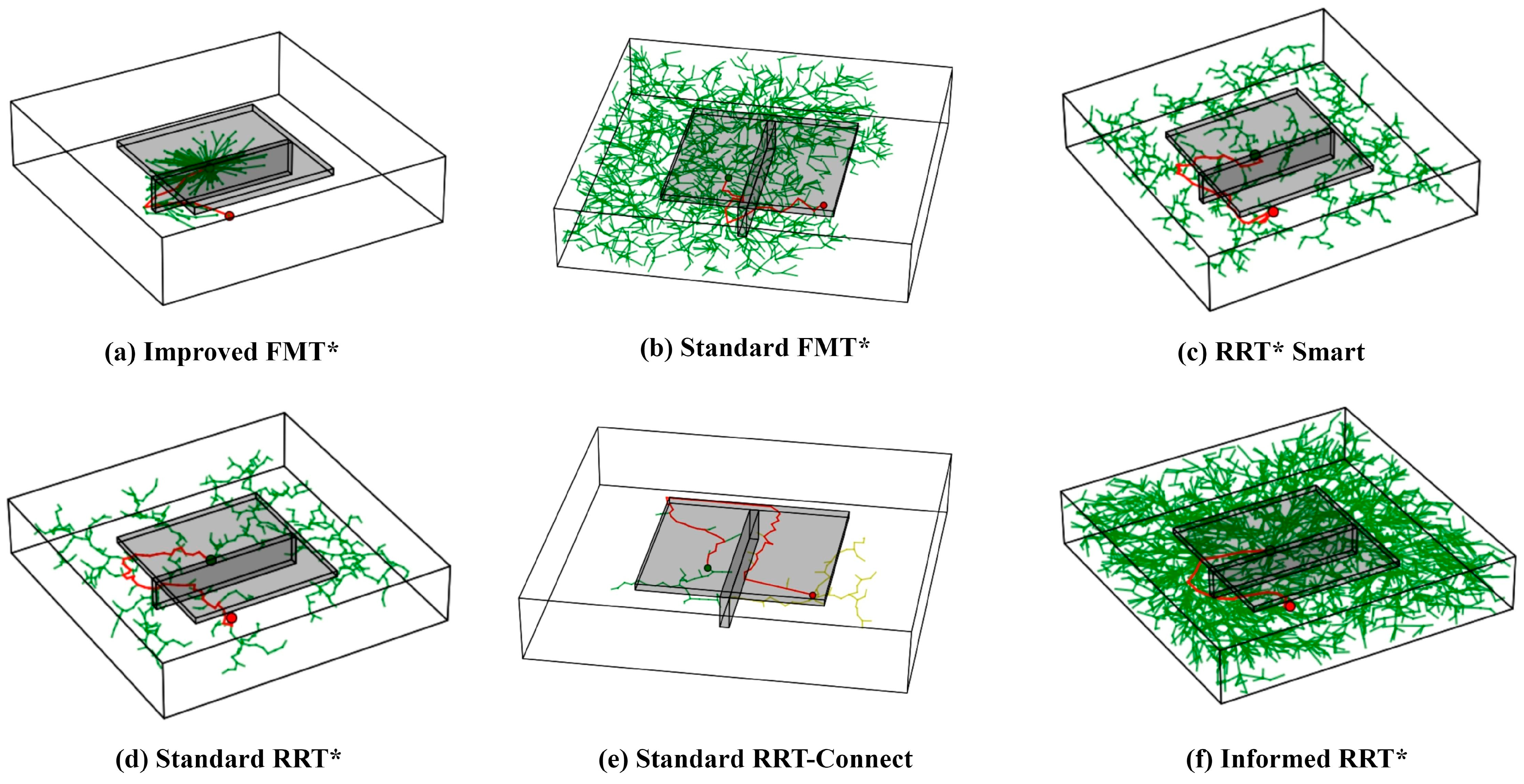
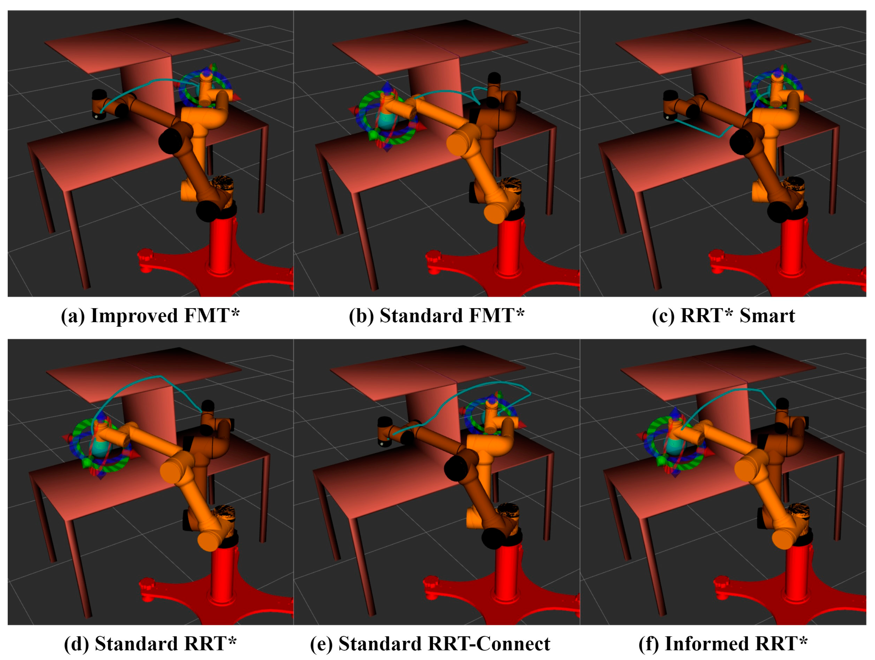
3.1. Obstacle Avoidance Trajectory Planning Simulation Experiment
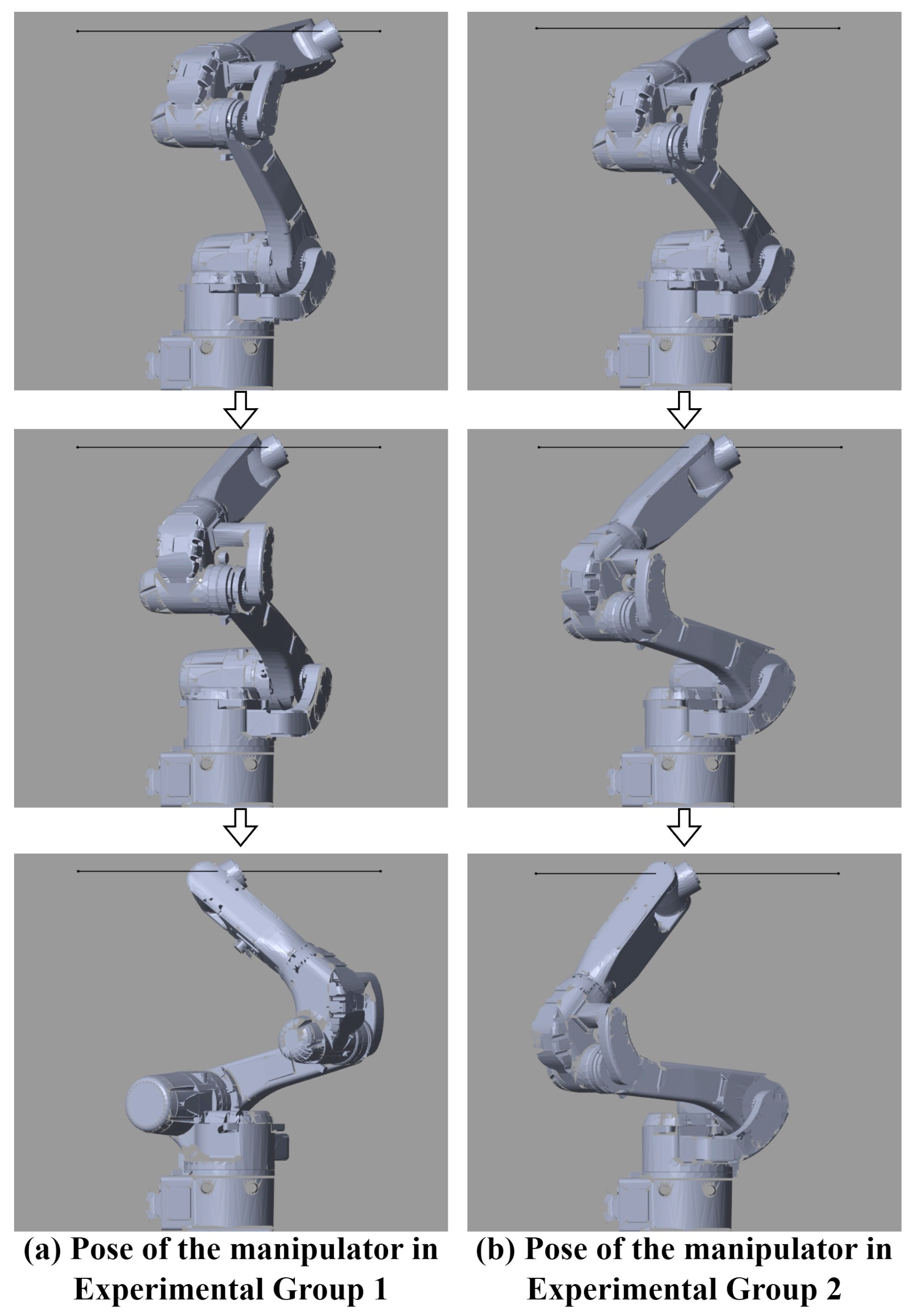
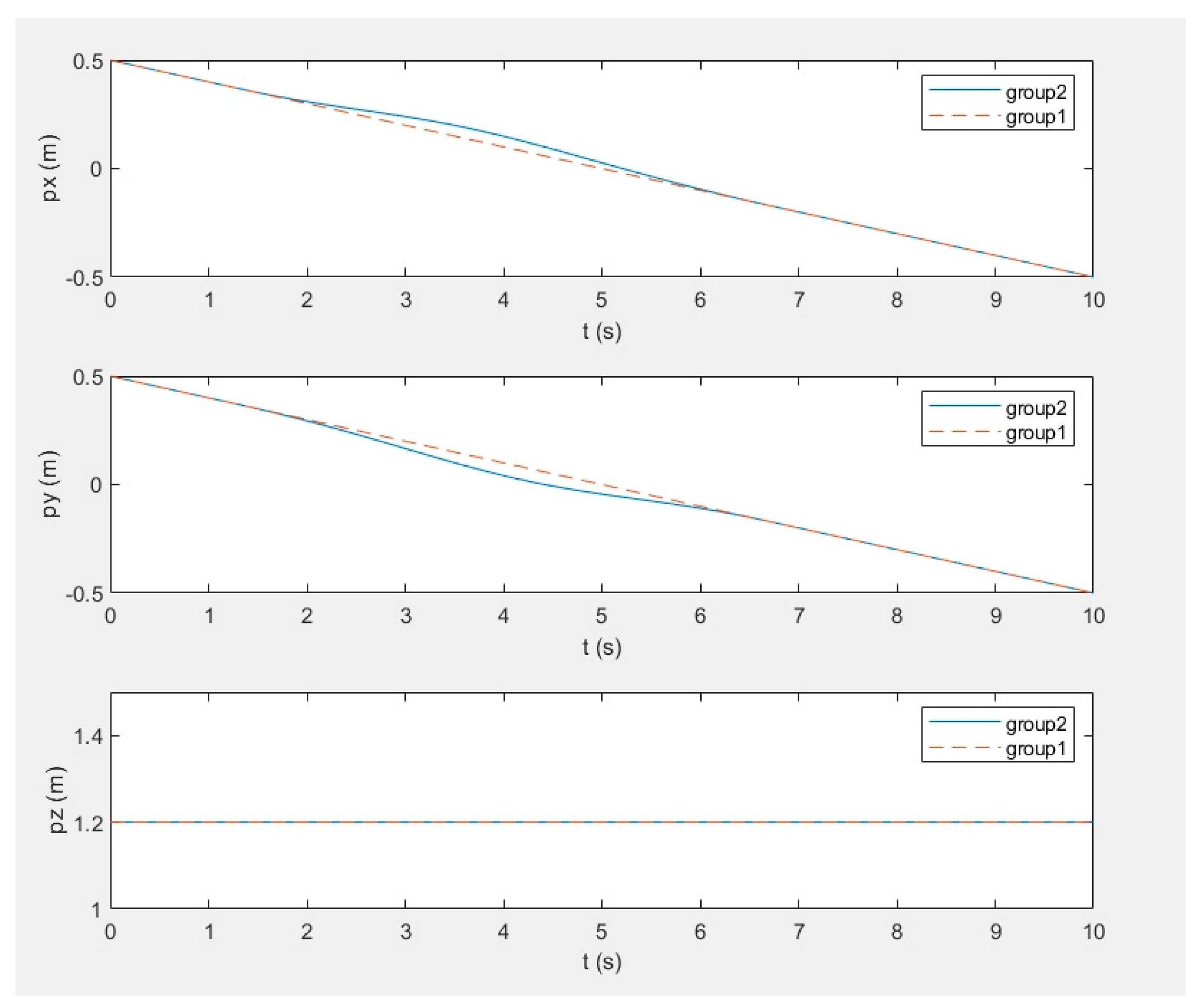
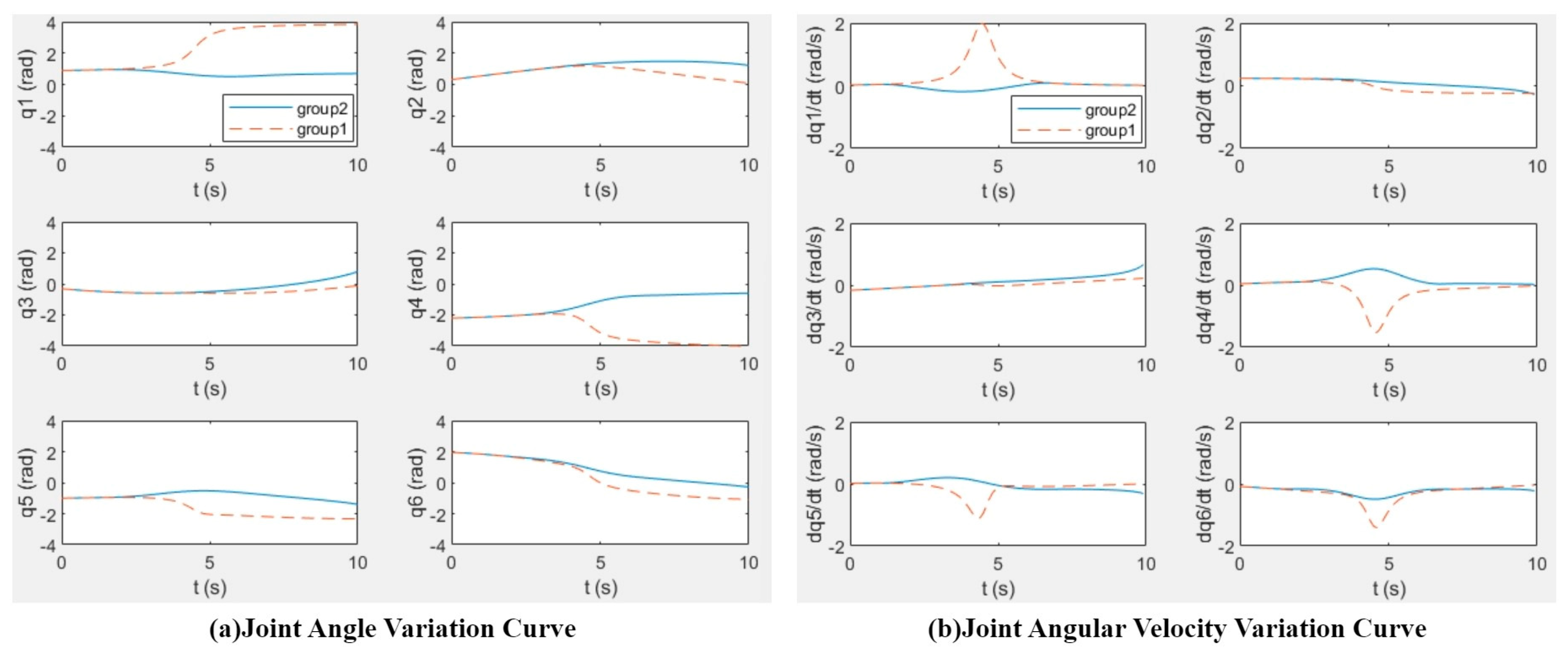
3.2. Singular Point Avoidance Simulation Experiment
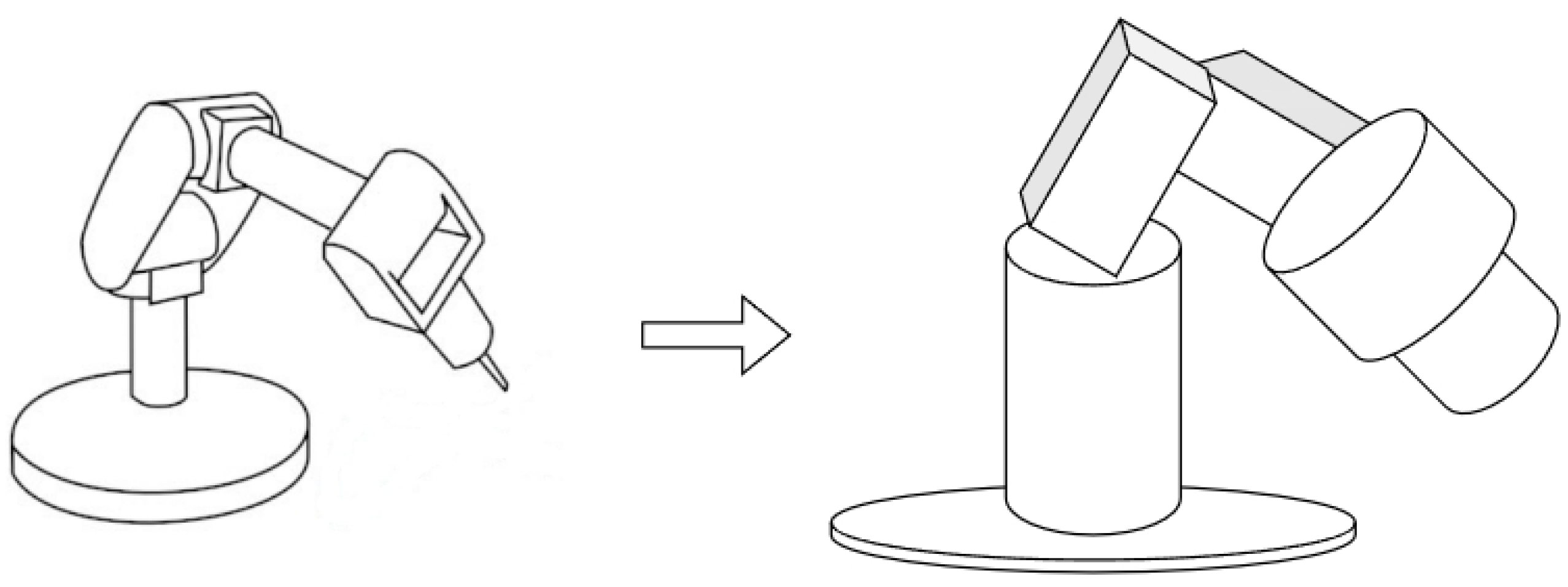
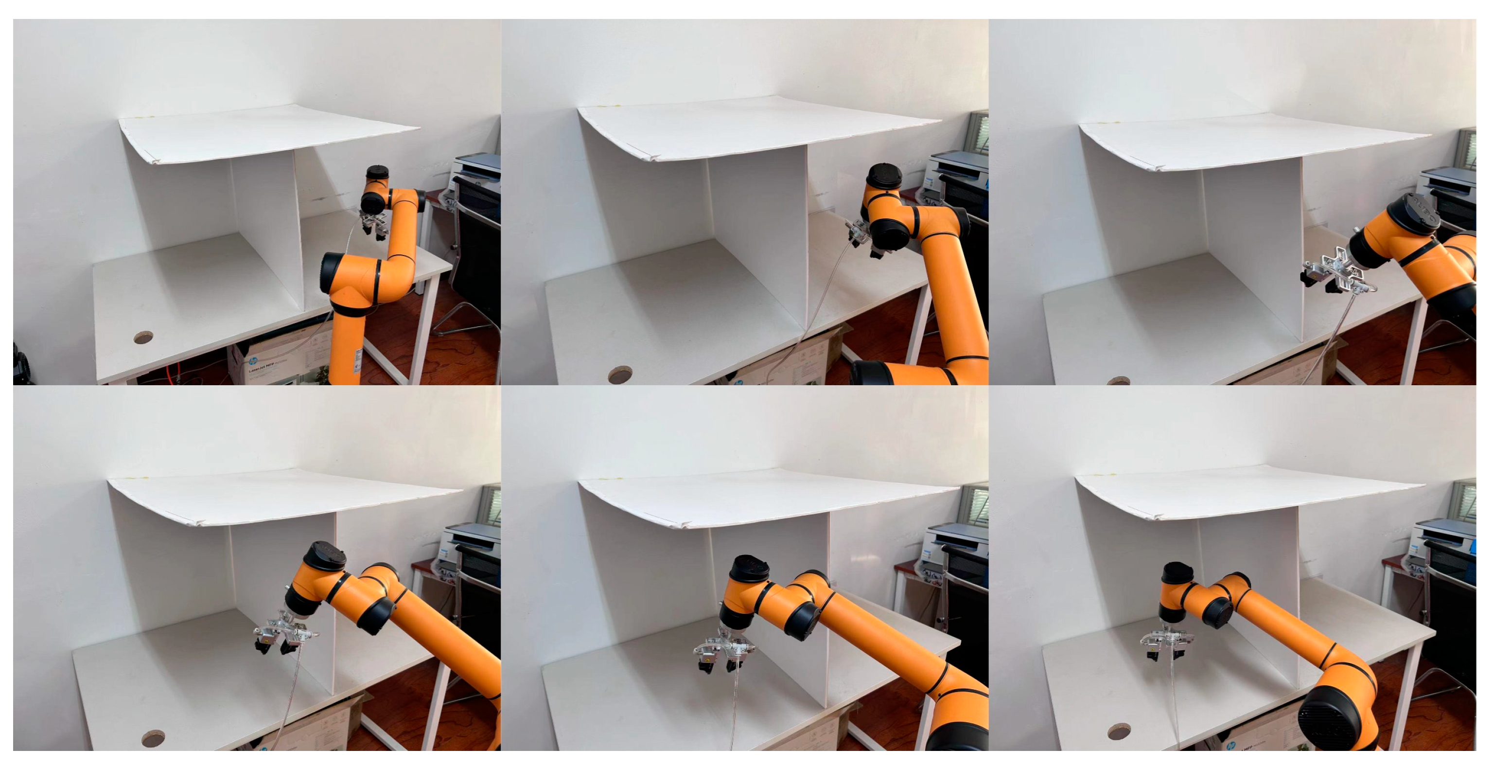
3.3. Robotic Arm Trajectory Planning Experiment in the Real World
4. Discussion
5. Conclusions
Author Contributions
Funding
Institutional Review Board Statement
Informed Consent Statement
Data Availability Statement
Acknowledgments
Conflicts of Interest
References
- Du, Z.-C.; Ouyang, G.-Y.; Xue, J.; Yao, Y.-B. A review on kinematic, workspace, trajectory planning and path planning of hyper-redundant manipulators. In Proceedings of the 2020 10th Institute of Electrical and Electronics Engineers International Conference on Cyber Technology in Automation, Control, and Intelligent Systems (CYBER), Xi’an, China, 10–13 October 2020; pp. 444–449. [Google Scholar] [CrossRef]
- Park, C.; Rabe, F.; Sharma, S.; Scheurer, C.; Zimmermann, U.E.; Manocha, D. Parallel cartesian planning in dynamic environments using constrained trajectory planning. In Proceedings of the 2015 IEEE-RAS 15th International Conference on Humanoid Robots (Humanoids), Seoul, Republic of Korea, 3–5 November 2015; pp. 983–990. [Google Scholar] [CrossRef]
- Khan, A.T.; Li, S.; Kadry, S.; Nam, Y. Control framework for trajectory planning of soft manipulator using optimized RRT algorithm. IEEE Access 2020, 8, 171730–171743. [Google Scholar] [CrossRef]
- Janson, L.; Schmerling, E.; Clark, A.; Pavone, M. Fast marching tree: A fast marching sampling-based method for optimal motion planning in many dimensions. Int. J. Robot. Res. 2015, 34, 883–921. [Google Scholar] [CrossRef]
- Gammell, J.D.; Srinivasa, S.S.; Barfoot, T.D. Batch informed trees (BIT*): Sampling-based optimal planning via the heuristically guided search of implicit random geometric graphs. In Proceedings of the 2015 IEEE International Conference on Robotics and Automation (ICRA), Seattle, WA, USA, 26–30 May 2015; pp. 3067–3074. [Google Scholar] [CrossRef]
- Rybus, T. Point-to-point motion planning of a free-floating space manipulator using the rapidly-exploring random trees (RRT) method. Robotica 2020, 38, 957–982. [Google Scholar] [CrossRef]
- Chen, N.; Zhang, Y.; Cheng, W. Space detumbling robot arm deployment path planning based on Bi-FMT* algorithm. Micromachines 2021, 12, 1231. [Google Scholar] [CrossRef]
- Jin, R.; Rocco, P.; Geng, Y. Cartesian trajectory planning of space robots using a multi-objective optimization. Aerosp. Sci. Technol. 2021, 108, 106360. [Google Scholar] [CrossRef]
- Zhao, H.; Zhang, B.; Yin, X.; Zhang, Z.; Xia, Q.; Zhang, F. Singularity Analysis and Singularity Avoidance Trajectory Planning for Industrial Robots. In Proceedings of the 2021 China Automation Congress (CAC), Beijing, China, 22–24 October 2021; pp. 6164–6169. [Google Scholar] [CrossRef]
- Riboli, M.; Jaccard, M.; Silvestri, M.; Aimi, A.; Malara, C. Collision-free and smooth motion planning of dual-arm Cartesian robot based on B-spline representation. Robot. Auton. Syst. 2023, 170, 104534. [Google Scholar] [CrossRef]
- Ju, F.; Jin, H.; Wang, B.; Zhao, J. A Predictable Obstacle Avoidance Model Based on Geometric Configuration of Redundant Manipulators for Motion Planning. Sensors 2023, 23, 4642. [Google Scholar] [CrossRef] [PubMed]
- Fujii, S.; Pham, Q.-C. Realtime trajectory smoothing with neural nets. In Proceedings of the 2022 International Conference on Robotics and Automation (ICRA), Philadelphia, PA, USA, 23–27 May 2022; pp. 7248–7254. [Google Scholar] [CrossRef]
- Liu, W.; Niu, H.; Mahyuddin, M.N.; Herrmann, G.; Carrasco, J. A model-free deep reinforcement learning approach for robotic manipulators path planning. In Proceedings of the 2021 21st International Conference on Control, Automation and Systems (ICCAS), Jeju Island, Republic of Korea, 12–15 October 2021; pp. 512–517. [Google Scholar] [CrossRef]
- Dai, Y.; Xiang, C.; Zhang, Y.; Jiang, Y.; Qu, W.; Zhang, Q. A Review of spatial robotic arm trajectory planning. Aerospace 2022, 9, 361. [Google Scholar] [CrossRef]
- Liu, Y.; Guo, C.; Weng, Y. Online time-optimal trajectory planning for robotic manipulators using adaptive elite genetic algorithm with singularity avoidance. IEEE Access 2019, 7, 146301–146308. [Google Scholar] [CrossRef]
- Lu, L.; Zhang, L.; Fan, C.; Wang, H. High-order joint-smooth trajectory planning method considering tool-orientation constraints and singularity avoidance for robot surface machining. J. Manuf. Process. 2022, 80, 789–804. [Google Scholar] [CrossRef]
- Beck, F.; Vu, M.N.; Hartl-Nesic, C.; Kugi, A. Singularity avoidance with application to online trajectory optimization for serial manipulators. IFAC-Papers 2023, 56, 284–291. [Google Scholar] [CrossRef]
- Haviland, J.; Corke, P. A purely-reactive manipulability-maximising motion controller. arXiv 2020, arXiv:2002.11901. [Google Scholar]
- Manavalan, J.; Howard, M. Learning singularity avoidance. In Proceedings of the 2019 IEEE/RSJ International Conference on Intelligent Robots and Systems (IROS), Macau, China, 3–8 November 2019; pp. 6849–6854. [Google Scholar] [CrossRef][Green Version]
- Hao, J.; Yang, W.-X.; Guo, Z.-D.; Cao, T.-T.; Chen, J.-H. Singularity Analysis of Scanning Trajectory and Avoidance Method for Ultrasonic Testing Robot. In Proceedings of the 2020 IEEE Far East NDT New Technology & Application Forum (FENDT), Kunming, China, 20–22 November 2020; pp. 199–203. [Google Scholar] [CrossRef]
- Cao, B.; Sun, K.; Gu, Y.; Jin, M.; Liu, H. Humanoid Robot Torso Motion Planning Based on Manipulator Pose Dexterity Index. IOP Conf. Ser. Mater. Sci. Eng. 2020, 853, 012040. [Google Scholar] [CrossRef]
- Petrović, L.; Marić, F.; Marković, I.; Kelly, J.; Petrović, I. Trajectory optimization with geometry-aware singularity avoidance for robot motion planning. In Proceedings of the 2021 21st International Conference on Control, Automation and Systems (ICCAS), Jeju Island, Republic of Korea, 12–15 October 2021; pp. 1760–1765. [Google Scholar] [CrossRef]
- Marić, F.; Petrović, L.; Guberina, M.; Kelly, J.; Petrović, I. A Riemannian metric for geometry-aware singularity avoidance by articulated robots. Robot. Auton. Syst. 2021, 145, 103865. [Google Scholar] [CrossRef]
- Joe, S.; Kuo, F.Y. Remark on algorithm 659: Implementing Sobol’s quasirandom sequence generator. ACM Trans. Math. Softw. (TOMS) 2003, 29, 49–57. [Google Scholar] [CrossRef]
- Joe, S.; Kuo, F.Y. Constructing Sobol sequences with better two-dimensional projections. SIAM J. Sci. Comput. 2008, 30, 2635–2654. [Google Scholar] [CrossRef]


| Reference | Authors | Problem Addressed | Methods Used |
|---|---|---|---|
| [4] | Janson et al. | Merging RRT* and PRM for obstacle avoidance planning. | FMT* |
| [5] | Gammell. | Enhancing FMT* for dual manipulator obstacle avoidance. | BIT* |
| [6] | Rybus. | Applying bidirectional RRT algorithm to plan collision-free trajectory of robotic arms. | BI-RRT* |
| [7] | Chen et al. | Apply bidirectional FMT* to handle spacecraft power failure and arm deployment. | BI-FMT* |
| [8] | Jin et al. | Applying CPSO to solve the problem of singular points in the trajectory of robotic arms. | CPSO with DLS |
| [9] | Zhao et al. | Adjusting robotic arm trajectories based on minimum singular values. | Dynamic DLS |
| [10] | Riboli et al. | Trajectory planning of gantry system using B-spline and least squares method. | Least squares with B-splines |
| [11] | Ju et al. | Triangular collision planes and cost functions for obstacle avoidance planning. | Geometric-based predictable obstacle avoidance |
| [12] | Fujii et al. | Real-time trajectory smoothing via shortcutting for manipulators. | Learning-based approaches |
| [13] | Liu et al. | Model-free deep learning for UR5 robotic arm path planning. | Deep reinforcement learning |
| [15] | Liu Y et al. | Genetic algorithm with singularity avoidance for trajectory optimization. | AEGA-SA |
| [16] | Lu L et al. | Differential vector optimization for smooth, singularity-free trajectory planning. | High-order joint smooth trajectory planning method |
| [17] | Beck F et al. | Custom potential functions for singular configuration avoidance. | Improved artificial potential field method |
| [18] | Haviland J et al. | Learning-based control strategy for robotic arm task constraints. | A purely reactive method for maximizing manipulability |
| [19] | Manavalan J et al. | Planning with maximized manipulability without known constraints. | Learning-based methods combine manipulability index |
| [20] | Hao J | Addressing singularities with dexterity index and trajectory replanning. | Optimization methods using dexterity index |
| [21] | Cao B | Optimizing humanoid robot vision and operation through torso positioning. | Trajectory planning method combined with a dexterity map |
| [22,23] | Petrovi ć L et al. | Introducing geometric perception singularity index for trajectory planning. | Geometry-aware Singularity Avoidance costs |
| Algorithm | Improved FMT* | Standard FMT* | RRT* Smart | Standard RRT* | Standard RRT-Connect | Informed RRT* |
|---|---|---|---|---|---|---|
| Parameters | Initial sample point: 1000 Secondary samp point: 500 Initial connection radius: 0.3 (m) Secondary connection radius: 0.15 (m) | Sample point: 1000 Connection radius: 0.3 (m) | Sample point: 1000 Connection radius: 0.3 (m) | Step length: 0.3 (m) Maximum iteration count: 4000 | Step length: 0.3 (m) Maximum iteration count: 4000 | Sample point: 1000 Connection radius: 0.3 (m) |
| Average time consumption | 1.67 (s) | 1.58 (s) | 1.72 (s) | 2.21 (s) | 0.98 (s) | 1.64 (s) |
| Time variance | ) | ) | 0.13 (s) | ) | ) | ) |
| Average path length | 18.8 (m) | 21.7 (m) | 22.1 (m) | 23.6 (m) | 25.2 (m) | 20.8 (m) |
| Path length variance | ) | ) | ) | ) | ) | ) |
Disclaimer/Publisher’s Note: The statements, opinions and data contained in all publications are solely those of the individual author(s) and contributor(s) and not of MDPI and/or the editor(s). MDPI and/or the editor(s) disclaim responsibility for any injury to people or property resulting from any ideas, methods, instructions or products referred to in the content. |
© 2024 by the authors. Licensee MDPI, Basel, Switzerland. This article is an open access article distributed under the terms and conditions of the Creative Commons Attribution (CC BY) license (https://creativecommons.org/licenses/by/4.0/).
Share and Cite
Wu, B.; Wu, X.; Hui, N.; Han, X. Trajectory Planning and Singularity Avoidance Algorithm for Robotic Arm Obstacle Avoidance Based on an Improved Fast Marching Tree. Appl. Sci. 2024, 14, 3241. https://doi.org/10.3390/app14083241
Wu B, Wu X, Hui N, Han X. Trajectory Planning and Singularity Avoidance Algorithm for Robotic Arm Obstacle Avoidance Based on an Improved Fast Marching Tree. Applied Sciences. 2024; 14(8):3241. https://doi.org/10.3390/app14083241
Chicago/Turabian StyleWu, Baoju, Xiaohui Wu, Nanmu Hui, and Xiaowei Han. 2024. "Trajectory Planning and Singularity Avoidance Algorithm for Robotic Arm Obstacle Avoidance Based on an Improved Fast Marching Tree" Applied Sciences 14, no. 8: 3241. https://doi.org/10.3390/app14083241
APA StyleWu, B., Wu, X., Hui, N., & Han, X. (2024). Trajectory Planning and Singularity Avoidance Algorithm for Robotic Arm Obstacle Avoidance Based on an Improved Fast Marching Tree. Applied Sciences, 14(8), 3241. https://doi.org/10.3390/app14083241