An Adaptive Kriging-Based Fourth-Moment Reliability Analysis Method for Engineering Structures

Abstract

The fourth-moment method can accurately perform a reliability analysis when it is challenging to determine the distribution of the random variable due to limited available samples. This method only utilizes the first four moments of the random variable and constructs the fourth-moment reliability index. However, it cannot be applied in engineering cases where the state function cannot be expressed explicitly, as it becomes difficult to establish a correlation between the first four moments of the random variable and the state function. Simplifying the state function forcefully may result in significant reliability prediction errors. To address this limitation, this study proposes an adaptive Kriging-based fourth-moment method for reliability analysis under complex state equations. The proposed method demonstrates better applicability and efficiency compared to existing methods. Several numerical examples are provided to validate the effectiveness and accuracy of the proposed method.

1. Introduction

Reliability problems have been studied for a long time, and common methods, including Monte Carlo Simulation (MCS) [1,2], Response Surface Method (RSM) [3,4], stochastic finite element method (SFEM) [5,6], etc., have been widely used in practical engineering.

However, in practice, a reliability analysis of structures is usually performed on the basis of limited data [7,8]. In this case, the question of how to fully utilize the limited available samples and perform an accurate reliability analysis has aroused the interest of researchers. The mainstream solution idea is to fit an accurate probability model through the reasonable use of finite samples, such as the bootstrap method [9], which estimates or tests the distribution of a statistic by resampling the data or the model estimated from the data. Due to its ease of implementation, it is still widely used today and is constantly being improved [10]. Based on the right-censored-A(n) assumption, a smooth bootstrap method [11] for right-censored data is proposed, which mostly outperforms Efron’s method in small dataset applications. Another idea stems from the imprecise probability theory, which treats the failure probability as probability intervals [12], and one very popular method is the one that utilizes the probability box [13,14] for reliability analysis.

Among many mainstream methods, higher-order moment methods have received much attention due to their simplicity and ease of implementation [15]. Unlike the traditional First-Order Second-Moment method (FOSM) [16] and Second-Order Second-Moment method (SOSM) [17], higher-order moment methods use moments that are higher than the second order to achieve a more accurate reliability analysis [18], which has two advantages: on the one hand, the implementation of the higher-order moments method only requires statistical moments without specific distributions, and on the other hand, the higher-order moments method does not require expensive Most Probable Point (MPP) searches relative to the classical FOSM and SOSM [15]. The third-moments method [19,20] is proposed based on the assumption that the stochastic parameters obey a three-parameter logarithmic distribution. A reliability index expressed using the first four orders of moments is derived based on the normalization of the random parameters [21]. The improved fourth-moment method [18] takes into account previously neglected parameters in the Taylor series of the state function and gives more accurate reliability results in the explicit state function case based on the example of multiple distribution-type input parameters. However, for complex engineering problems where the state function cannot be expressed explicitly, the improved fourth-moments method cannot be directly applied because of the difficulty in constructing the correlation of moments between the random variables and the state function [22].

Surrogate models are commonly utilized to enhance the computational efficiency of the reliability analysis by approximating the relationship between inputs and outputs [23,24]. Popular surrogate models include the Kriging model [25,26,27], neural network (NN) [28,29], polynomial chaos expansion (PCE) [30,31], support vector machine (SVM) [32,33], etc. Among them, the Kriging model is widely used as an exact interpolation model with the convenience of obtaining the predicted value and prediction deviation simultaneously. However, the prediction accuracy of the surrogate model constructed with limited samples may be greatly reduced, so it is necessary to plan and select the appropriate inputs to obtain the corresponding responses so as to construct the optimal surrogate model.

A Kriging model adaptive updating strategy [34] based on the U function is proposed, which is able to filter and introduce samples near the limit state boundary to effectively improve the prediction accuracy of the agent model [35]. This adaptive strategy is combined with the Monte Carlo simulation to form an adaptive Kriging Monte Carlo simulation method (AK-MCS), which is able to make a small number of invocations to the state function and thus perform a reliability analysis efficiently. Then, the adaptive Kriging model is implemented in the low dimensional space identified by the activity scores [36], which reduces the time cost of the adaptive analysis process with a high input space dimension. An Enhanced Adaptive Kriging Monte Carlo Simulation (EAK-MCSI) [37] is proposed based on a candidate sample pool reduction strategy that reduces the time cost required to traverse the candidate sample pool in small failure probability problems.

In this paper, an adaptive Kriging-based fourth-moment method (AK-FM) is proposed. The method establishes a mapping relationship between the moments of random variables and the moments of complex state functions using the adaptive Kriging method and performs a reliability analysis based on the fourth-moment method without the need for a large number of samples to determine the type of distribution of the random variable. The method has two advantages over the existing methods: (1) relative to the existing fourth-order moment method, it overcomes the problem in which the fourth-order moments of the state functions under complex state functions are difficult to compute or the computational cost is too high, and (2) relative to the existing AK-MCS methods, it inherits the efficiency advantage of the moment methods over the simulation methods. Several numerical examples show that the proposed method can efficiently and accurately calculate the reliability of complex state function engineering structures based on a small number of samples.

The rest of the paper is organized as follows: Section 2 briefly introduces the principle of the fourth-moment method. Section 3 introduces the update strategy for adaptive Kriging. Section 4 gives arithmetic examples and conclusions.

2. Materials and Methods

2.1. Principles of Fourth-Moment Method

In reliability theory [38], the probability of failure $P_f$ is usually expressed in terms of the state function $g$ as

$$P_f=P\left(g<0\right)$$

(1)

$g$ can be normalized to $g_s=\frac{g-{\mu }_g}{{\sigma }_g}$, with $\mathrm{E}\left(g_s\right)=0$ and $\mathrm{E}\left({g_s}^2\right)=1$. ${\mu }_g$ and ${\sigma }_g$ are the mean and standard deviation of $g$, respectively.

$g_s$ can be further converted to

$$y=g_s+c{g_s}^2$$

(2)

where $y$ is assumed to be normally distributed and $c$ is a constant, so the statistical moments of $y$ are expressed as follows:

$${\mu }_y=\mathrm{E}\left(y\right)=c$$

(3)

$${{\sigma }_y}^2=\mathrm{E}\left[{\left(y-{\mu }_y\right)}^2\right]$$

(4)

$${\alpha }_{3y}=\frac{\mathrm{E}\left[{\left(y-{\mu }_y\right)}^3\right]}{{{\sigma }_y}^3}$$

(5)

$y$ is a normal random variable, so

$${\alpha }_{3y}=c^3\left({\alpha }_{6g}-3{\alpha }_{4g}+2\right)+3c^2\left({\alpha }_{5g}-2{\alpha }_{3g}\right)+3c\left({\alpha }_{4g}-1\right)+{\alpha }_{3g}=0$$

(6)

where ${\alpha }_{6g}=\mathrm{E}\left[{g_s}^6\right]$, ${\alpha }_{5g}=\mathrm{E}\left[{g_s}^5\right]$, ${\alpha }_{4g}=\mathrm{E}\left[{g_s}^4\right]$, and ${\alpha }_{3g}=\mathrm{E}\left[{g_s}^3\right]$ are the sixth-, fifth-, fourth-, and third-order dimensionless central moments of $g$, respectively.

In the first proposed fourth-moment method (FM) [15], $c$ was approximated as

$$c=\frac{-{\alpha }_{3g}}{3\left({\alpha }_{4g}-1\right)}$$

(7)

The standardized $y$ can be expressed as

$$v=\frac{y-{\mu }_y}{{\sigma }_y}$$

(8)

According to FORM, the failure probability $P_f$ in (1) can be expressed as

$$P_f=P\left(g<0\right)=P\left(g_s<\frac{-{\mu }_g}{{\sigma }_g}\right)=\mathsf{\Phi }\left(\frac{-{\mu }_g}{{\sigma }_g}\right)$$

(9)

The corresponding reliability index is expressed as

$$\beta =\frac{{\mu }_g}{{\sigma }_g}$$

(10)

In the case where the first four moments of $g$ are obtained, Equations (2)–(4) are brought into (8) to obtain

$$v=\frac{g_s+c{g_s}^2-c}{\sqrt{\left({\alpha }_{4g}-1\right)c^2+2{\alpha }_{3g}c+1}}=\frac{{-g}_{s}3\left(1-{\alpha }_{4g}\right)-{\alpha }_{3g}\left({g_s}^2-1\right)}{\sqrt{{{5\alpha }_{3g}}^2\left(1-{\alpha }_{4g}\right)+9{\left(1-{\alpha }_{4g}\right)}^2}}$$

(11)

Based on the definition of failure probability, the first proposed FM reliability index can be derived as follows:

$${\beta }_{\mathrm{F}\mathrm{M}}=\frac{3\left({\alpha }_{4g}-1\right)\beta +{\alpha }_{3g}\left({\beta }^2-1\right)}{\sqrt{{{5\alpha }_{3g}}^2\left(1-{\alpha }_{4g}\right)+9{\left(1-{\alpha }_{4g}\right)}^2}}$$

(12)

On this basis, by considering the neglected higher-order infinitesimals, the expression for $c$ is further derived [18] as

$$c_z=\frac{-5{\alpha }_{3g}}{3\left(3{\alpha }_{4g}+1\right)}$$

(13)

which leads to

$$v_z=\frac{3\left(3{\alpha }_{4g}+1\right)g_s-5{\alpha }_{3g}\left({g_s}^2-1\right)}{\sqrt{9{\left(1+3{\alpha }_{4g}\right)}^2-{{5\alpha }_{3g}}^2\left(13{\alpha }_{4g}+11\right)}}$$

(14)

Then, the improved fourth-moment reliability index can be derived as follows:

$${\beta }_{\mathrm{F}\mathrm{M}\mathrm{z}}=\frac{3\left(3{\alpha }_{4g}+1\right)\beta +5{\alpha }_{3g}\left({\beta }^2-1\right)}{\sqrt{9{\left(1+3{\alpha }_{4g}\right)}^2-{{5\alpha }_{3g}}^2\left(13{\alpha }_{4g}+11\right)}}$$

(15)

This improved fourth-moment method has higher accuracy [18], and hence, it is adopted for the reliability analysis in this paper.

2.2. Adaptive Kriging Fourth-Moment Method

Suppose the sample input parameter set of a mechanical structure is $x={(x_1,x_2,\cdots ,x_n)}^T$, and the corresponding response set is $g=g\left(x\right)$. The Kriging model [39] between the two can be expressed as follows:

$$g\left(x\right)=f^T\left(x\right)\beta +z\left(x\right)$$

(16)

where $f^T\left(x\right)$ represents the polynomial function of $x$, which is the regression model used to establish the overall approximate relationship between the input and output. $\beta$ denotes the regression coefficient of $x$, while $z\left(x\right)$ is a random factor utilized to approximate the deviation of local simulation. The statistical characteristics of $z\left(x\right)$ can be expressed as

$$\left\{\begin{array}{c}E\left[z\left(x\right)\right]=0\\ Var\left[z\left(x\right)\right]={{\sigma }_z}^2\\ Cov\left[z\left(x_i\right),z\left(x_j\right)\right]={{\sigma }_z}^2\left[R_{ij}\left(x_i,x_j\right)\right]\end{array}\right.$$

(17)

In (17), ${{\sigma }_z}^2$ represents the variance. $R_{ij}\left(x_i,x_j\right)$ denotes the spatial correlation function between the sample input parameter points $x_i$ and $x_j$. The widely used expression for the Gaussian spatial correlation function is adopted as

$$R_{ij}\left(x_i,x_j\right)=\prod _{r=1}^s\mathrm{e}\mathrm{x}\mathrm{p}\left(-{\lambda }_r{\left|{x_i}^r-{x_j}^r\right|}^2\right)$$

(18)

where ${\lambda }_r\left(r=1,2,\cdots ,s\right)$ is the correlation coefficient, $r$ is the variable dimension ordinal number, and $s$ denotes the total variable dimension.

The variance ${{\sigma }_z}^2$ can be expressed as

$${{\sigma }_z}^2=\frac{1}{N}{\left(y-J\beta \right)}^T{R}^{-1}\left(y-J\beta \right)$$

(19)

where $J$ is the sample point regression matrix, $N$ is the total number of sample points, and $R$ is the matrix consisting of $R_{ij}\left(x_i,x_j\right)$.

The regression coefficient $\beta$ in (16) can be estimated as

$$\widehat{\beta }=\left(J^T{R}^{-1}J\right)J^T{R}^{-1}y$$

(20)

Therefore, the output Kriging estimate at point $x_u$ can be expressed as

$$g_K\left(x_u\right)=f^T\left(x_u\right)\widehat{\beta }+r^T\left(x_u\right)R^{-1}\left(g-J\widehat{\beta }\right)$$

(21)

where $r$ is a vector of the correlation function between the unknown input parameter point $x_u$ and the set of the training sample set.

The correlation coefficient ${\lambda }_r={\left[{\lambda }_1,{\lambda }_2,\cdots ,{\lambda }_s\right]}^T$ can be estimated by maximum likelihood estimation (MLE); the maximum likelihood function $\mathrm{m}\mathrm{a}\mathrm{x}F\left(\lambda \right)$ is denoted as

$$\mathrm{m}\mathrm{a}\mathrm{x}F\left(\lambda \right)=\frac{\mathrm{l}\mathrm{n}\left({{\sigma }_z}^2\right)+\mathrm{l}\mathrm{n}\left|R\right|}{2}, {\lambda }_r\ge 0\left(r=1,2,\cdots ,s\right)$$

(22)

Substituting the obtained ${\lambda }_r$ into Equation (21) yields a surrogate model with an optimized fitting accuracy. To establish an accurate enough Kriging model, it is necessary to constantly update the model. In this paper, an adaptive Kriging model is established using a $\mathrm{U}$ function [34], which is expressed as

$$\mathrm{U}\left(x\right)=\left|\frac{{\mu }_{g_K}\left(x\right)}{{\sigma }_{g_K}\left(x\right)}\right|$$

(23)

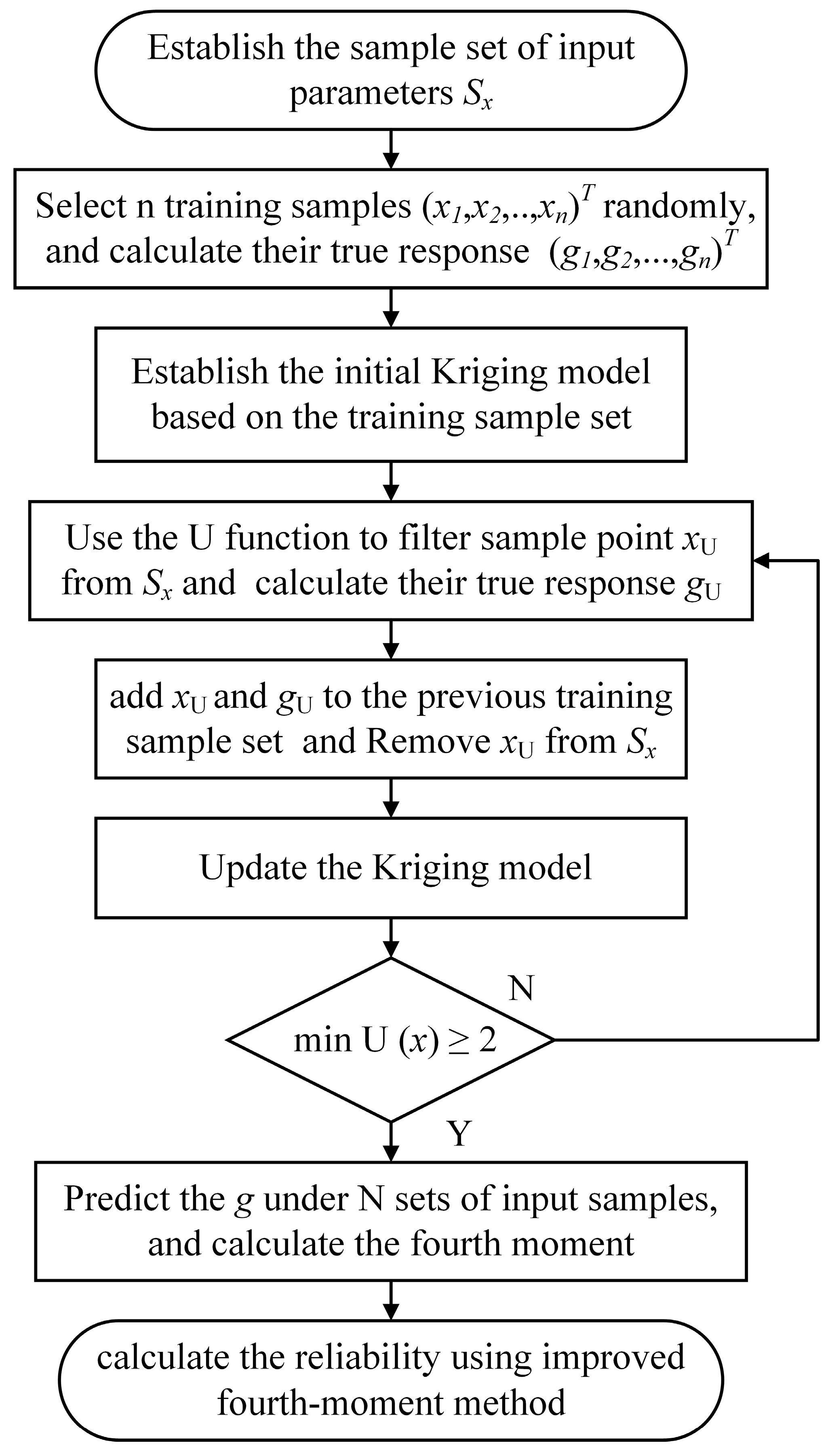
The convergence condition of the updating process is typically chosen as min U(x) ≥ 2, when the maximum probability of the model identification error is approximately 2.28%. The specific flow of the adaptive Kriging fourth-moment method (AK-FM) proposed in this paper is illustrated in Figure 1.

3. Results

The effectiveness and accuracy of the proposed AK-FM method can be verified by analyzing the reliability calculation results under the conditions of the explicit preset state function and implicit complex stress–strength state function for rolling bearings, respectively. Finally, an example of a smooth time-varying fatigue reliability analysis under the implicit state function of rolling bearings is used to verify the efficiency of the method.

3.1. Reliability Analysis with Explicit State Function

In order to verify the effectiveness of the method proposed in this paper, four types of explicit nonlinear state functions are set up by considering two-parameter input variables $\left(x,y\right)$ as follows:

• Exponential: $g_a\left(x,y\right)=e^x-y$;
• Power law: $g_b\left(x,y\right)=x^2-y$;
• Trigonometric: $g_c\left(x,y\right)=cosx-siny$;
• Segmented functional: $g_d\left(x,y\right)=\begin{array}{cc}x-siny& x\ge 0\\ -x-siny& x<0\end{array}$.

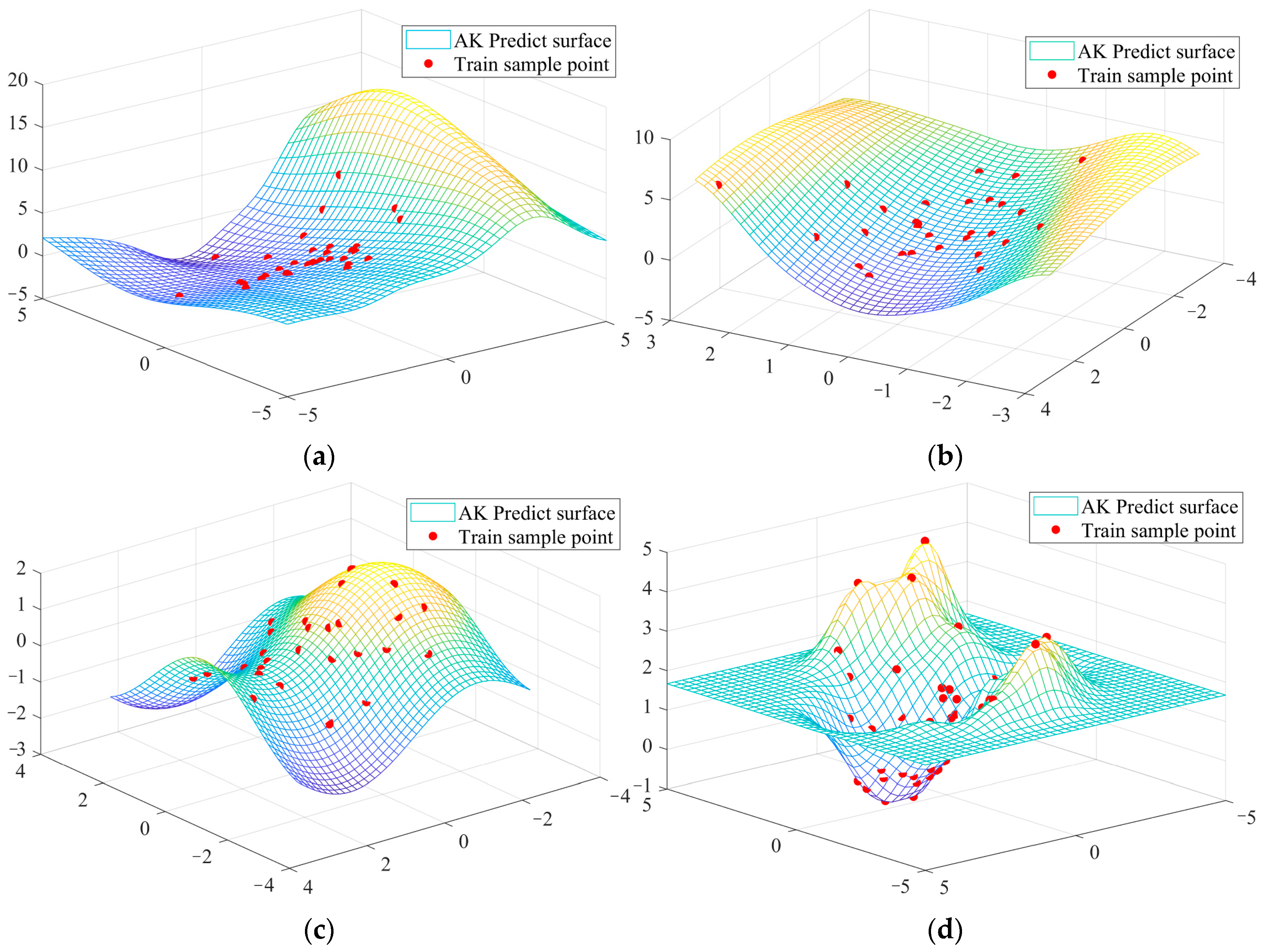
Based on the above four nonlinear state functions, using the method proposed in this paper, 1000 groups of $x,y~N\left(0,1\right)$ are selected to construct the input sample set, and the initial training set is selected to train the adaptive Kriging agent model by selecting the first 25 groups; the corresponding Kriging-predicted response surfaces and training points of the four types of state functions are shown in Figure 2, and it can be seen that the response surfaces of the various functions are well fitted. The response surfaces corresponding to the exponential, power, and trigonometric state functions are depicted in (a), (b), and (c), respectively. It is evident that these response surfaces exhibit a relatively smooth nature. Additionally, the response surface of the segmented state function, illustrated in (d), aligns well with the sample points despite the significant local variability of the surface.

The reliability results calculated using the AK-FM method proposed in this paper are compared with those calculated using the MCS method with a total number of samples of ${10}^6$, as shown in

Table 1. A comparison of reliability in the case of explicit state function.

State Function	Method	Total Sample Size	Initial Sample Size	Increased Sample Size	U Function Value	Reliability	Number of State Function Calls
Exponential	AK-FM	1000	25	7	2.3870	0.8144	32
	MCS	${10}^6$	\	\	\	0.8249	${10}^6$
Power law	AK-FM	1000	25	4	3.5760	0.7220	29
	MCS	${10}^6$	\	\	\	0.7193	${10}^6$
Trigonometric	AK-FM	1000	25	6	3.0884	0.7852	31
	MCS	${10}^6$	\	\	\	0.7681	${10}^6$
Segmented functional	AK-FM	1000	25	47	3.1502	0.8183	72
	MCS	${10}^6$	\	\	\	0.7901	${10}^6$

. Since the MCS method is calculated directly by corresponding to the explicit state function, it can be recognized as an exact solution. Most of the explicit state functions in the reliability analysis of mechanical products can be represented by the above four nonlinear functions, so the above results are sufficient to show the accuracy and validity of the proposed method applied to the explicit state function reliability analysis problem.

As can be seen from Table 1, on the one hand, the two methods do not have much error in the calculation results for four different types of state functions, but the proposed method requires a significantly smaller sample size than the MCS method. On the other hand, for the continuous state functions of exponential, power law, and trigonometric type, the number of updates of the Kriging model is smaller, and the model’s training speed is very fast; for the segmented state functions, the Kriging model needs more updates, which indicates that more samples are needed to achieve a certain prediction accuracy for the complex state functions, even though the number of calls of the state functions in this paper is still much less than that of the MCS method.

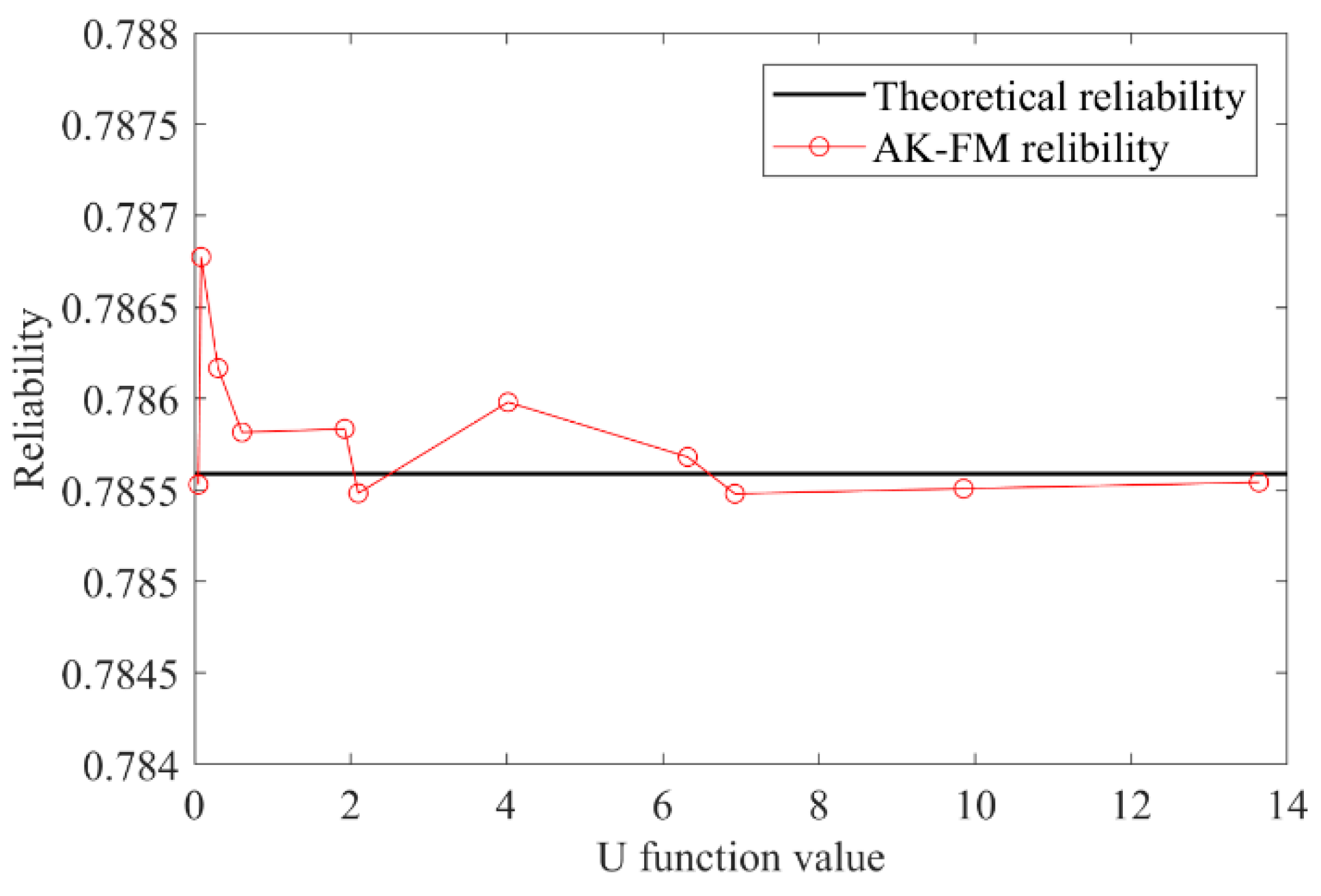
An intriguing question is whether the AK-FM proposed in this paper can obtain more accurate reliability results as the U function threshold increases. Therefore, taking the reliability calculation with the trigonometric state function as an example, different U constraint values are selected as the convergence judgment conditions and calculated using the method proposed in this paper; in order to ignore the inherent error between the MCS and the fourth-moment method, the calculated results of the fourth-moment method with a sample size of ${10}^6$ are used as the theoretical true value for this comparison, and the comparison results are shown in Figure 3.

A known conclusion is that the larger the U function, the better the Kriging model is fitted around the state function [34]. However, as can be seen in Figure 3, the error between the reliability results and the theoretical truth is not monotonically decreasing because an inaccurate Kriging model can also incorrectly produce reliability results when the value of the U function is less than a certain level (e.g., less than 2). When the critical value of the U function is set to a certain level (e.g., greater than 6) and the number of predicted samples is large enough, the reliability results will eventually converge to the theoretical true value.

In the case of the explicit nonlinear state function, the overall reliability calculation results obtained using the AK-FM method proposed in this paper are in good agreement with those obtained using the MCS method, and the number of calls to the state function is greatly reduced, although the cost of the explicit state function calls in this case is very low, and the difference between the two methods in terms of the total computation time is not obvious. However, when taking into account the high cost of the complex state function calls in actual engineering, the proposed method is able to significantly improve the efficiency of the reliability calculation.

3.2. Reliability Analysis of Implicit State Function for Rolling Bearing

Rolling bearing is a complex assembly composed of rollers, raceways, and cages whose working conditions and dimensional parameters affect the contact load between rollers and raceways, and thus, the performance of rolling bearings [40]. Existing mechanical modeling methods offer improved accuracy in calculating the contact load between the roller and raceway compared to previous methods, but they still fall short of the precision achieved by the finite element method. This study proposes establishing a finite element model based on input working conditions and size parameters to accurately calculate the contact load between the roller and raceway. The determination of the bearing qualification is based on whether the contact load exceeds a critical value, presenting a typical complex implicit equation of state problem. This paper takes the deep groove ball bearing 6016 as an example, and its working conditions are as follows: outer diameter, $D=125 \mathrm{m}\mathrm{m}$; inner diameter, $d=80 \mathrm{m}\mathrm{m}$; number of balls, $\mathrm{Z}=20$; rotating speed, $n=1000 \mathrm{r}/\mathrm{m}\mathrm{i}\mathrm{n}$; radial force, $F_r=500 \mathrm{N}$; material GCr15; elastic modulus, $E=208 \mathrm{G}\mathrm{P}\mathrm{a}$; Poisson’s ratio, $v=0.3$; and hardness, $HB=200$.

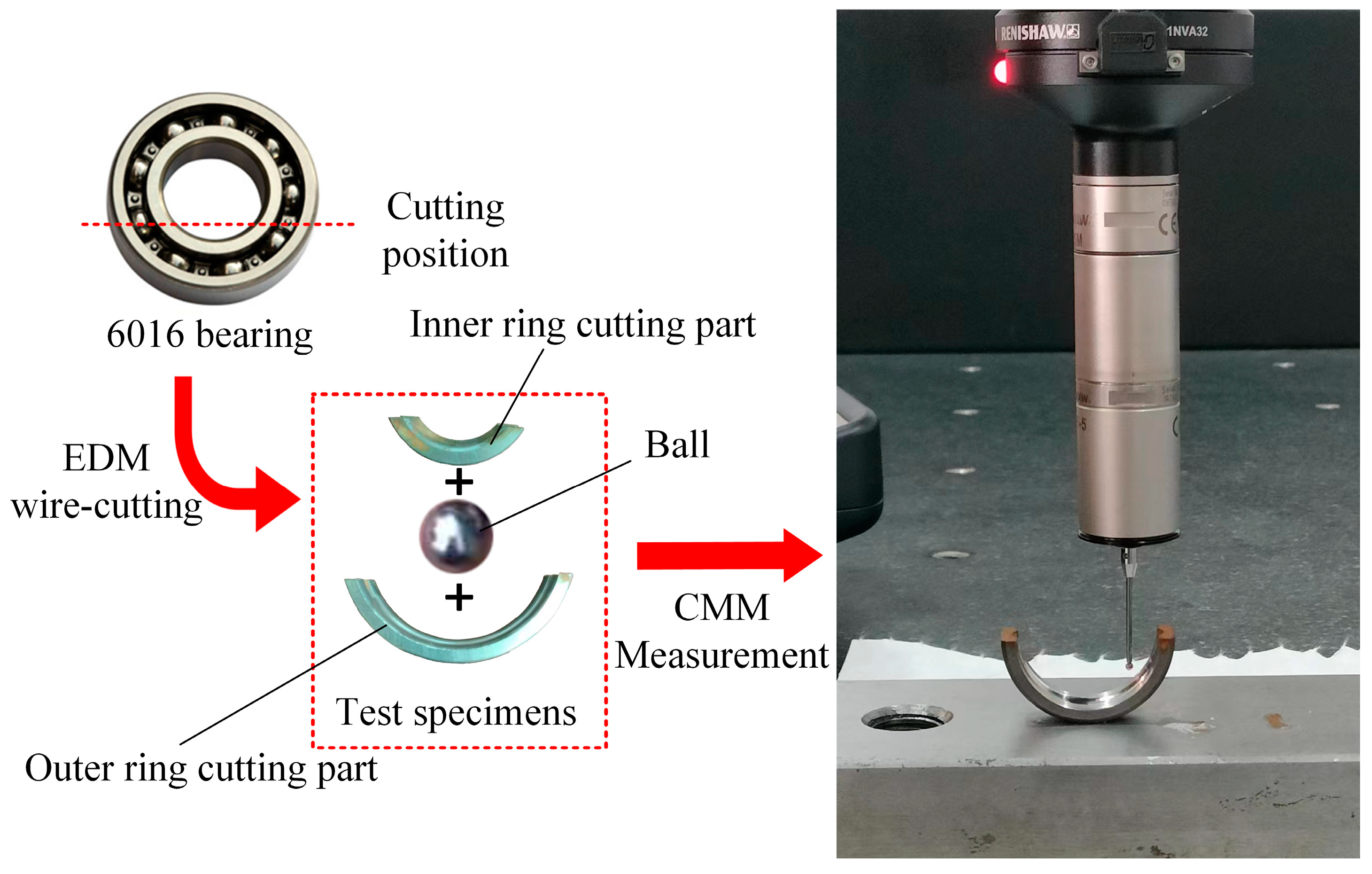
We seleted the design parameters and constructed the input parameter vector $\mathit{X}={\left[D_m,D_w,R_i,R_o\right]}^T$. Ten 6016 bearings with the same precision produced by the same manufacturer were selected and cut into 10 groups of specimens by EDM wire cutting, and the dimensional parameter data of the specimens were obtained by measuring with the CMM, as shown in Figure 4, respectively. According to the calculation results of these 10 groups of data, the moments of each size parameter in $\mathit{X}$ were obtained. The remaining parameters were obtained according to the method described in reference [41] and are shown in

Table 2. Random parameters of 6016 bearing input.

Bearing Parameters	Mean	Variance
Ball diameter $D_w$ (mm)	13.4940	4.0 × 10−6
Centre circle diameter $D_m$ (mm)	102.4874	2.5 × 10−5
Inner ring groove radius $R_i \left(\mathrm{m}\mathrm{m}\right)$	7.1010	1.0 × 10−6
Outer ring groove radius $R_o$ (mm)	6.9960	1.0 × 10−6

.

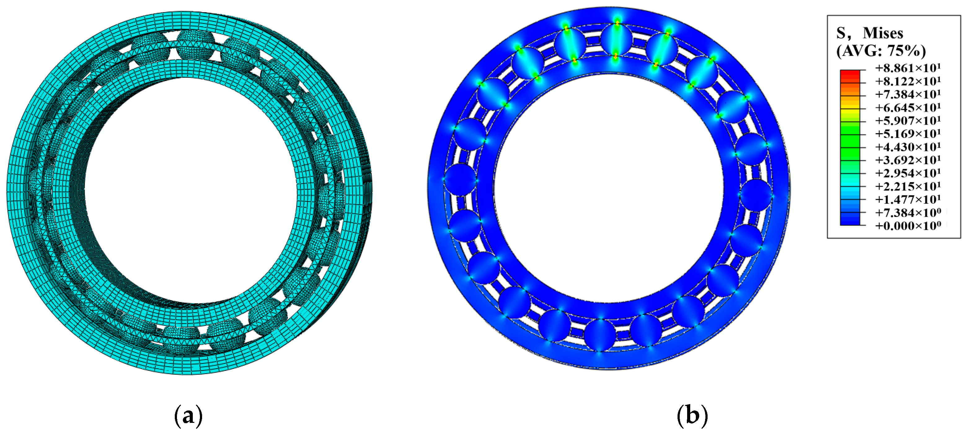
Based on the data presented in Table 2, a total of 100 sets of input parameter vector samples were randomly generated. From these, 20 sets were selected as the training sample set and analyzed using a finite element model for stress simulation. The interactions between the inner ring and the roller, as well as between the roller and the outer ring, were considered in this model, with all contact surfaces assumed to be smooth. All components were made of GCr15 material. The outer ring was constrained and completely fixed, while a radial concentrated force was applied to the inner surface of the inner ring coupled to the center point. The maximum contact stress ${\sigma }_{max}\left(\mathit{X}\right)$ under the current operating conditions was then determined, as shown in Figure 5. An initial Kriging model was established between the training sample set and ${\sigma }_{max}\left(\mathit{X}\right)$, which was subsequently updated and optimized using the proposed method.

Assuming the maximum threshold value of contact stress $\widehat{\sigma }$ based on material properties, the contact state function of rolling bearing 6016 can be defined as follows:

$$g_{6016}=\widehat{\sigma }-{\sigma }_{max}\left(\mathit{X}\right)$$

(24)

Obviously, when $g_{6016}\ge 0$, it is in a safe state, and when $g_{6016}<0$, it is in a failed state.

For the above 6016 bearing contact state function, the reliability results calculated using the method proposed in this paper are compared with the results obtained using the AK-MCS method, as shown in

Table 3. Comparison of contact reliability results for 6016 bearings.

Method	Initial Sample Size	Increased Sample Size	U Function Value	Number of State Function Calls	Number of State Function Predictions	Reliability
AK-FM	20	4	4.4659	24	1000	0.7087
AK-MCS	20	4	4.4659	24	${10}^6$	0.7086

.

As shown in Table 3, the two methods are based on exactly the same adaptive Kriging model under finite samples, and the difference in the reliability calculation results is very small, but the number of predictions of the state function of the proposed AK-FM method in this paper is much lower than that of the AK-MCS method, which is much more advantageous in terms of computational efficiency.

3.3. Reliability Analysis under Smooth Time-Varying State Function for Rolling Bearing

The efficiency advantage of the proposed AK-FM method over the AK-MCS method will be more pronounced when extended to the time-varying reliability problem, considering the cumulative cost of reliability computation at successive single time points.

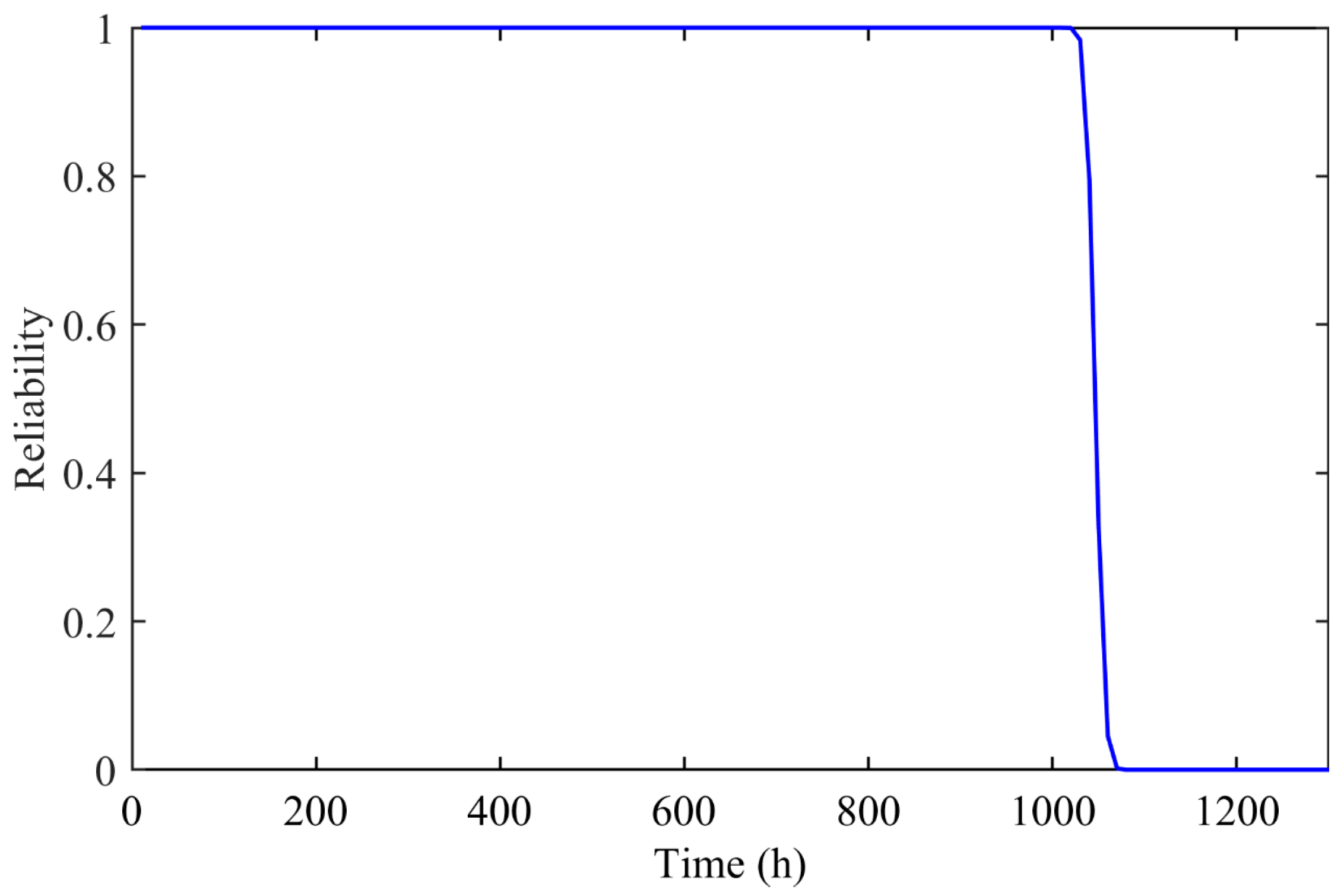
On the basis of the rolling bearing contact reliability calculation example, by considering the rolling bearing smooth time-varying fatigue accumulation damage [41], we constructed the 6016 bearing fatigue state function $g_{f6016}$ as follows:

$$g_{f6016}=1-\frac{∆D_{rb}\left(\mathit{X}\right)}{T}\times t$$

(25)

By using the method proposed in this paper to calculate the reliability and setting the time interval at $∆t=10 \mathrm{h}$, the curve of reliability over time can be obtained as shown in Figure 6.

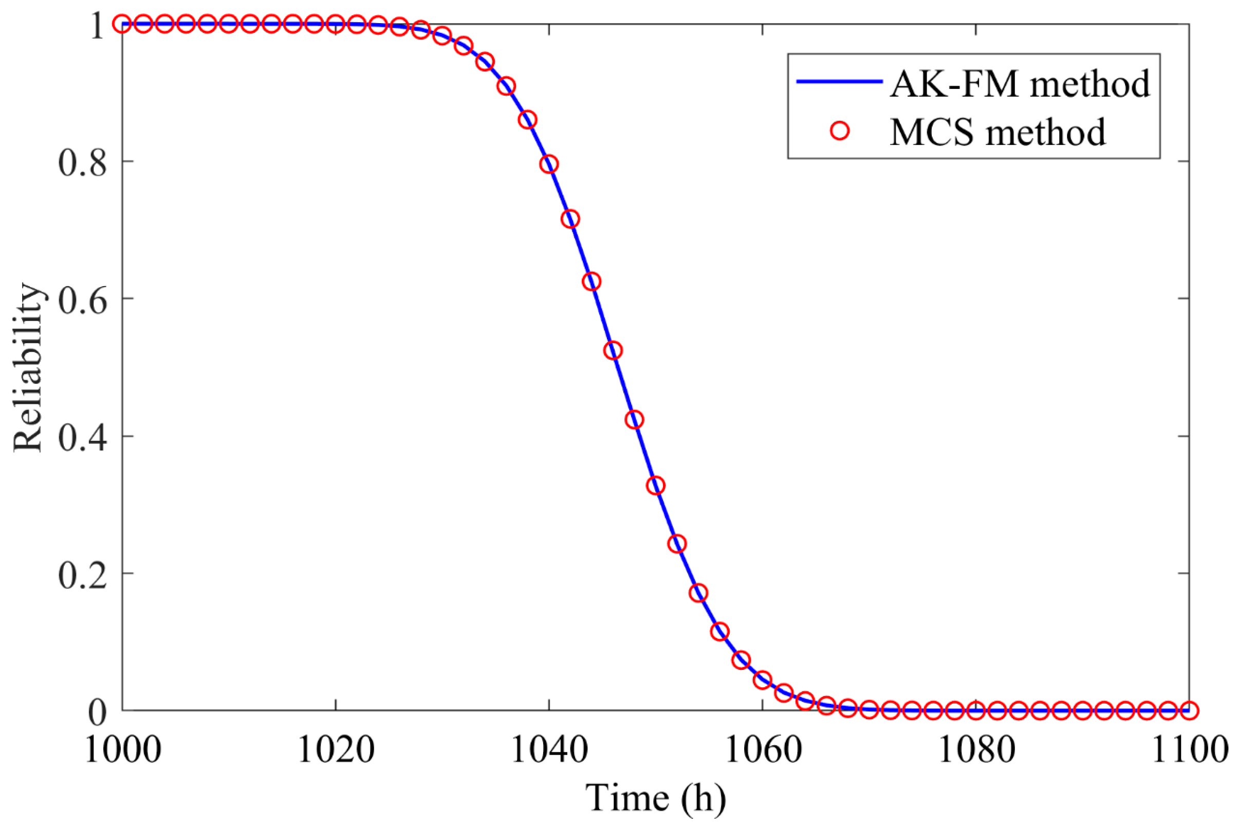
We selected the time period of 1000–1100 h, where the reliability curve changes more drastically, and the reliability curve over time calculated using the method proposed in this paper is compared with the reliability curve calculated using the AK-MCS method, as shown in Figure 7.

It can be seen that in the interval of 1000–1100 h, the results of the two methods are basically the same. The time points t = 1040 h, t = 1050 h, and t = 1060 h are further selected to compare the reliability results of the proposed method with the state function prediction of 1000 and 10,000 times and the AK-MCS reliability calculation with the state function prediction of ${10}^6$ times, as shown in

Table 4. Reliability comparison at different time points.

Time Point	Method	Initial Sample Size	Increased Sample Size	U Function Value	Number of State Function Predictions	Reliability
t = 1040 h	AK-FM	10	4	3.2139	1000	0.7862
	AK-FM	10	4	3.2139	10,000	0.7907
	AK-MCS	10	4	3.2139	${10}^6$	0.7955
t = 1050 h	AK-FM	10	4	4.3016	1000	0.3143
	AK-FM	10	4	4.3016	10,000	0.3269
	AK-MCS	10	4	4.3016	${10}^6$	0.3288
t = 1060 h	AK-FM	10	4	3.2908	1000	0.0416
	AK-FM	10	4	3.2908	10,000	0.0442
	AK-MCS	10	4	3.2908	${10}^6$	0.0448

.

From the results in Table 4, it can be seen that, on the one hand, the computational results of the method proposed in this paper have less error with the AK-MCS method at different time points, while the number of times the state function is predicted is smaller. On the other hand, it is obvious that the results of the proposed method for 10,000 state function predictions are more accurate relative to the proposed method for 1000 state function predictions, indicating that the accuracy of the proposed method increases with the increase in the number of state function predictions. It is demonstrated that the proposed AK-FM method can be used for reliability computation under a smooth time-varying state function, and that it can accurately and efficiently perform the reliability computation at a single time point with the appropriate number of state function prediction sets.

4. Discussion

In this paper, we propose an adaptive Kriging-based fourth-moment method (AK-FM) for an efficient reliability analysis under limited sample conditions. When the distribution of the random variable is difficult to determine due to limited available samples, we adopt the fourth-moment method to construct a fourth-order moment reliability index. To establish a surrogate model between the moments of the random variables and the moments of the complex state function, we employ the Kriging method and update the Kriging model based on the U function. We use the adaptive Kriging model to generate state function prediction samples, approximating the first four moments of the state function, and utilize the fourth-moment method for the reliability analysis. The main contribution of our method is that it overcomes the challenge of computing or incurring high costs for the moments of complex state functions, which is a limitation of existing fourth-moment methods. Additionally, our method inherits the efficiency advantage of the moment method over the simulation method compared to the existing AK-MCS method, and it can be applied in time-varying reliability analysis. Several numerical examples demonstrate that our proposed method achieves a comparable computational accuracy to the MCS method or the AK-MCS method, even with an inadequate sample size. Furthermore, it significantly improves the computational efficiency for a reliability analysis of engineering structures with complex state functions.

References

- Metropolis, N.; Ulam, S. The monte carlo method. J. Am. Stat. Assoc. 1949, 44, 335–341. [Google Scholar] [CrossRef] [PubMed]
- Kroese, D.P.; Brereton, T.; Taimre, T.; Botev, Z.I. Why the Monte Carlo method is so important today. Wiley Interdiscip. Rev. Comput. Stat. 2014, 6, 386–392. [Google Scholar] [CrossRef]
- Allaix, D.L.; Carbone, V.I. An improvement of the response surface method. Struct. Saf. 2011, 33, 165–172. [Google Scholar] [CrossRef]
- Zhang, D.; Han, X.; Jiang, C.; Liu, J.; Li, Q. Time-dependent reliability analysis through response surface method. J. Mech. Des. 2017, 139, 41404. [Google Scholar] [CrossRef]
- Der Kiureghian, A.; Ke, J. The stochastic finite element method in structural reliability. Probabilistic Eng. Mech. 1988, 3, 83–91. [Google Scholar] [CrossRef]
- Shao, Z.; Li, X.; Xiang, P. A new computational scheme for structural static stochastic analysis based on Karhunen–Loève expansion and modified perturbation stochastic finite element method. Comput. Mech. 2023, 71, 917–933. [Google Scholar] [CrossRef]
- Lee, K.; Cho, H.; Lee, I. Variable selection using Gaussian process regression-based metrics for high-dimensional model approximation with limited data. Struct. Multidiscip. Optim. 2019, 59, 1439–1454. [Google Scholar] [CrossRef]
- Moon, M.; Kim, H.; Lee, K.; Park, B.; Choi, K.K. Uncertainty quantification and statistical model validation for an offshore jacket structure panel given limited test data and simulation model. Struct. Multidiscip. Optim. 2020, 61, 2305–2318. [Google Scholar] [CrossRef]
- Efron, B.; Tibshirani, R.J. An Introduction to the Bootstrap; CRC Press: Boca Raton, FL, USA, 1994; ISBN 0412042312. [Google Scholar]
- Amalnerkar, E.; Lee, T.H.; Lim, W. Reliability analysis using bootstrap information criterion for small sample size response functions. Struct. Multidiscip. Optim. 2020, 62, 2901–2913. [Google Scholar] [CrossRef]
- Al Luhayb, A.S.M.; Coolen, F.P.; Coolen-Maturi, T. Smoothed bootstrap for right-censored data. Commun. Stat.-Theory Methods 2023, 1–25. [Google Scholar] [CrossRef]
- De Campos, L.M.; Huete, J.F.; Moral, S. Probability intervals: A tool for uncertain reasoning. Int. J. Uncertain. Fuzziness Knowl.-Based Syst. 1994, 2, 167–196. [Google Scholar] [CrossRef]
- Ferson, S.; Kreinovick, V.; Ginzburg, L.; Sentz, F. Constructing Probability Boxes and Dempster-Shafer Structures; Sandia National Laboratories (SNL-NM): Albuquerque, NM, USA, 2003. [Google Scholar]
- Zhang, H.; Dai, H.; Beer, M.; Wang, W. Structural reliability analysis on the basis of small samples: An interval quasi-Monte Carlo method. Mech. Syst. Signal Proc. 2013, 37, 137–151. [Google Scholar] [CrossRef]
- Zhao, Y.; Ono, T. Moment methods for structural reliability. Struct. Saf. 2001, 23, 47–75. [Google Scholar] [CrossRef]
- Hohenbichler, M.; Rackwitz, R. First-order concepts in system reliability. Struct. Saf. 1982, 1, 177–188. [Google Scholar] [CrossRef]
- Hasofer, A.M.; Lind, N.C. Exact and invariant second-moment code format. J. Eng. Mech. Div. 1974, 100, 111–121. [Google Scholar] [CrossRef]
- Zhang, T. An improved high-moment method for reliability analysis. Struct. Multidiscip. Optim. 2017, 56, 1225–1232. [Google Scholar] [CrossRef]
- Tichý, M. First-order third-moment reliability method. Struct. Saf. 1994, 16, 189–200. [Google Scholar] [CrossRef]
- Zhao, Y.; Lu, Z.; Ono, T. A simple third-moment method for structural reliability. J. Asian Archit. Build. Eng. 2006, 5, 129–136. [Google Scholar] [CrossRef]
- Zhao, Y.; Lu, Z. Fourth-moment standardization for structural reliability assessment. J. Struct. Eng. 2007, 133, 916–924. [Google Scholar] [CrossRef]
- Zhang, T. Matrix description of differential relations of moment functions in structural reliability sensitivity analysis. Appl. Math. Mech. 2017, 38, 57–72. [Google Scholar] [CrossRef]
- Kudela, J.; Matousek, R. Recent advances and applications of surrogate models for finite element method computations: A review. Soft Comput. 2022, 26, 13709–13733. [Google Scholar] [CrossRef]
- Emad, W.; Mohammed, A.S.; Kurda, R.; Ghafor, K.; Cavaleri, L.; Qaidi, S.M.; Hassan, A.; Asteris, P.G. Prediction of concrete materials compressive strength using surrogate models. Structures 2022, 46, 1243–1267. [Google Scholar] [CrossRef]
- Ma, Y.; Jin, X.; Wu, X.; Xu, C.; Li, H.; Zhao, Z. Reliability-based design optimization using adaptive Kriging-A single-loop strategy and a double-loop one. Reliab. Eng. Syst. Saf. 2023, 237, 109386. [Google Scholar] [CrossRef]
- Song, Z.; Liu, Z.; Zhang, H.; Zhu, P. An improved sufficient dimension reduction-based Kriging modeling method for high-dimensional evaluation-expensive problems. Comput. Meth. Appl. Mech. Eng. 2024, 418, 116544. [Google Scholar] [CrossRef]
- Nan, H.; Liang, H.; Di, H.; Li, H. A gradient-assisted learning strategy of Kriging model for robust design optimization. Reliab. Eng. Syst. Saf. 2024, 244, 109944. [Google Scholar] [CrossRef]
- Tripathy, R.K.; Bilionis, I. Deep UQ: Learning deep neural network surrogate models for high dimensional uncertainty quantification. J. Comput. Phys. 2018, 375, 565–588. [Google Scholar] [CrossRef]
- White, D.A.; Arrighi, W.J.; Kudo, J.; Watts, S.E. Multiscale topology optimization using neural network surrogate models. Comput. Meth. Appl. Mech. Eng. 2019, 346, 1118–1135. [Google Scholar] [CrossRef]
- Novák, L.; Sharma, H.; Shields, M.D. Physics-informed polynomial chaos expansions. J. Comput. Phys. 2024, 506, 112926. [Google Scholar] [CrossRef]
- Modak, A.; Chakraborty, S. An enhanced learning function for bootstrap polynomial chaos expansion-based enhanced active learning algorithm for reliability analysis of structure. Struct. Saf. 2024, 109, 102467. [Google Scholar] [CrossRef]
- Pan, Y.; Qin, J.; Hou, Y.; Chen, J. Two-stage support vector machine-enabled deep excavation settlement prediction considering class imbalance and multi-source uncertainties. Reliab. Eng. Syst. Saf. 2024, 241, 109578. [Google Scholar] [CrossRef]
- Hu, Z.; Tang, C.; Liang, Y.; Chang, S.; Ni, X.; Xiao, S.; Meng, X.; He, B.; Liu, W. Feature Detection Based on Imaging and Genetic Data Using Multi-Kernel Support Vector Machine–Apriori Model. Mathematics 2024, 12, 684. [Google Scholar] [CrossRef]
- Echard, B.; Gayton, N.; Lemaire, M. AK-MCS: An active learning reliability method combining Kriging and Monte Carlo simulation. Struct. Saf. 2011, 33, 145–154. [Google Scholar] [CrossRef]
- Zhao, D.; Ma, M.; You, X. A Kriging-based adaptive parallel sampling approach with threshold value. Struct. Multidiscip. Optim. 2022, 65, 225. [Google Scholar] [CrossRef]
- Wang, T.; Chen, Z.; Li, G.; He, J.; Liu, C.; Du, X. A novel method for high-dimensional reliability analysis based on activity score and adaptive Kriging. Reliab. Eng. Syst. Saf. 2024, 241, 109643. [Google Scholar] [CrossRef]
- Liu, Z.; Lu, Z.; Ling, C.; Feng, K.; Hu, Y. An improved AK-MCS for reliability analysis by an efficient and simple reduction strategy of candidate sample pool. Structures 2022, 35, 373–387. [Google Scholar] [CrossRef]
- Afshari, S.S.; Enayatollahi, F.; Xu, X.; Liang, X. Machine learning-based methods in structural reliability analysis: A review. Reliab. Eng. Syst. Saf. 2022, 219, 108223. [Google Scholar] [CrossRef]
- Mai, H.T.; Lee, J.; Kang, J.; Nguyen-Xuan, H.; Lee, J. An Improved Blind Kriging Surrogate Model for Design Optimization Problems. Mathematics 2022, 10, 2906. [Google Scholar] [CrossRef]
- Shi, P.; Wu, S.; Xu, X.; Zhang, B.; Liang, P.; Qiao, Z. TSN: A novel intelligent fault diagnosis method for bearing with small samples under variable working conditions. Reliab. Eng. Syst. Saf. 2023, 240, 109575. [Google Scholar] [CrossRef]
- E, S.; Wang, Y.; Xie, B.; Lu, F. A Reliability-Based Robust Design Optimization Method for Rolling Bearing Fatigue under Cyclic Load Spectrum. Mathematics 2023, 11, 2843. [Google Scholar] [CrossRef]
Figure 1.
Process of AK-FM method.
Figure 2.
Predicted response surfaces and actual sample points. (a) Exponential. (b) Power law. (c) Trigonometric. (d) Segmented functional.
Figure 3.
Reliability for different U function thresholds.
Figure 4.
CMM measurement of 6016 bearing specimen.
Figure 5.
FEM simulation of 6016 bearing; (a) 6016 FEM meshing model and (b) 6016 FEM simulation results.
Figure 6.
Smooth time-varying fatigue reliability curve of 6016 bearing.
Figure 7.
Comparison of smooth time-varying fatigue reliability curves of 6016.