A Multi-Stage Constraint-Handling Multi-Objective Optimization Method for Resilient Microgrid Energy Management

Abstract

In recent years, renewable energy has seen widespread application. However, due to its intermittent nature, there is a need to develop energy management systems for its scheduling and control. This paper introduces a multi-stage constraint-handling multi-objective optimization method tailored for resilient microgrid energy management. The microgrid encompasses diesel generators, energy storage systems, renewable energy sources, and various load types. The intelligent management of generators, batteries, switchable loads, and controllable loads ensures a reliable power supply for the critical loads. Beyond operational costs, our model also considers grid dependency as a key objective, making it particularly suited for energy management in extreme environments such as islands, border regions, and military bases. Managing complex controls of generators, batteries, switchable loads, and controllable loads presents challenging constraints that the management strategy must meet. To tackle this challenge, we propose an multi-objective optimization algorithm with multi-stage constraint-handling strategy to handle the high-dimensional complex constraints of the resilient energy management problem. Our proposed approach demonstrates superior performance compared to nine leading constrained multi-objective optimization algorithms across various test scenarios. Furthermore, the benefits of our method become increasingly evident as the complexity of the problem increases. Compared to the classical NSGA-II, the proposed NSGA-II-MC method achieved a 49.7% improvement in the Hypervolume metric on large-scale problems.

1. Introduction

The scarcity of fossil fuels and growing concerns about global warming have led to the emergence of renewable energy sources. Microgrids, which coordinate various renewable energy resources, distributed generators, energy storage systems, and electrical loads alongside the conventional power grid, are a promising technique to mitigate the depletion of fossil fuels and to reduce the associated carbon footprint. However, the high penetration of renewable energy resources, such as solar power and wind power, imposes new challenges in the operation of microgrids because of their intermittent nature. To address the uncertainties posed by these intermittent power sources, energy management systems have been increasingly developed to increase the reliability of microgrids and to yield better performance. Energy management is defined as an approach to optimize the utilization of controllable devices in a microgrid to minimize its operation cost, emissions, and other objectives. This work focuses on the resilient energy management of microgrids, where, in addition to generators and storage units, various switchable and controllable loads can be strategically scheduled to meet the electricity demand of critical loads under extreme environmental conditions, such as islands, border regions, and military bases. In these scenarios, access to the main power grid may be uncertain or prohibitively expensive. Introducing control over various switchable and controllable loads makes the optimization problem of energy management more difficult to solve, as it exhibits the typical characteristics of being large-scale, multi-objective, and multi-constraint. Therefore, developing effective solution algorithms is especially necessary.

In recent years, diverse methods including mathematical programming-based optimization approaches and meta-heuristic algorithms have been proposed [1] for energy management. Zhang et al. [2] tackled the energy management problem by employing particle swarm optimization, taking into account the integration of photovoltaic systems and batteries while considering energy tariff rates. Liu et al. [3] delved into a stochastic optimization model, focusing on curtailing net generation costs considering real-time market prices. Badawy and Sozer [4] introduced a supervisory energy management method that amalgamates fuzzy logic controllers with sliding mode control, ensuring a stable power supply and uninterrupted energy delivery. Tanvir and Merabet [5] introduced an energy management approach that seamlessly integrates batteries with wind energy systems, placing significant importance on monitoring battery State of Charge (SoC) for effective battery charging and discharging. Roy et al. [6] proposed a novel approach that leverages artificial neural networks in conjunction with hybrid whale optimization to minimize generation costs while forecasting renewable energy availability. Li et al. [7] developed an encompassing energy management system that optimizes the simultaneous operation of thermal and battery systems, resulting in improved frequency and voltage stability within microgrid networks. Pannala et al. [8] engaged in a comprehensive exploration of voltage control and energy management strategies, employing an exhaustive approach across both isolated and grid-connected microgrid systems. This approach addresses critical challenges, including generation failures, low power generation, and battery constraints. Oliveira-Assis et al. [9] proposed an optimized energy management approach that harnesses biogeography-based modeling to minimize hydrogen fuel consumption within charging-station-based microgrid systems. Zhao et al. [10] devised an optimal scheduling strategy employing model predictive control to bolster system resilience in the face of renewable energy variability. This strategy finds practical application in multi-microgrid scenarios, especially under dynamic trading conditions. Merabet et al. [11] presented an energy management framework with a dual focus on reducing generation costs and optimizing battery usage. This solution also integrates load-shifting mechanisms and adapts to varying grid tariffs. Moreover, various approaches have been proposed to address the critical presence of uncertain data in energy management optimization problems. Nammouchi et al. [12] proposed to combine Machine Learning and Robust Optimization for optimally scheduling energy generation, consumption, and buy/sell actions in a microgrid, taking into account the uncertainty of photovoltaic power generation and user consumption. Chen et al. [13] adopted chance-constrained programming for modeling and solving an uncertain multi-objective microgrid scheduling problem, addressing the uncertainty of renewable energy generation. Rui et al. [14] combined Mixed Integer Programming and Stackelberg games for defining an optimal energy scheduling in a microgrid context. Vidan et al. [15] proposed a computationally efficient Robust Optimization method for tackling energy price data uncertainty while optimally managing production and battery storage actions. However, it should be noted that existing single-objective optimization methods for energy management rarely consider the control of controllable loads, and most of them only utilize existing optimization methods without designing proprietary methods for the complex and high-dimensional constraints present in energy management problems. Consequently, the convergence capability of these methods may be limited.

Various objectives such as cost, emissions, and battery lifespan should be considered when supplying the load. Consequently, the necessity of multi-objective optimization algorithms becomes apparent. In this context, Li and Xia [16] introduced the Non-dominated Sorting Genetic Algorithm II (NSGA-II) method as an effective means to address multiple objectives within microgrid management, with a particular emphasis on reducing operating costs and mitigating air pollutants. Incorporating grid power consumption cost and battery degradation cost, Preetha Roselyn et al. [17] developed a multi-objective genetic algorithm similar to NSGA-II to optimize the energy management strategy in microgrids. Murty and Kumar [18] presented a multi-objective optimization framework to obtain the optimal energy dispatch strategy for grid-connected and standalone microgrids integrated with photovoltaic cells, wind turbines, fuel cells, micro turbines, diesel generators, and battery energy storage system. This method aims to minimize the costs of main grid energy, fuel costs, emissions, and other objectives. A multi-objective grey wolf method is proposed in [19] to obtain the Pareto front considering the opposing objectives of energy system cost and battery lifespan. In this work, sizing optimization and energy management strategy are both analyzed. De Kamal and Mandal [20] proposed a multi-objective modified personal best particle swarm optimization method for multi-microgrids energy management. This work aims to find the Pareto front of minimizing both operation costs and power losses. Li et al. [21] addressed a wide spectrum of objectives, including power quality, security, and financial considerations, in their quest to optimize energy scheduling within microgrids. Rajagopalan et al. [22] considered a variant of nature-inspired metaheuristics for multi-objective power generation scheduling.

Other multi-objective methods [23,24,25] have also been proposed for energy management of microgrids considering various objectives and microgrid properties. However, most existing works directly used off-the-shelf multi-objective algorithms, which might perform poorly on energy management problems with hard constraints. Given the substantial number of controllable loads, each with specific on/off timings and power demand constraints, the optimization problem becomes challenging to converge. In this context, we designate a multi-stage constraint-handling multi-objective optimization method for resilient microgrid energy management, and compare it with state-of-the-art multi-objective optimization algorithms. The contributions of this work are as follows:

• A resilient microgrid energy management model that incorporates the scheduling of diesel generators, energy storage systems, switchable loads, and controllable loads;
• A multi-stage constraint-handling multi-objective optimization algorithm that can effectively tackle the complex constraints of the resilient microgrid energy management problem;
• Superior performance compared to nine state-of-the-art constrained multi-objective optimization algorithms.

The rest of this paper is structured as follows: Section 2 outlines the model for the resilient microgrid energy management problem. The proposed constrained multi-objective optimization algorithm is elaborated upon in Section 3. Section 4 presents the experimental results, and Section 5 offers the conclusion.

2. System Model

This work focuses on the resilient energy management problem, primarily addressing extreme environments such as islands, border regions, and military bases. Our goal is to reduce the dependence on the main power grid in these areas. Given the limited energy resources and the necessity to meet critical loads due to specific scenarios, not only are storage and generators managed but loads are also controllable in this approach. This approach ensures that essential services and operations remain uninterrupted, even under challenging conditions. Therefore, given a microgrid composed of diesel generators, renewable energy sources, energy storage systems (such as batteries), and various loads, we aim to optimize the operation schedule for generators, energy storage, and controllable loads. This scheduling will take into account the operational constraints of each component to minimize both the operational costs and reliance on the main electricity grid.

Table 1. Mathematical Notations.

Symbol	Explanation
$P_{\mathrm{bess}}^{min}$	Minimum power output of the energy storage system
$P_{\mathrm{bess}}^{max}$	Maximum power output of the energy storage system
$P_{\mathrm{bess}}\left(k\right)$	Power output of the energy storage system at time k
$E_{\mathrm{bess}}^{min}$	Minimum energy capacity of the energy storage system
$E_{\mathrm{bess}}^{max}$	Maximum energy capacity of the energy storage system
$E_{\mathrm{bess}}\left(k\right)$	Energy capacity of the energy storage system at time k
${\eta }_{\mathrm{bess}}$	Charge/discharge efficiency of the energy storage system
${\epsilon }_{\mathrm{bess}}$	Self-discharge rate of the energy storage system
$\Delta P_{DG}$	Maximum ramping power of the diesel generator
$P_{DG}\left(k\right)$	Power output of the diesel generator at time k
$P_{DG}^{min}$	Minimum power output of the diesel generator
$P_{DG}^{max}$	Maximum power output of the diesel generator
$t_{on}\left(k\right)$	Continuous running time of the generator at time k
$t_{off}\left(k\right)$	Continuous off time of the generator at time k
$T^{on}$	Minimum continuous running time required for the generator
$T^{off}$	Minimum continuous off time required for the generator
${\beta }_{cur}^{min}$	Minimum proportion of switchable loads
${\beta }_{cur}^{max}$	Maximum proportion of switchable loads
${\beta }_{cur}\left(k\right)$	Proportion of switchable loads at time k
$T_{\mathrm{start},i}$	Earliest start time for the i-th controllable load
$T_{\mathrm{finish},i}$	Latest stop time for the i-th controllable load
$T_{sch,i}$	Total operating time requirement for the i-th controllable load
$E_{sch,i}$	Total energy demand for the i-th controllable load
${\delta }_{sch,i}\left(k\right)$	Operating state of the i-th controllable load at time k
$P_{sch,i}^{min}$	Minimum power output for the i-th controllable load
$P_{sch,i}^{max}$	Maximum power output for the i-th controllable load
$C_1$	Operational costs of the system
$C_{DG}\left(k\right)$	Operating costs of the diesel generator at time k
$C_{BESS}\left(k\right)$	Operating costs of the energy storage system at time k
$C_{cur}\left(k\right)$	Penalty for load shedding at time k
$C_{grid}\left(k\right)$	Cost of buying and selling electricity at time k
$C_{fuel}\left(k\right)$	Fuel cost for the diesel generator at time k
$O{M}_{DG}$	Maintenance cost per unit time of generator operation
${\chi }_{DG}^{up}\left(k\right)$	Fixed costs for each startup of the diesel generator
${\chi }_{DG}^{down}\left(k\right)$	Fixed costs for each shutdown of the diesel generator
$a,b$	Constant coefficients of fuel cost for the diesel generator
$O{M}_{BESS}$	Maintenance cost per unit time for the energy storage system
$c_{BESS}^{switch}$	Cost associated with charging and discharging losses
${\alpha }_{cur,i}\left(k\right)$	Penalty coefficient for the i-th load shedding
${\beta }_{cur,i}\left(k\right)$	Power of the shed load for the i-th controllable load
${\eta }_{grid}\left(k\right)$	Electricity price for buying ($c_{grid}^{bur}\left(k\right)$) or selling ($c_{grid}^{sel}\left(k\right)$)
$C_2$	Optimization objective to minimize dependence on the main grid
${\lambda }_{grid}$	Power purchased from the main grid

gives the mathematical notation used in the model.

2.1. System Description

The microgrid case studied in this paper consists of a diesel generator, a wind turbine generator, a photovoltaic generator, an energy storage system, and various types of loads. The loads include critical loads, switchable loads, and controllable loads. Among them, the electrical demands of critical loads must be met. Depending on the actual situation, the electrical demands of switchable loads can be curtailed. As for controllable loads, under the conditions of meeting their total electrical demands and time constraints, their on/off times and power can be adjusted. The decision variables for energy management in this microgrid system are shown in

Table 2. Decision variables for energy management problem.

Decision Variables	Descriptions	Type
${\delta }_{DG}\left(k\right)$	on/off status of the diesel generator at time k	binary
$P_{DG}\left(k\right)$	output power of the diesel generator at time k (kW)	continuous
${\delta }_{\mathrm{bess}}\left(k\right)$	status of the BESS at time k	binary
$P_{\mathrm{bess}}\left(k\right)$	charging/discharging power of the BESS at time k (kW)	continuous
$T_{sch}^{on,i}$	start time of the $i\mathrm{th}$ controllable load	integer
$T_{sch}^{off,i}$	shutdown time of the $i\mathrm{th}$ controllable load	integer
$P_{sch,i}\left(k\right)$	power consumption of the $i\mathrm{th}$ controllable load at time k (kW)	continuous
${\beta }_{cur}\left(k\right)$	proportion of flexible load curtailment at time k (%)	continuous

, and by controlling the operation of the generation equipment, energy storage system, and smart loads, the system operation can be optimized.

For the decision variables representing the operational status of generators and controllable loads, 1 represents “on” and 0 represents “off”. As for the status of the energy storage system ${\delta }_{sch,i}\left(k\right)$, 1 represents “discharge”, $-1$ represents “charge”, and 0 represents “off”.

2.2. Model Constraints

2.2.1. Energy Storage System Constraints

Consider the following constraints for the energy storage system:

$$P_{\mathrm{bess}}^{min}\le P_{\mathrm{bess}}\left(k\right)\le P_{\mathrm{bess}}^{max}$$

(1)

$$E_{\mathrm{bess}}^{min}\le E_{\mathrm{bess}}\left(k\right)\le E_{\mathrm{bess}}^{max}$$

(2)

That is, it is necessary to satisfy the maximum charging and discharging power constraints of the energy storage system, and the battery capacity of the energy storage system must not exceed the maximum and minimum capacity values. The capacity of the energy storage system is calculated as follows:

$$\begin{array}{c}{E}_{\mathrm{bess}}(k+1)=E_{\mathrm{bess}}\left(k\right)+{\eta }_{\mathrm{bess}}{P}_{\mathrm{bess}}\left(k\right)\Delta t-{\epsilon }_{\mathrm{bess}}\Delta t\\ {\eta }_{\mathrm{bess}}=\left\{\begin{array}{cc}{\eta }_{\mathrm{bess}}^c,\hfill & P_{\mathrm{bess}}\left(k\right)>0\hfill \\ {\eta }_{\mathrm{bess}}^d,\hfill & P_{\mathrm{bess}}\left(k\right)\le 0\hfill \end{array}\right.\end{array}$$

(3)

where ${\eta }_{\mathrm{bess}}$ represents the charge/discharge efficiency, and ${\epsilon }_{\mathrm{bess}}$ represents the self-discharge rate of the battery.

2.2.2. Diesel Generator Constraints

For the diesel generator, we first need to consider its ramping power constraint:

$$-\Delta P_{DG}\le P_{DG}\left(k\right)-P_{DG}(k-1)\le \Delta P_{DG}$$

(4)

This means that the change in the generator’s power output between adjacent time periods cannot exceed $\Delta P_{DG}$. Additionally, the generator’s power output must not go beyond its maximum or minimum power limits:

$$P_{DG}^{\min }\le P_{DG}\left(k\right)\le P_{DG}^{\max }$$

(5)

Furthermore, we need to consider the minimum on/off duration constraints for the generator:

$$t_{on}\left(k\right)\ge T^{on}$$

(6)

$$t_{off}\left(k\right)\ge T^{off}$$

(7)

Here, $t_{on}\left(k\right)$ represents the current continuous running time of the generator, and $t_{off}\left(k\right)$ represents the current continuous off time of the generator. This means that the generator needs to run continuously for $T^{on}$ time periods before it can be turned off and must remain off for $T^{off}$ time periods before it can be turned on.

2.2.3. Load Constraints

The paper considers three types of typical loads: (1) critical loads; (2) switchable loads; and (3) controllable loads. Critical loads are associated with various critical tasks whose electricity demands must be met. Switchable loads are non-critical loads whose power can be adjusted based on the actual situation, such as ventilation equipment, air conditioning, etc. The proportion of switchable loads must satisfy the following constraint:

$${\beta }_{cur}^{min}\le {\beta }_{cur}\left(k\right)\le {\beta }_{cur}^{max}$$

(8)

Compared to critical loads, controllable loads have more flexible energy requirements and only need to meet their power supply needs within a predefined time range. The energy management system can schedule their power consumption during various time periods. Examples of controllable loads include production tasks in industrial microgrids, various devices awaiting charging, and electric vehicles awaiting charging. The paper considers various controllable loads, and for each controllable load, the following constraints must be satisfied.

The device must operate within the time range from $T_{\mathrm{start},i}$ to $T_{\mathrm{finish},i}$, where $T_{\mathrm{start},i}$ and $T_{\mathrm{finish},i}$ represent the earliest start time and the latest stop time for the i-th controllable load. Additionally, it is necessary to meet the total operating time requirement $T_{sch,i}$ and the total energy demand $E_{sch,i}$ for each controllable load:

$$\sum _{k=T_{\mathrm{start},i}}^{T_{\mathrm{finish},i}}{\delta }_{sch,i}\left(k\right)=T_{sch,i}$$

(9)

$$\sum _{k=T_{\mathrm{start},i}}^{T_{\mathrm{finish},i}}{P}_{sch,i}\left(k\right)\Delta t=E_{sch,i}$$

(10)

For each operating time period, the device’s operating power must satisfy the power upper and lower bounds:

$${\delta }_{sch,i}\left(k\right)P_{sch,i}^{min}\le P_{sch,i}\left(k\right)\le {\delta }_{sch,i}\left(k\right)P_{sch,i}^{max}$$

(11)

Furthermore, to prevent frequent start–stop cycles that may damage the device, once the device is turned on, it cannot be stopped during its operation. This constraint is satisfied by:

$$\sum _{\tau =k}^{k+T_{sch,i}-1}{\delta }_{sch,i}\left(\tau \right)\ge T_{sch,i}\left({\delta }_{sch,i}\left(k\right)-{\delta }_{sch,i}(k-1)\right)k=T_{start,i},\cdots ,T_{finish,i}-T_{sch,i}+1$$

(12)

2.2.4. Power Balance Constraints

Diesel generators, wind power, and photovoltaic power are the energy supply nodes, while critical loads, switchable loads, and controllable loads are the energy demand nodes. Energy storage systems and the main grid adjust their power flow to satisfy the following power balance constraints:

$$\begin{array}{cc}\hfill \sum _{i=1}^{N_{\mathrm{sch}}}{P}_{sch,i}\left(k\right)+& {\tilde{P}}_{\mathrm{cur}}\left(k\right)\left(1-{\beta }_{cur}\left(k\right)\right)+{\tilde{P}}_{cri}\left(k\right)\hfill \\ \hfill & ={\tilde{P}}_{\mathrm{solar}}\left(k\right)+{\tilde{P}}_{\mathrm{wind}}\left(k\right)+P_{DG}\left(k\right)+P_{\mathrm{grid}}\left(k\right)+P_{bess}\left(k\right)\hfill \end{array}$$

(13)

where the values of $P_{\mathrm{grid}}\left(k\right)$ and $P_{bess}\left(k\right)$ greater than 0 indicate that the main grid and energy storage system are supplying power to the microgrid.

2.3. Optimization Objectives

The objectives of the energy management for the resilient microgrid studied in this paper are to reduce the operational costs of the system and its dependence on the main grid. Based on the generation from renewable sources such as wind and photovoltaics, load usage, and electricity price information, the system aims to reduce costs by charging during low electricity price periods and discharging during high electricity price periods using the energy storage system. Through coordinated control of generation equipment, energy storage, and loads, the system also aims to decrease its reliance on the main grid. This approach has several benefits, including mitigating the impact of renewable energy fluctuations on the main grid, increasing the utilization of renewable energy, and enhancing the reliability of the microgrid system. It is suitable for energy management in extreme environments like islands, border regions, and military bases.

Therefore, the optimization objective of the microgrid consists of two parts: minimizing the operational costs of the system and minimizing the energy exchange between the microgrid and the main grid. The calculation of operational costs is as follows:

$$C_1=min\sum _{k=1}^T\left[C_{DG}\left(k\right)+C_{bess}\left(k\right)+C_{\mathrm{cur}}\left(k\right)+C_{\mathrm{grid}}\left(k\right)\right]$$

(14)

where $C_{DG}\left(k\right),C_{BESS}\left(k\right),C_{\mathrm{cur}}\left(k\right),$ and $C_{\mathrm{grid}}\left(k\right)$ represent the operating costs of the diesel generator and the energy storage system at time k, the penalty for load shedding, and the cost of buying and selling electricity, respectively.

The operating cost of the diesel generator includes fuel cost, startup cost, and maintenance cost, and is calculated as follows:

$$C_{DG}\left(k\right)=C_{fuel}\left(k\right)+O{M}_{DG}·{\delta }_{DG}\left(k\right)·\Delta t+{\chi }_{DG}^{up}\left(k\right)+{\chi }_{DG}^{down}\left(k\right)$$

(15)

where $C_{fuel}\left(k\right)$ is the fuel cost for the diesel generator at time k, $O{M}_{DG}$ is the maintenance cost per unit time of generator operation, ${\delta }_{DG}\left(k\right)$ represents the operational state of the diesel generator at time k (1 for on, 0 for off), and ${\chi }_{DG}^{up}\left(k\right)$ and ${\chi }_{DG}^{down}\left(k\right)$ represent the fixed costs for each startup and shutdown.

The fuel cost $C_{fuel}\left(k\right)$ for the diesel generator at time k is calculated as:

$$C_{fuel}\left(k\right)=(a{P}_{DG}^2\left(k\right)+b{P}_{DG}\left(k\right)+c_i)·\Delta t$$

(16)

where a and b represent the first and second-order constant coefficients of fuel cost, $P_{DG}$ is the power output of the diesel generator at time k, and $\Delta t$ is the time granularity, which is 1 hour in this case.

The operating cost of the energy storage system includes maintenance costs and losses from charging and discharging.

$$C_{\mathrm{bess}}\left(k\right)=\left|P_{\mathrm{bess}}\left(k\right)\right|O{M}_{\mathrm{bess}}\Delta t+c_{\mathrm{bess}}^{switch}{\left({\delta }_{\mathrm{bess}}\left(k\right)-{\delta }_{\mathrm{bess}}(k-1)\right)}^2$$

(17)

where $O{M}_{BESS}$ represents the maintenance cost per unit time for the energy storage system, and $c_{BESS}^{switch}$ represents the cost associated with charging and discharging losses.

The penalty cost for load shedding is calculated based on the penalty coefficient ${\alpha }_{cur,i}\left(k\right)$ and the power of the shed load ${\beta }_{cur,i}\left(k\right)P_{cur,i}\left(k\right)$:

$$C_{cur}\left(k\right)={\alpha }_{cur,i}\left(k\right){\beta }_{cur,i}\left(k\right)P_{cur,i}\left(k\right)·\Delta t$$

(18)

The cost of buying and selling electricity is determined by the interaction power between the microgrid and the main grid $P_{grid}\left(k\right)$ and the electricity price.

$$\begin{array}{c}{\eta }_{grid}\left(k\right)=\left\{\begin{array}{cc}{c}_{grid}^{bur}\left(k\right)\hfill & P_{grid}\left(k\right)>0\hfill \\ c_{\mathrm{grid}}^{\mathrm{sel}}\left(k\right)\hfill & P_{grid}\left(k\right)\le 0\hfill \end{array}\right.\\ C_{grid}\left(k\right)={\eta }_{grid}\left(k\right)P_{grid}\left(k\right)\Delta t\end{array}$$

(19)

where $P_{grid}\left(k\right)>0$ represents that the microgrid’s generation capacity is insufficient to meet the total demand, and it needs to purchase electricity from the main grid. $P_{grid}\left(k\right)\le 0$ indicates that the microgrid is selling excess electricity to the main grid. Typically, the purchasing price for electricity from the grid is higher than the selling price.

The second optimization objective is to reduce the microgrid’s dependence on the main grid, specifically by minimizing the total power purchased from the main grid by the microgrid. It is calculated as:

$$\begin{array}{c}{C}_2=min{\displaystyle {\sum }_{k=1}^T}{\lambda }_{grid}\Delta t\\ {\lambda }_{grid}\left(k\right)=\left\{\begin{array}{cc}{P}_{grid}\left(k\right)\hfill & P_{grid}\left(k\right)>0\hfill \\ 0\hfill & P_{grid}\left(k\right)\le 0\hfill \end{array}\right.\end{array}$$

(20)

2.4. Multi-Objective Optimization Model

Based on the previously mentioned system optimization objectives and model constraints, the energy management model, which is a Mixed Integer Programming problem with multiple objectives, is constructed as follows:

$$\begin{array}{c}\underset{\mathbf{x}}{min}\mathbf{C}\left(\mathbf{x}\right)=\left(C_1\left(\mathbf{x}\right),C_2\left(\mathbf{x}\right)\right)\hfill \\ \mathrm{s}.\mathrm{t}.\left(8\right)–\left(20\right)\hfill \end{array}$$

(21)

Here, $\mathbf{x}$ represents the decision variables, and the list of decision variables is shown in Table 2. The optimization objectives of the model are to minimize the system operating cost $C_1$ and minimize the dependence on the main grid $C_2$. These two objectives are conflicting—optimizing one objective typically leads to degradation in the value of the other objective; it is not possible to simultaneously optimize both objectives. Therefore, multi-objective optimization results in a set of compromise solutions, known as the Pareto optimal solution set. Each solution in the Pareto optimal solution set is a non-dominated solution, meaning that each solution does not dominate the others. If solution ${\mathrm{x}}_1$ dominates solution ${\mathrm{x}}_2$ (${\mathbf{X}}_1\prec {\mathbf{X}}_2$), it is only when the following rules are satisfied:

$$\begin{array}{c}{f}_k\left({\mathrm{x}}_1\right)\le f_k\left({\mathrm{x}}_2\right),k=1,\cdots ,M\\ f_k\left({\mathrm{x}}_1\right)<f_k\left({\mathrm{x}}_2\right),\exists k\in \{1,\cdots ,M\}.\end{array}$$

(22)

In other words, if solution ${\mathrm{x}}_1$ is non-dominated by solution ${\mathrm{x}}_2$ in both objectives and is strictly better than solution ${\mathrm{x}}_2$ in at least one objective, then solution ${\mathrm{x}}_1$ dominates solution ${\mathrm{x}}_2$. Therefore, by solving this multi-objective optimization model, a set of solutions with different emphasis on system cost and dependence on the main grid can be obtained, allowing decision-makers to choose the most suitable solution for different demand scenarios.

3. The Proposed Constraint Multi-Objective Optimization Algorithm

Multi-objective evolutionary algorithms (MOEAs) such as non-dominant sorting algorithm II (NSGA-II) can obtain a set of Pareto optimal solutions in a single run. However, MOEAs face challenges in dealing with high-dimensional complex constraints when directly used to solve the resilient energy management problem studied in this paper. There are $N_{\mathrm{sch}}$ schedulable appliances in the studied microgrid, and the strict constraints (8)–(20) should be met for all of the schedulable appliances. Moreover, the consecutive running, minimum on/off time and ramp power constraints should be also met for the generators. It is hard for MOEAs and traditional constrained MOEAs to deal with the large number and complex constraints in this work. To tackle this challenge, we propose an improved NSGA-II algorithm with multi-stage constraint-handling strategy, which we call NSGA-II-MC, to handle the high-dimensional complex constraints of the resilient energy management problem.

3.1. Algorithm Framework

Algorithm 1 presents the pseudocode of the proposed algorithm.

Algorithm 1 NSGA-II-MC Algorithm Framework
1:	$P_t\leftarrow$ Initialize Population (N)        ▹ Randomly generate N chromosomes
2:	$t\leftarrow 1$                          ▹Initialize generation count
3:	while  $t\le MaxGen$ do
4:	$Mating Pool\leftarrow$ Binary Tournament Selection ($P_t$)
5:	$Q_t\leftarrow$ Hybrid Crossover And Mutation ($Mating Pool$)
6:	$R_t\leftarrow P_t\cup Q_t$
7:	$Rank\leftarrow$ Non Dominated Sorting-MC ($R_t$)
8:	$Dis$ = Compute Crowding Distance ($R_t$)
9:	$P_t\leftarrow$ Selection ($R_t$, $Rank$, $Dis$)
10:	$t\leftarrow t+1$
11:	end while

The detailed demonstration of the proposed NSGA-II-MC algorithm is as follows:

• Design the structure of the chromosome with a grouping matrix coding strategy;
• Initialize the population $P_t$ with N randomly generated chromosomes, each representing a energy management solution of the microgrid (Line 1);
• Initial the generation count as $t=1$ (Line 2);
• Prepare the mating pool by performing binary tournament selection on $P_t$ (Line 4);
• Perform hybrid crossover and mutation operators on the mating pool to generate the offspring $Q_t$ (Line 5);
• Combine parent and offspring population $R_t=P_t\cup Q_t$ (Line 6);
• Perform the non-dominated sorting on $R_t$ to obtain the rank of individuals in $R_t$. A multi-stage constraint-handling strategy is used to rank the individuals to handle the complex constraints (Line 7);
• Compute the crowding distance (Line 8);
• Perform the selection operator on $R_t$ according to the rank to obtain N individuals as the new $P_t$. Individuals with larger crowding distance are preferred if they have the same rank (Line 9);
• Increment t.
• Repeat steps 4 to 10 until $t>MaxGen$.

In the subsequent sections, we introduce each component of the designed algorithm in detail.

3.2. Chromosome Design

The decision variables of the resilient energy management problem have different types of variable values with complex constraints. To improve the efficiency of the evolving process, we use a grouped matrix coding strategy to code the mixed integer decision variables as a group of matrices $C=C_1,C_2,C_3,C_4$. Specifically, $C_1$ represents the on/off status ${\delta }_{DG}\left(k\right)$ of the generators that only contains values of 0 and 1; $C_2$ represents the running status ${\delta }_{\mathrm{bess}}\left(k\right)$ of the BESS that contains values of $-1$, 0 and 1; $C_3$ codes the continuous decision variables as a matrix, containing the rated powers of the generators, the BESS, the controllable loads, and the load curtailment ${\beta }_{cur}\left(k\right)$; and $C_4$ is a matrix that contains the start and shutdown time pairs in each row for all the schedulable appliances.

3.3. Hybrid Variation Strategy

The crossover operator is used to inherit the genetic information of two parents to generate a better offspring. The mutation operator randomly alters the genes in the chromosome to increase the diversity of the population. Considering the complex data structure of the chromosome, different crossover and mutation operators are required to process different elements in C. In this paper, we propose a hybrid variation strategy to generate the offspring by a set of crossover and mutation operators.

For $C_1$ in the chromosome that represents the on/off status of the generator, we perform two-point crossover and bit-flip mutation operators on the bit array. The two-point crossover operator randomly selects two crossover points, and swaps the elements between the two points of the two parents. Since the on/off status of the generator should satisfy the minimum on/off time constraints, the two-point crossover operator can generate offspring with less constraint violation compared with other crossover operators. In bit-flip mutation, each bit in $C_1$ has a probability of $\frac{1}{D_{C1}}$ to mutate through bit flips, where $D_{C1}$ is the number of elements in $C_1$.

We also perform two-point crossover on $C_2$, which represents the running status of the BESS. For mutation, we replace the bit-flip operation in the bit-flip mutation operator with a random selection from among the candidate values of −1, 0, and 1.

For continuous values in $C_3$, simulated binary crossover (SBX) and polynomial mutation (PM) are used. Given parents ${\mathbf{x}}^1\left(x_1^1,\cdots ,x_n^1\right)$ and ${\mathbf{x}}^2\left(x_1^2,\cdots ,x_n^2\right)$, the offspring ${\mathbf{c}}^1\left(c_1^1,\cdots ,c_n^1\right)$ and ${\mathbf{c}}^2\left(c_1^2,\cdots ,c_n^2\right)$ can be generated through SBX as:

$$\left\{\begin{array}{c}{c}_i^1=0.5\times \left[(1+\beta )·x_i^1+(1-\beta )·x_i^2\right]\hfill \\ c_i^2=0.5\times \left[(1-\beta )·x_i^1+(1+\beta )·x_i^2\right]\hfill \end{array}\right.$$

(23)

$$\beta =\left\{\begin{array}{cc}{(r\times 2)}^{1/(1+{\eta }_c)}\hfill & r\le 0.5\hfill \\ {(1/(2-r\times 2))}^{1/(1+{\eta }_c)}\hfill & \mathrm{otherwise}.\hfill \end{array}\right.$$

(24)

where ${\eta }_c$ is the distribution index of simulated binary crossover. The polynomial mutation operator is performed on the parent $x_i$ with a distribution index ${\eta }_m$:

$$\begin{array}{cc}\hfill & x_i=x_i+{\delta }_q·\left(x_i^{\mathrm{Upper}}-x_i^{\mathrm{Lower}}\right)\hfill \\ \hfill & {\delta }_q=\left\{\begin{array}{cc}\left[\right(2r)+(1-2r) \ast {\left.{(1-{\delta }_1)}^{{\eta }_m+1}\right]}^{\frac{1}{{\eta }_m+1}}-1\hfill & \mathrm{if}r\le 0.5\hfill \\ 1-[2(1-r)+2·(r-0.5) \ast {\left.{(1-{\delta }_2)}^{{\eta }_m+1}\right]}^{\frac{1}{{\eta }_m+1}}\hfill & \mathrm{otherwise}\hfill \end{array}\right.\hfill \end{array}$$

(25)

where:

$$\begin{array}{c}{\delta }_1\leftarrow \frac{x_i-x_i^{\mathrm{Lower}}}{x_i^{\mathrm{Upper}}-x_i^{\mathrm{Lower}}}\hfill \\ {\delta }_2\leftarrow \frac{x_i^{\mathrm{Upper}}-x_i}{x_i^{\mathrm{Upper}}-x_i^{\mathrm{Lower}}}\hfill \end{array}$$

(26)

We perform the point-wise SBX crossover, PM mutation, and rounding operators on $C_4$ that represents the start and shutdown time for the controllable loads. The upper and lower limit $x_i^{\mathrm{Upper}}$ and $x_i^{\mathrm{Lower}}$ for elements in $C_4$ are initialized according to the earliest startup and latest shutdown time of the controllable loads before conducting the point-wise SBX crossover.

3.4. Multi-Stage Constraint-Handling Strategy

The constrained domination principle (CDP) is the most popular technique for handling constraints in constrained MOEAs. CDP adds a feasibility rule to the domination principle, that is, feasible solutions have better ranks than infeasible ones, and the constraint violation is compared when ranking two infeasible solutions. However, useful information contained within infeasible solutions might be lost when favoring feasible solutions over infeasible ones. This problem is especially severe when handling the constraints in this work, wherein the constraints are hard to satisfy and a large number of infeasible solutions arise during the search process. In the $\epsilon$ constraint-handling technique, infeasible solutions are treated as feasible ones if their constraint violation degree is less than $\epsilon$. This method can take advantage of the information within infeasible solutions, and show better performance than CDP. However, it is hard to control $\epsilon$ appropriately. In this paper, we propose a multi-stage constraint-handling strategy to handle the large number and complex constraints.

A population can be easily become trapped in a local feasible region when tackling complicated constraints by the constrained search. For problems with small feasible regions, it may take an unnecessary amount of time to search the local optimal region. Therefore, at the first stage, we propose to use an unconstrained search to guide the searching process with more attention on convergence than feasibility. This can improve converging speed and alleviate the waste of computing resources caused by searching useless areas. Specifically, the default domination rule is used to rank the individuals regardless of the constraints during the non-dominated sorting. The unconstrained search stage runs from $t=1$ to $t=MaxGen/6$.

We propose the use of an adaptive-linear-$\epsilon$ constraint-handling technique at the second stage to gradually divert the searching goal from convergence to feasibility. In $\epsilon$ constraint handling, solution $x_i$ is treated as better than solution $x_j$ if the following conditions are satisfied:

(1)

$x_i$ is feasible and $x_j$ is not;

(2)

They are both feasible, and $x_i$ dominates $x_j$;

(3)

They are both infeasible, and the constraint violation of $x_i$ is less than $x_j$.

Here, a solution is treated as feasible if its degree of constraint violation is less than $\epsilon$. At this stage, the proportion of feasible solutions $p_f$ in the population is expected to increase linearly to 100% with t. A simple way of achieving this is to decrease $\epsilon$ linearly. However, $p_f$ might not change as expected with $\epsilon$, as shown in Figure 1. To overcome this problem, we develop an adaptive-$\epsilon$ strategy. $\epsilon$ is first initialized to decrease linearly as:

$${\epsilon }^{\ast }\left(t\right)=1-\frac{2.5}{MaxGen}\left(t-\frac{1}{6}MaxGen\right)$$

(27)

$\epsilon$ is then adjusted according to the current proportion of feasible solutions:

$$\epsilon \left(t\right)=\left\{\begin{array}{cc}max({\epsilon }^{\ast }\left(t\right)-|{\epsilon }^{\ast }\left(t\right)-p_f\left(t\right)|,0),\hfill & \mathrm{if}{p}_f\left(t\right)\le {\epsilon }^{\ast }\left(t\right)\hfill \\ {\epsilon }^{\ast }\left(t\right)+|{\epsilon }^{\ast }\left(t\right)-p_f\left(t\right)|,\hfill & \mathrm{if}{p}_f\left(t\right)>{\epsilon }^{\ast }\left(t\right)\hfill \end{array}\right.$$

(28)

As shown in Figure 1, $p_f$ is expected to decrease linearly and the adaptive $\epsilon$ works on bringing $p_f$ back to linearity. The second stage lasts for 0.5 × MaxGen generations, where $\epsilon$ decreases linearly for the first 0.4 × MaxGen generations and is zero for the other 0.1 × MaxGen generations.

The unconstrained search is then performed at the third stage. This lasts for $MaxGen/6$ generations to help the population escape from possible local feasible regions. In the last stage, we adopts the CDP-based constraint search to force the individuals to satisfy all of the constraints, where feasible solutions always have better ranks than infeasible ones. This stage lasts for the remaining $MaxGen/6$ generations.

4. Results

4.1. Experimental Settings

The test case for the microgrid is based on the work of Zhai et al. [26] with a time granularity of one hour. The wind, solar, load, and electricity price data utilized in this study are sourced from the Global Energy Forecasting Competition 2014 [27]. The average power of critical loads is a fixed value of 300 kW. The maximum shedding ratio for switchable loads is 0.2. Shedding loads can affect the comfort of island residents, military personnel, etc., so a penalty is set for shedding loads, which is five times the generation cost of the shed electricity. The maximum interaction power between the energy system and the main grid is 100 kW.

Table 3. Parameters for distributed controllable generation devices.

Device	Maximum/Minimum Operating Power (kW)	Ramp-Up Power (kW)	Minimum Operation/Shutdown Duration (h)	Fuel Cost Quadratic, Linear, Constant Coefficients	Startup/Shutdown Costs ($)
1	600/10	500	2/1	0.00044/0.48/3.2	3.1/3.36
2	760/20	550	2/1.5	0.00054/0.55/3.6	3.52/4.2
3	40/0.5	40	0.5/0.5	0.0015/0.74/2.5	1.1/1.2

,

Table 4. Parameters for controllable loads.

Controllable Device	Minimum/Maximum Operating Power (kW)	Earliest Start Time (h)	Latest End Time (h)	Operating Duration (h)	Energy Consumption (kWh)
Device 1	35/105	5	21	6	420
Device 2	40/120	8	22	3	240
Device 3	50/150	9	18	4	400
Device 4	65/195	9	18	2	260
Device 5	55/180	8	20	5	300
Device 4	20/300	12	23	7	500

and

Table 5. Parameters for energy storage units.

Parameter Name	Value	Parameter Name	Value
Maximum Capacity	300 kWh	Operation and Maintenance Cost	0.05
Minimum Capacity	40 kWh	Charge/Discharge Efficiency	0.95
Initial Capacity	100 kWh	Charge/Discharge Switching Cost	0.15
Maximum Charge/Discharge Power	100 kW	Self-discharge Loss	0.02 kW

provide the relevant parameters for distributed controllable generation devices, energy storage units, and controllable loads.

4.2. Analysis and Discussion

The Hypervolume metric is used as an evaluation criterion for multi-objective optimization algorithms. The table below presents a comparison between the NSGA-II-MC algorithm designed in this paper and traditional multi-objective optimization algorithms. Nine different constrained multi-objective optimization algorithms, namely AGEMOEA [28], ANSGA-III [29], ARMOEA [30], CCMO [31], CTAEA [32], DCNSGA-III [33], NSGA-II [34], NSGA-III [35], and RVEA [36], which are considered to be the top performers in the field, are selected as benchmark algorithms. These algorithms were applied to solve the introduced energy management problem using the standard PlatEMO platform [37]. The general configurations of NSGA-II-MC and the compared algorithms are kept the same, and are the default set of parameters in PlatEMO:

(1)

The probability of crossover, the distribution index of simulated binary crossover, the expectation of the number of mutated variables, and the distribution index of polynomial mutation are set to 1, 20, 1, and 20, respectively;

(2)

The maximum number of function evaluations was 100,000, i.e., the population size was 100 and the maximum number of iterations was set to 1000.

Other algorithm-specific configurations were chosen to be exactly the same as those in PlatEMO.

NaN values represent cases where the algorithm could not find any feasible solutions.

Table 6. The average Hypervolume values and variance obtained by the compared algorithm over 21 runs on various scales of energy management problems. The best values are marked in bold.

	The Number of Controllable Loads
Algorithms	3	4	5	6	+/−/=
AGEMOEA	4.6273 × 10$-1$	4.2289 × 10$-1$	4.0552 × 10$-1$	3.0880 × 10$-1$	0/2/2
	(2.49 × 10$-2$)	(2.64 × 10$-2$)	(6.18 × 10$-2$)	(7.74 × 10$-2$)
ANSGA-III	4.3520 × 10$-1$	4.0843 × 10$-1$	3.6078 × 10$-1$	3.0284 × 10$-1$	0/3/1
	(2.81 × 10$-2$)	(1.30 × 10$-2$)	(4.98 × 10$-2$)	(5.56 × 10$-2$)
ARMOEA	4.2162 × 10$-1$	4.2218 × 10$-1$	4.0862 × 10$-1$	NaN	0/2/1
	(9.96 × 10$-2$)	(1.83 × 10$-2$)	(6.00 × 10$-2$)	(NaN)
CCMO	4.4546 × 10$-1$	4.0787 × 10$-1$	3.9540 × 10$-1$	3.2897 × 10$-1$	0/4/0
	(1.32 × 10$-2$)	(1.12 × 10$-2$)	(2.67 × 10$-2$)	(3.15 × 10$-2$)
CTAEA	NaN	1.5676 × 10$-1$	NaN	NaN	0/0/1
	(NaN)	(0.00 × 10 + 0)	(NaN)	(NaN)
DCNSGA-III	3.3743 × 10$-1$	3.2180 × 10$-1$	3.7492 × 10$-1$	NaN	0/2/1
	(6.28 × 10$-2$)	(2.38 × 10$-2$)	(2.79 × 10$-2$)	(NaN)
NSGA-II	4.6170 × 10$-1$	3.8318 × 10$-1$	3.7344 × 10$-1$	2.2796 × 10$-1$	0/2/2
	(1.69 × 10$-2$)	(8.70 × 10$-2$)	(1.17 × 10$-1$)	(1.51 × 10$-1$)
NSGA-III	4.4267 × 10$-1$	3.8955 × 10$-1$	3.5744 × 10$-1$	3.1518 × 10$-1$	0/3/1
	(2.45 × 10$-2$)	(3.67 × 10$-2$)	(9.86 × 10$-2$)	(5.02 × 10$-2$)
RVEA	2.9612 × 10$-1$	2.6328 × 10$-1$	2.6302 × 10$-1$	1.4031 × 10$-1$	0/4/0
	(6.32 × 10$-2$)	(5.89 × 10$-2$)	(4.84 × 10$-2$)	(5.64 × 10$-2$)
NSGA-II-MC	4.6278 × 10$-1$	4.2553 × 10$-1$	4.1215 × 10$-1$	3.4081 × 10$-1$
	(1.04 × 10$-2$)	(1.57 × 10$-2$)	(9.11 × 10$-2$)	(9.02 × 10$-2$)

provides the average Hypervolume values obtained by each algorithm over 21 runs on various scales of energy management problems, as well as the variance in the metric values across the 21 runs for each algorithm. Moreover, we use the Wilcoxon rank-sum test with p < 0.05 to compare each algorithm with NSGA-II-MC. In the last column of the table, the symbols “+” and “−" indicate the number of test problems in which the compared algorithm shows significantly better performance or worse performance, respectively, than NSGA-II-MC. In addition, the symbol “=” indicates the number of test problems in which there is no significant difference between NSGA-II-MC and the compared algorithms.

From the numerical comparison results, it can be observed that the algorithm designed in this work outperforms all benchmark algorithms on energy management problems of varying scales. None of the compared algorithms shows significantly better performance than NSGA-II-MC according to the Wilcoxon rank-sum test. Note that CTAEA failed to find feasible solutions for most problems. In particular, the energy management problem with six controllable loads involves more decision variables and stricter power constraints, making it more challenging to solve. Results show that many algorithms failed to find feasible solutions for the six-scale problem, whereas the NSGA-II-MC algorithm proposed in this work consistently obtained feasible solutions. Additionally, it can be seen that the advantage of the NSGA-II-MC algorithm is relatively small for small-scale controllable load problems. However, as the number of controllable loads and problem constraints become more complex, the performance advantage of the NSGA-II-MC algorithm becomes more pronounced. Compared to the NSGA-II algorithm, the proposed NSGA-II-MC method achieved a 49.7% improvement in the Hypervolume metric on large-scale problems of six controllable loads. This demonstrates the effectiveness of the proposed algorithm, which can significantly improve the convergence performance and constraint-handling effectiveness of multi-objective optimization algorithms.

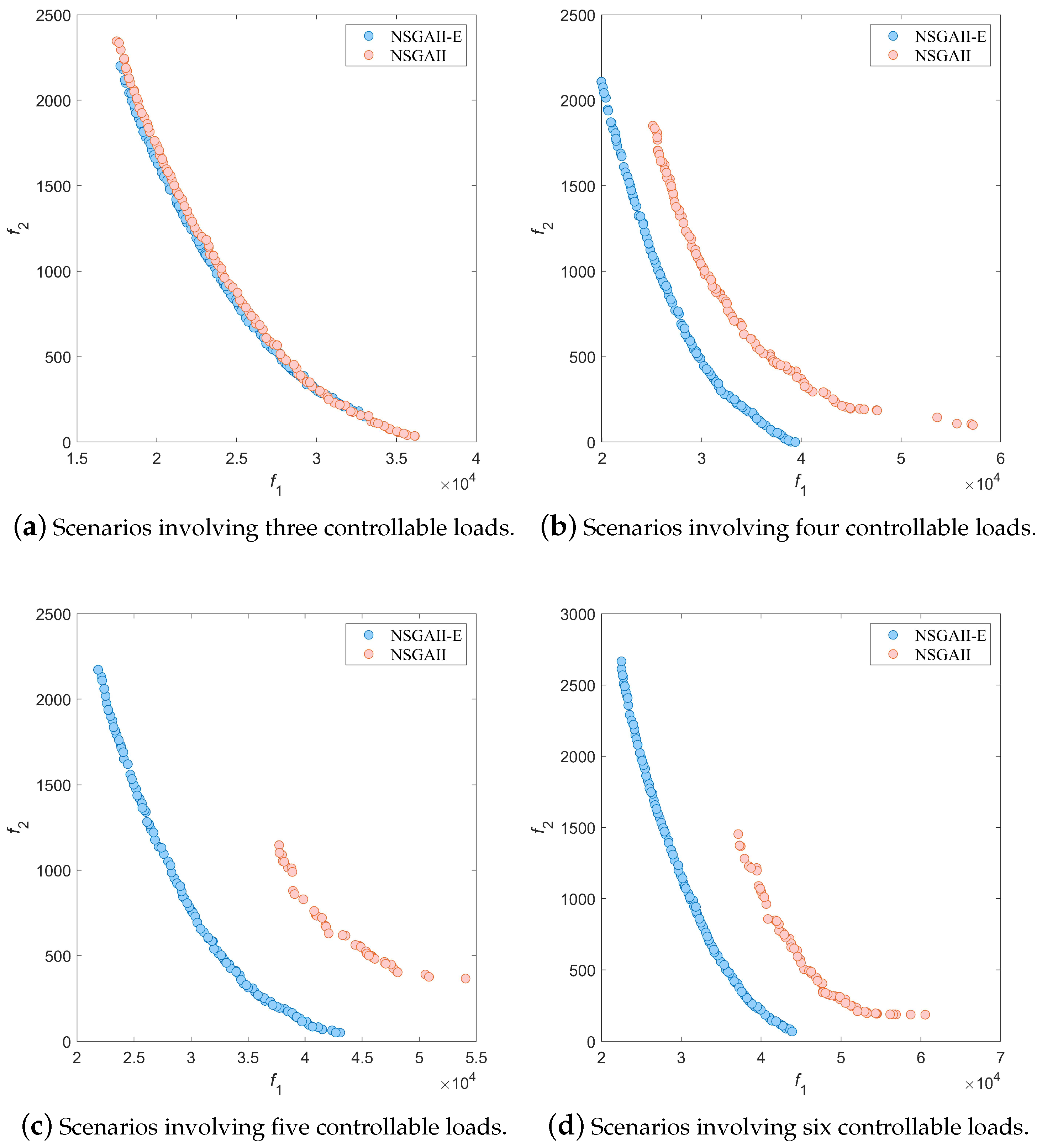
Furthermore, Figure 2 provides a comparison of the Pareto fronts between NSGA-II-MC and the traditional NSGA-II under different scenarios. The optimization objectives in the problems are minimizing operating costs and reducing dependence on the power grid. Each point on the Pareto front represents a management solution, with the horizontal and vertical axes representing the values of the two objective functions. Therefore, points closer to the origin indicate better convergence (optimality) of the algorithm. Multi-objective optimization also considers the diversity of the Pareto front, which involves how well a series of solutions can cover different objective preferences. This is reflected in the distribution of the Pareto front formed by a series of solutions. A more evenly distributed Pareto front that covers a wider range of objective values indicates better diversity. This means that more choices can be provided to decision-makers.

The results from Figure 2 demonstrate that the NSGA-II-MC algorithm proposed in this paper exhibits significant advantages over the traditional NSGA-II algorithm, showcasing improved convergence and diversity. It is worth noting that in the scenario with three controllable loads, the algorithm proposed in this paper shows a relatively smaller advantage. However, as the complexity of the management decision problem increases, i.e., with an increasing number of loads to be scheduled, the traditional NSGA-II algorithm struggles to reliably optimize the problem. In contrast, the NSGA-II-MC algorithm designed in this paper demonstrates superior performance. In the scenario with six controllable loads, there is a noticeable gap between NSGA-II-MC and NSGA-II. As the problem scale increases and constraint complexity grows, the advantages of the NSGA-II-MC algorithm become more pronounced. This validates the effectiveness and reliability of the multi-objective optimization approach proposed in this paper.

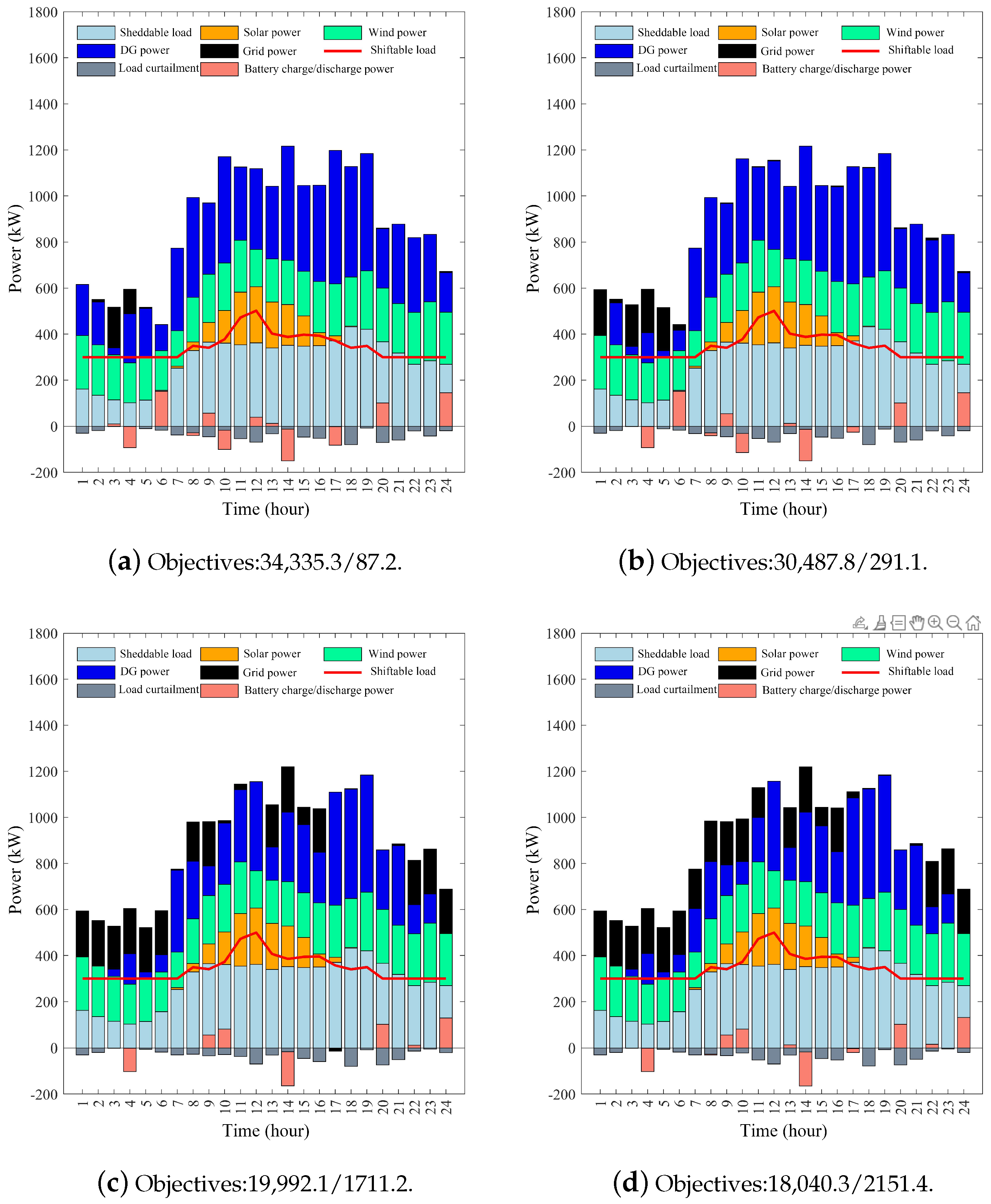
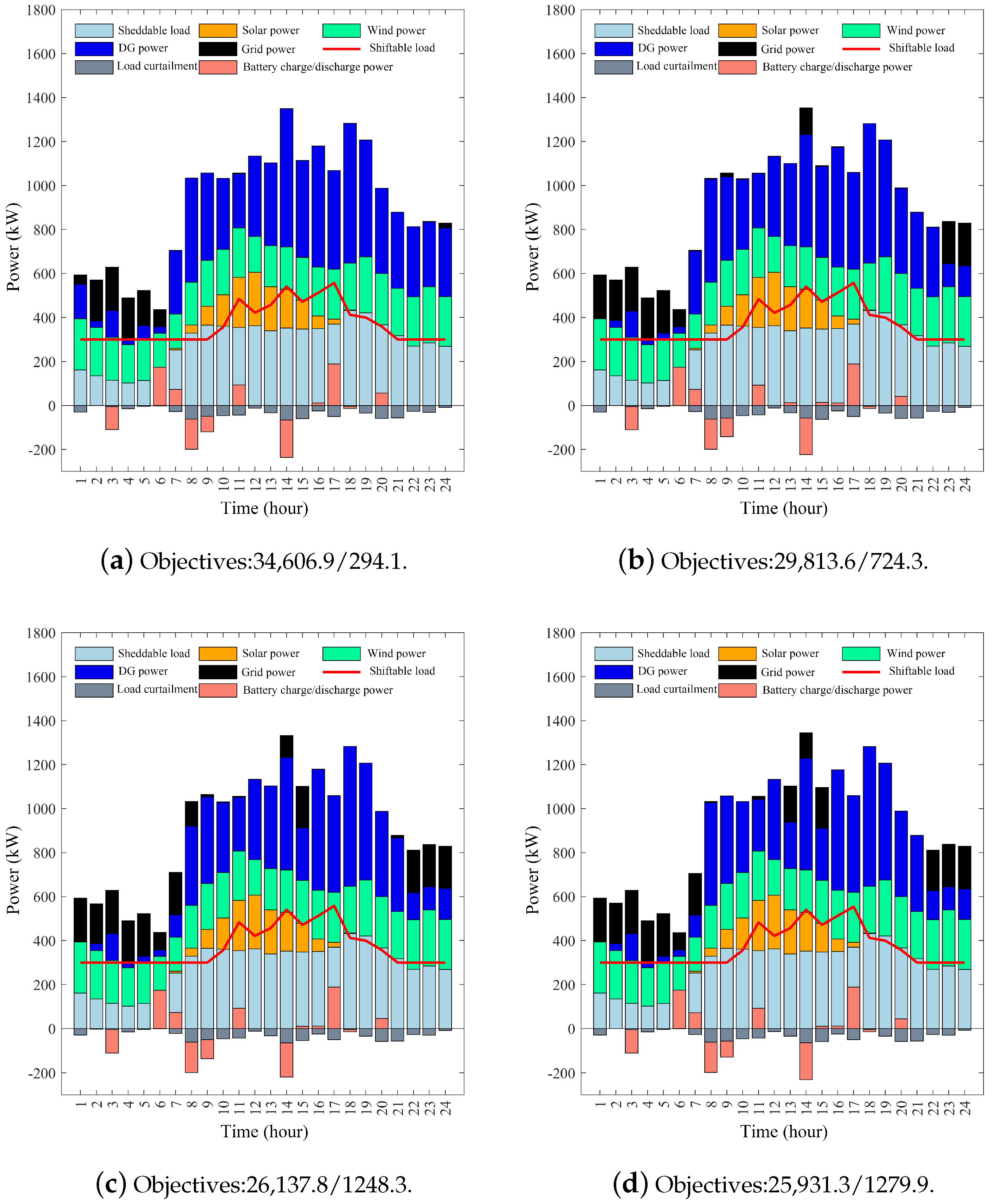
Figure 3 presents the management strategies under different objective preferences with three controllable loads, where (a–d) represent the strategies under various objective preferences. Objective one is the total cost, and objective two is the dependence on the main grid. The management strategy charts display the power generation, load power, charging and discharging states of energy storage batteries, regulation states of controllable loads, and the shedding of switchable loads at different times. Here, the black bar chart represents the power supply from the main grid, the light blue bar chart indicates the power of switchable loads, the light yellow bar chart shows the photovoltaic power generation, the green bar chart depicts the wind power generation, the blue bar chart is for the diesel engine’s power generation, the red line chart represents the regulation power of controllable loads (including critical loads), the grey bar chart shows the power shedding of switchable loads, and the pink bar chart represents the battery’s charging and discharging power. Positive values for the main grid power supply and battery discharging indicate power supply to the system/battery discharge, and negative values indicate selling power to the main grid/battery charging.

From the results in Figure 3, it is evident that the management strategies under different objective preferences have significant differences. Strategy (a) represents the management strategy under the lowest dependence on the main grid, with the main grid supply power being noticeably the lowest and the grid dependence amounting to only USD 87.2 (for uniform comparison, all costs are calculated in U.S. dollars), but the system’s electricity cost is USD 34,335.3, indicating that the system is primarily powered by diesel generation, renewable generations, and energy storage batteries. However, because the diesel generator’s cost of generation is significantly higher than the electricity cost from the main grid, this leads to a noticeable increase in the system’s total electricity cost. Conversely, strategy (d) shows a significant increase in the main grid supply power, with grid dependence at USD 2151.4 but at a considerably reduced cost (USD 18,040.3), indicating that utilizing relatively cheaper main grid supply can effectively reduce system costs, albeit at the expense of significant dependence on the main grid.

The renewable energy generation situation under strategy (a) shows that around midnight, when photovoltaic cannot generate electricity and wind power is also low, but the base’s critical loads still need to run, the designed algorithm prioritizes power supply from the main grid, followed by energy storage battery supply to meet the demand of critical loads; around noon, when renewable energy sources like photovoltaic and wind have sufficient generation and load demand decreases, the algorithm charges the energy storage battery to meet the potential high load demand later, showing the rationality of the method. It is worth noting that strategies (a) and (d) are the first and last on the Pareto front, representing management strategies under a single-objective preference, while (b) and (c) are two randomly selected strategies from the middle of the Pareto front, representing management strategies considering a balance between the two objectives. Therefore, it can be seen that the multi-objective optimization method designed in this paper can provide multiple management strategies under different objective preferences in a single run, thereby offering various choices for decision-makers, dynamically managing the system’s energy storage, generation, load shedding, and load scheduling based on the available external power supply conditions.

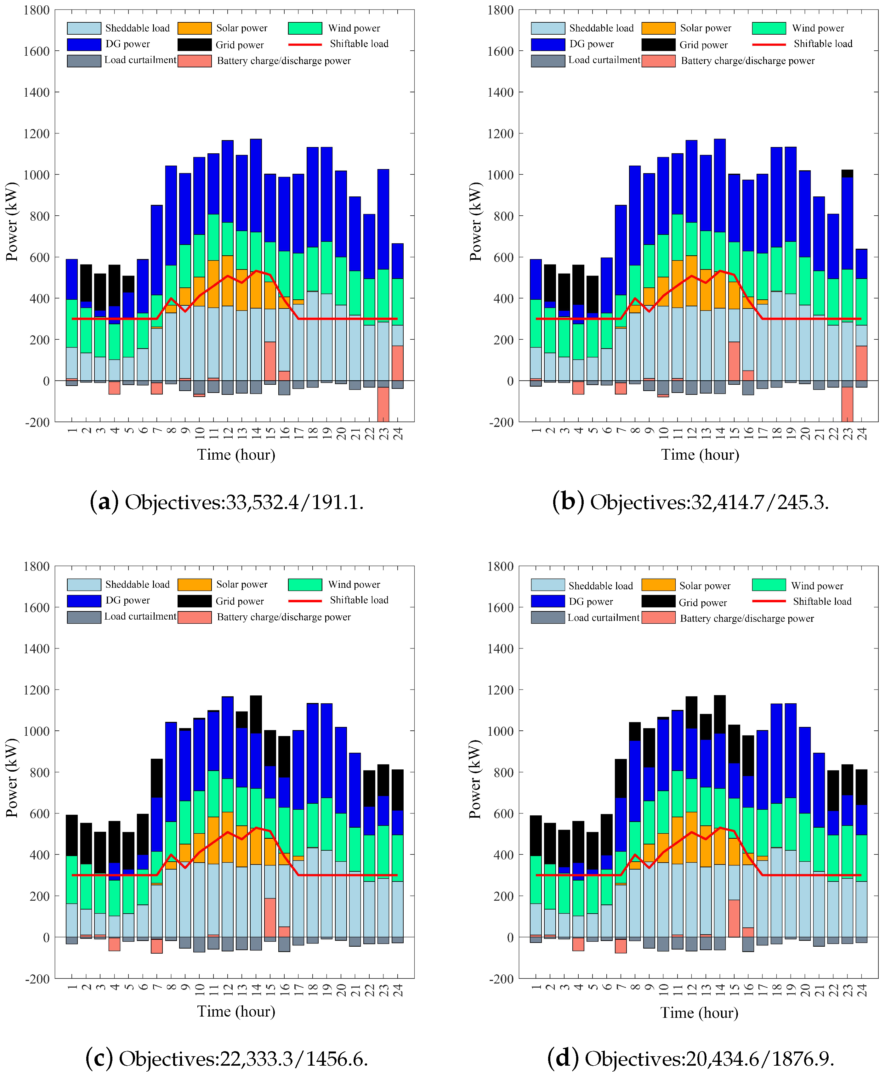
Figure 4 displays the management strategies under different objective preferences with four controllable loads, where (a–d) represent the strategies under various objective preferences. Compared to the scenario with three controllable loads shown in Figure 3, the addition of one more controllable load significantly changes the system’s management mode. During the peak energy demand period of critical and controllable loads from 13:00 to 15:00, the management algorithm designed in this paper tends to ensure energy balance by supplying power through the energy storage system and shedding loads to meet the system’s electricity demand. In the low-grid-dependence mode shown in (a), there is no need for grid power supply during this period, and the electricity demand shortfall is compensated by using diesel generators; in the low-operational cost-mode shown in (d), cost savings are achieved by supplying power through the main grid during this period. Due to the high cost of generation, diesel generators serve as a supplementary energy source at different times to address the issue of insufficient power from the energy storage batteries and renewable energy sources to meet electricity demand.

Figure 5 illustrates the management strategies under different objective preferences with five controllable loads, where (a–d) represent the strategies under various objective preferences. Compared to the scenarios with three and four controllable loads discussed above, the utilization rate of energy storage batteries significantly increases in this scenario due to the higher number of load demands, requiring frequent adjustments among various power supply resources. In the period from 22:00 to 24:00, with the same total load demand, the low-grid-dependence mode shown in (a) fulfills the system’s electricity needs using diesel generators, while scenarios (b–d), depending on their respective management modes and preferences for grid dependence, supply electricity demands from the main grid in varying proportions, demonstrating the algorithm’s rationality.

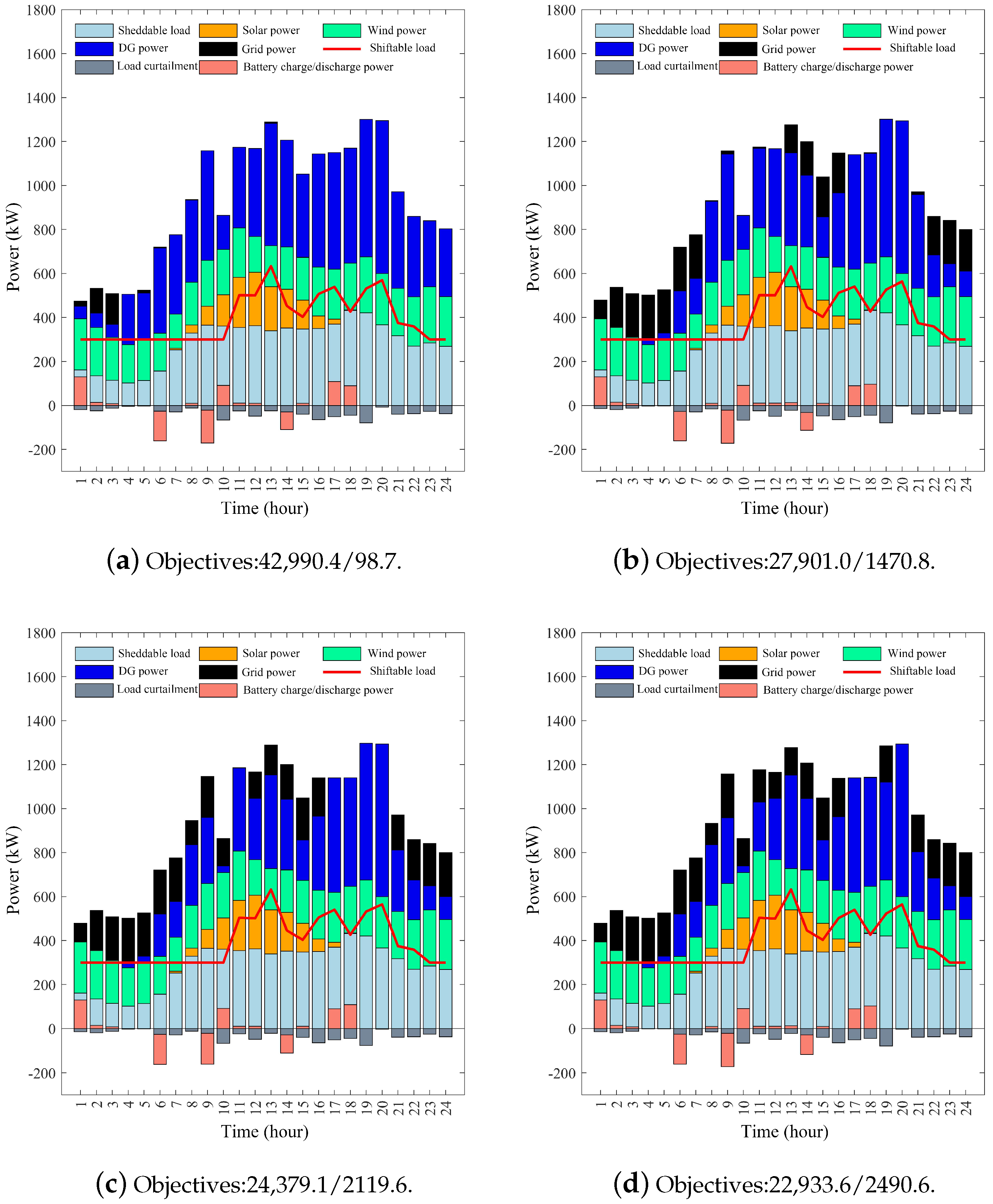
Figure 6 presents the management strategies under different objective preferences with six controllable loads. In scenarios with multiple controllable loads, the complexity of the system increases, leading inevitably to higher overall operational costs and greater dependence on the main grid. From the scenario operation diagrams, it can be observed that the addition of controllable loads creates a peak electricity demand period from 19:00 to 20:00. In the low-grid-dependence management mode (a), the algorithm exclusively uses diesel generators for power supply, resulting in high operational costs of USD 42,990.4. In contrast, management mode (d), which utilizes electricity from the main grid, can effectively reduce system costs.

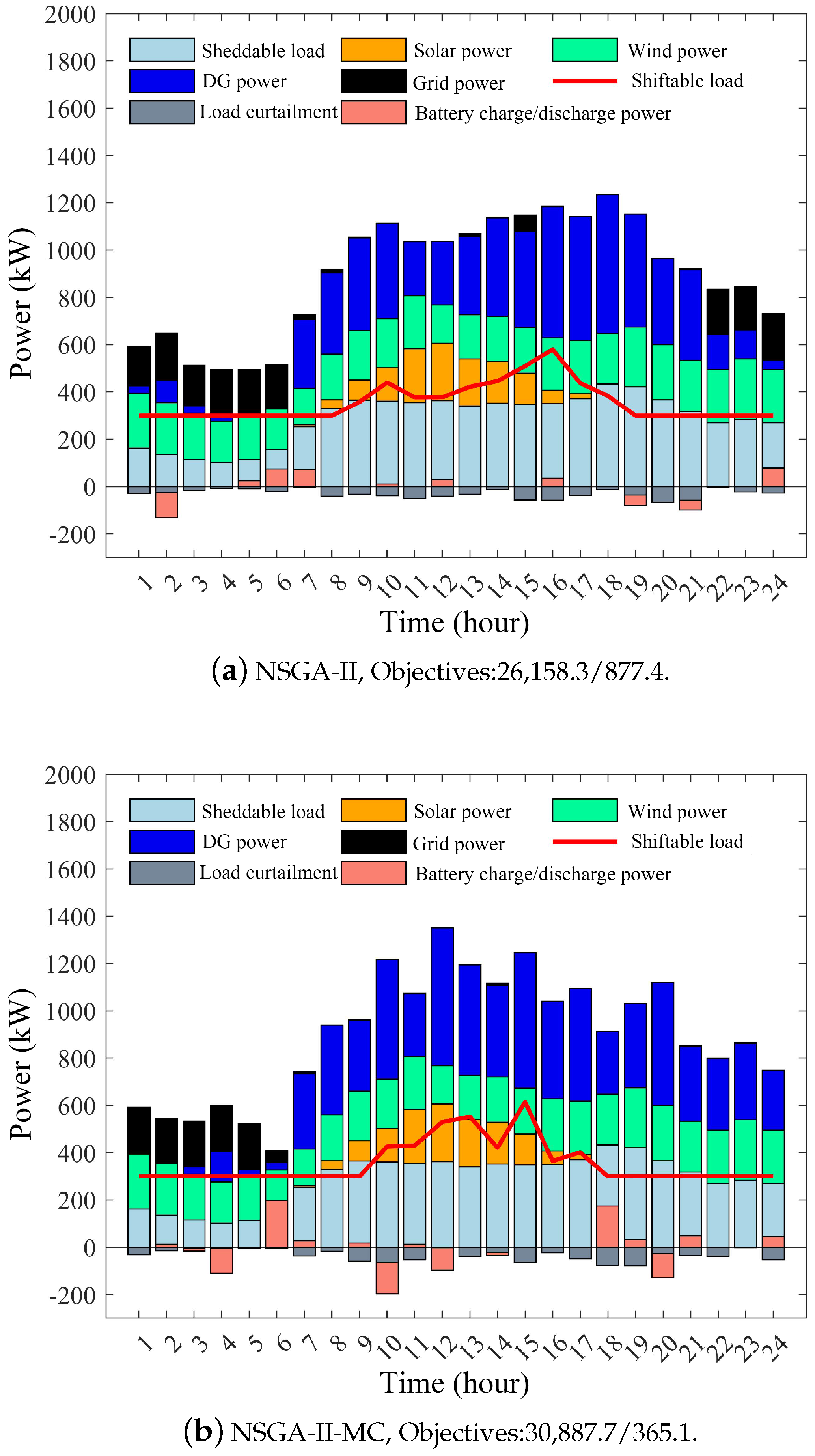
In addition, Figure 7 shows the comparative results of management strategies under four controllable loads scenarios between the NSGA-II-MC and NSGA-II algorithms. This experiment selected the solutions at the bottom of the Pareto front, i.e., the scenarios with the lowest dependency on the main grid. However, it can be seen from the results that the traditional NSGA-II algorithm struggles to meet this preference, still relying heavily on the main grid for power supply, whereas the NSGA-II-MC algorithm tends towards using diesel generators, better satisfying user preferences.

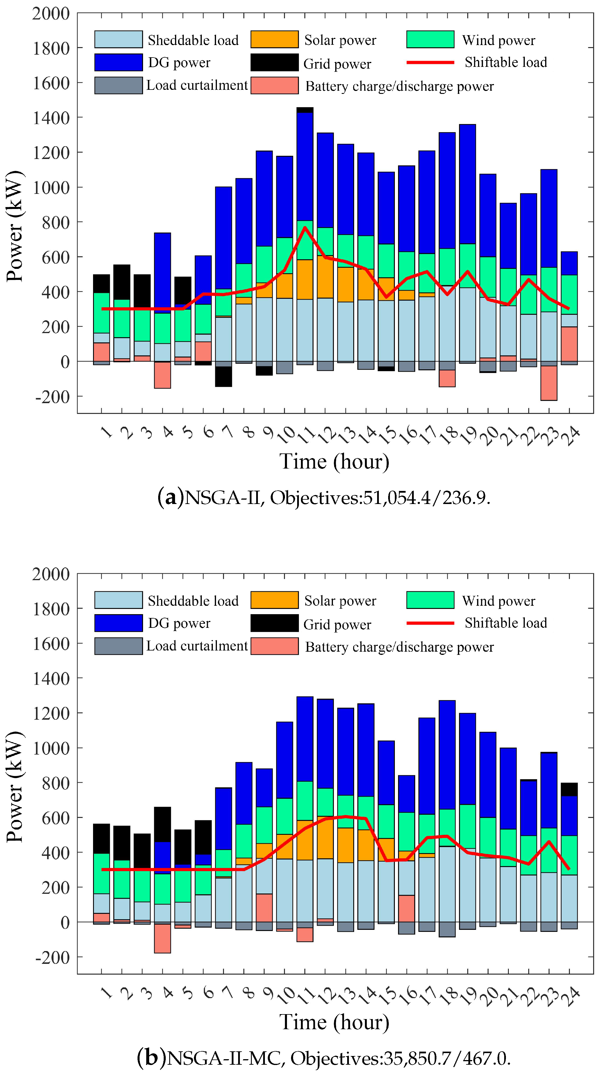
Figure 8 presents the comparison of management strategies between the NSGA-II-MC and NSGA-II algorithms under scenarios with six controllable loads. Comparing the objective values of the two solutions reveals that, in the complex management scenario of six controllable loads, the NSGA-II algorithm struggles to achieve effective optimization, with operational costs reaching USD 51,054.4. Meanwhile, the management strategy derived from the NSGA-II-MC algorithm can achieve a reduction of more than USD 16,000 in operational costs with only about 200 increases in dependency level, demonstrating a clear advantage in algorithm convergence.

The results above indicate that the multi-objective optimization method proposed in this paper can intelligently generate management strategies for resilient microgrids with different objective preferences. With a single run, it is possible to obtain management plans with varying degrees of grid dependence. For example, in a military base, management modes with low grid dependence are suitable for wartime energy system management, while those with low operational costs are suitable for the economical operation of energy systems during peacetime. Furthermore, the results demonstrate that the traditional NSGA-II algorithm had difficulty meeting various preferences and failed to converge under stringent constraints, resulting in high costs and substantial reliance on the grid. In contrast, the proposed NSGA-II-MC algorithm can efficiently manage these constraints and generate satisfactory energy management solutions tailored to diverse preferences.

5. Conclusions

This paper introduces a multi-stage constraint-handling multi-objective optimization method specifically designed for resilient microgrid energy management. Managing complex controls of generators, batteries, switchable loads, and controllable loads presents challenging constraints that the management strategy must meet. The multi-stage constraint-handling approach is developed to address these challenges effectively. Compared to conventional multi-objective optimization methods, our proposed method demonstrates superior performance to nine state-of-the-art methods, exhibiting the best convergence and diversity in the obtained Pareto front. The multi-objective optimization method presented in this study can intelligently generate management strategies catering to different objective preferences. In just a single run, it can produce management plans that vary in their degree of grid dependence. However, the model does not account for data uncertainty in the microgrid system. Moreover, it assumes that the predicted wind and solar power outputs are perfectly accurate, which is not the case in actual predictions due to inherent errors. Therefore, future research should consider the inaccuracies present in renewable energy forecasts and incorporate factors of uncertainty into the analysis. In addition, future research could expand the proposed method to more complex microgrid systems or to scenarios involving multiple microgrids.

References

1. Javidsharifi, M.; Niknam, T.; Aghaei, J.; Mokryani, G. Multi-objective short-term scheduling of a renewable-based microgrid in the presence of tidal resources and storage devices. Appl. Energy 2018, 216, 367–381. [Google Scholar] [CrossRef]
2. Zhang, Y.; Gatsis, N.; Giannakis, G.B. Robust energy management for microgrids with high-penetration renewables. IEEE Trans. Sustain. Energy 2013, 4, 944–953. [Google Scholar] [CrossRef]
3. Liu, G.; Xu, Y.; Tomsovic, K. Bidding strategy for microgrid in day-ahead market based on hybrid stochastic/robust optimization. IEEE Trans. Smart Grid 2015, 7, 227–237. [Google Scholar] [CrossRef]
4. Badawy, M.O.; Sozer, Y. Power flow management of a grid tied PV-battery system for electric vehicles charging. IEEE Trans. Ind. Appl. 2016, 53, 1347–1357. [Google Scholar] [CrossRef]
5. Tanvir, A.A.; Merabet, A. Artificial neural network and Kalman filter for estimation and control in standalone induction generator wind energy DC microgrid. Energies 2020, 13, 1743. [Google Scholar] [CrossRef]
6. Roy, K.; Mandal, K.K.; Mandal, A.C. Energy management system of microgrids in grid-tied mode: A hybrid approach. Energy Sources Part A Recover. Util. Environ. Eff. 2022, 1–23. [Google Scholar] [CrossRef]
7. Li, X.; Wang, S. Energy management and operational control methods for grid battery energy storage systems. CSEE J. Power Energy Syst. 2019, 7, 1026–1040. [Google Scholar]
8. Pannala, S.; Patari, N.; Srivastava, A.K.; Padhy, N.P. Effective control and management scheme for isolated and grid connected DC microgrid. IEEE Trans. Ind. Appl. 2020, 56, 6767–6780. [Google Scholar] [CrossRef]
9. de Oliveira-Assis, L.; García-Trivino, P.; Soares-Ramos, E.P.; Sarrias-Mena, R.; García-Vázquez, C.A.; Ugalde-Loo, C.E.; Fernández-Ramírez, L.M. Optimal energy management system using biogeography based optimization for grid-connected MVDC microgrid with photovoltaic, hydrogen system, electric vehicles and Z-source converters. Energy Convers. Manag. 2021, 248, 114808. [Google Scholar] [CrossRef]
10. Zhao, Z.; Guo, J.; Luo, X.; Lai, C.S.; Yang, P.; Lai, L.L.; Li, P.; Guerrero, J.M.; Shahidehpour, M. Distributed robust model predictive control-based energy management strategy for islanded multi-microgrids considering uncertainty. IEEE Trans. Smart Grid 2022, 13, 2107–2120. [Google Scholar] [CrossRef]
11. Merabet, A.; Al-Durra, A.; El-Saadany, E.F. Energy management system for optimal cost and storage utilization of renewable hybrid energy microgrid. Energy Convers. Manag. 2022, 252, 115116. [Google Scholar] [CrossRef]
12. Nammouchi, A.; Aupke, P.; D’andreagiovanni, F.; Ghazzai, H.; Theocharis, A.; Kassler, A. Robust opportunistic optimal energy management of a mixed microgrid under asymmetrical uncertainties. Sustain. Energy Grids Netw. 2023, 36, 101184. [Google Scholar] [CrossRef]
13. Chen, H.; Gao, L.; Zhang, Z. Multi-objective optimal scheduling of a microgrid with uncertainties of renewable power generation considering user satisfaction. Int. J. Electr. Power Energy Syst. 2021, 131, 107142. [Google Scholar] [CrossRef]
14. Rui, T.; Li, G.; Wang, Q.; Hu, C.; Shen, W.; Xu, B. Hierarchical optimization method for energy scheduling of multiple microgrids. Appl. Sci. 2019, 9, 624. [Google Scholar] [CrossRef]
15. Vidan, M.; D’Andreagiovanni, F.; Pandžić, H. Individual thermal generator and battery storage bidding strategies based on robust optimization. IEEE Access 2021, 9, 66829–66838. [Google Scholar] [CrossRef]
16. Li, X.; Xia, R. A dynamic multi-constraints handling strategy for multi-objective energy management of microgrid based on MOEA. IEEE Access 2019, 7, 138732–138744. [Google Scholar] [CrossRef]
17. Roselyn, J.P.; Devaraj, D.; Dash, S.S. Multi-Objective Genetic Algorithm for voltage stability enhancement using rescheduling and FACTS devices. Ain Shams Eng. J. 2014, 5, 789–801. [Google Scholar] [CrossRef]
18. Murty, V.; Kumar, A. RETRACTED ARTICLE: Multi-objective energy management in microgrids with hybrid energy sources and battery energy storage systems. Prot. Control Mod. Power Syst. 2020, 5, 1–20. [Google Scholar] [CrossRef]
19. Li, M.; Wang, L.; Wang, Y.; Chen, Z. Sizing Optimization and Energy Management Strategy for Hybrid Energy Storage System Using Multiobjective Optimization and Random Forests. IEEE Trans. Power Electron. 2021, 36, 11421–11430. [Google Scholar] [CrossRef]
20. De, M.; Mandal, K.K. Energy management strategy and renewable energy integration within multi-microgrid framework utilizing multi-objective modified personal best particle swarm optimization. Sustain. Energy Technol. Assess. 2022, 53, 102410. [Google Scholar] [CrossRef]
21. Li, Y.; Wang, P.; Gooi, H.B.; Ye, J.; Wu, L. Multi-objective optimal dispatch of microgrid under uncertainties via interval optimization. IEEE Trans. Smart Grid 2017, 10, 2046–2058. [Google Scholar] [CrossRef]
22. Rajagopalan, A.; Nagarajan, K.; Montoya, O.D.; Dhanasekaran, S.; Kareem, I.A.; Perumal, A.S.; Lakshmaiya, N.; Paramasivam, P. Multi-objective optimal scheduling of a microgrid using oppositional gradient-based grey wolf optimizer. Energies 2022, 15, 9024. [Google Scholar] [CrossRef]
23. Aghajani, G.; Ghadimi, N. Multi-objective energy management in a micro-grid. Energy Rep. 2018, 4, 218–225. [Google Scholar] [CrossRef]
24. Sarshar, J.; Moosapour, S.S.; Joorabian, M. Multi-objective energy management of a micro-grid considering uncertainty in wind power forecasting. Energy 2017, 139, 680–693. [Google Scholar] [CrossRef]
25. Mansouri, S.A.; Ahmarinejad, A.; Nematbakhsh, E.; Javadi, M.S.; Jordehi, A.R.; Catalao, J.P. Energy management in microgrids including smart homes: A multi-objective approach. Sustain. Cities Soc. 2021, 69, 102852. [Google Scholar] [CrossRef]
26. Zhai, M.; Liu, Y.; Zhang, T.; Zhang, Y. Robust model predictive control for energy management of isolated microgrids. In Proceedings of the 2017 IEEE International Conference on Industrial Engineering and Engineering Management (IEEM), Singapore, 10–13 December 2017; IEEE: Piscataway, NJ, USA, 2017; pp. 2049–2053. [Google Scholar]
27. Hong, T.; Pinson, P.; Fan, S.; Zareipour, H.; Troccoli, A.; Hyndman, R.J. Probabilistic energy forecasting: Global energy forecasting competition 2014 and beyond. Int. J. Forecast. 2016, 32, 896–913. [Google Scholar] [CrossRef]
28. Panichella, A. An adaptive evolutionary algorithm based on non-Euclidean geometry for many-objective optimization. In Proceedings of the GECCO’19: Genetic and Evolutionary Computation Conference, Prague, Czech Republic, 13–17 July 2019; pp. 595–603. [Google Scholar]
29. Jain, H.; Deb, K. An evolutionary many-objective optimization algorithm using reference-point based nondominated sorting approach, part II: Handling constraints and extending to an adaptive approach. IEEE Trans. Evol. Comput. 2013, 18, 602–622. [Google Scholar] [CrossRef]
30. Tian, Y.; Cheng, R.; Zhang, X.; Cheng, F.; Jin, Y. An indicator-based multiobjective evolutionary algorithm with reference point adaptation for better versatility. IEEE Trans. Evol. Comput. 2017, 22, 609–622. [Google Scholar] [CrossRef]
31. Tian, Y.; Zhang, T.; Xiao, J.; Zhang, X.; Jin, Y. A coevolutionary framework for constrained multiobjective optimization problems. IEEE Trans. Evol. Comput. 2020, 25, 102–116. [Google Scholar] [CrossRef]
32. Li, K.; Chen, R.; Fu, G.; Yao, X. Two-archive evolutionary algorithm for constrained multiobjective optimization. IEEE Trans. Evol. Comput. 2018, 23, 303–315. [Google Scholar] [CrossRef]
33. Jiao, R.; Zeng, S.; Li, C.; Yang, S.; Ong, Y.S. Handling constrained many-objective optimization problems via problem transformation. IEEE Trans. Cybern. 2020, 51, 4834–4847. [Google Scholar] [CrossRef] [PubMed]
34. Deb, K.; Pratap, A.; Agarwal, S.; Meyarivan, T. A fast and elitist multiobjective genetic algorithm: NSGA-II. IEEE Trans. Evol. Comput. 2002, 6, 182–197. [Google Scholar] [CrossRef]
35. Deb, K.; Jain, H. An evolutionary many-objective optimization algorithm using reference-point-based nondominated sorting approach, part I: Solving problems with box constraints. IEEE Trans. Evol. Comput. 2013, 18, 577–601. [Google Scholar] [CrossRef]
36. Cheng, R.; Jin, Y.; Olhofer, M.; Sendhoff, B. A reference vector guided evolutionary algorithm for many-objective optimization. IEEE Trans. Evol. Comput. 2016, 20, 773–791. [Google Scholar] [CrossRef]
37. Tian, Y.; Cheng, R.; Zhang, X.; Jin, Y. PlatEMO: A MATLAB Platform for Evolutionary Multi-Objective Optimization. IEEE Comput. Intell. Mag. 2017, 12, 73–87. [Google Scholar] [CrossRef]
Figure 1. The actual proportion of feasible solutions does not change as expected.
Applsci 14 03253 g001
Figure 2. Comparison of the Pareto Fronts between the NSGA-II-MC Algorithm and Traditional Algorithms in Different Scenarios.
Applsci 14 03253 g002
Figure 3. Management strategies under different objective preferences with three controllable loads.
Applsci 14 03253 g003
Figure 4. Management strategies under different objective preferences with four controllable loads.
Applsci 14 03253 g004
Figure 5. Management strategies under different objective preferences with five controllable loads.
Applsci 14 03253 g005
Figure 6. Management strategies under different objective preferences with six controllable loads.
Applsci 14 03253 g006
Figure 7. Comparison of NSGA-II-MC and NSGA-II management strategies (four controllable loads).
Applsci 14 03253 g007
Figure 8. Comparison of NSGA-II-MC and NSGA-II management strategies (six controllable loads).
Applsci 14 03253 g008