Structural Detection and Stability Monitoring of Deep Strata on a Slope Using High-Density Resistivity Method and FBG Strain Sensors

Abstract

Under the influence of a variety of unfavorable factors, slope instability may occur, so the stability of the slope needs to be analyzed. In this paper, combined with the geological investigation data, the slope engineering geological profiles are derived based on 2D inversion maps of the high-density resistivity (HDR) method to obtain the overburden layer thickness. Then, a finite element model is established based on the mechanical and geometric parameters of the slope to analyze the displacement and deformation characteristics and obtain information about the potential sliding surface. The above analysis results are combined to determine the effective monitoring field and deploy (Fiber Bragg Grating) FBG strain detection piles for deep strain monitoring. The analysis showed that the shape and location of the potential sliding surface of the slope from the numerical simulation are consistent with those delineated by the HDR profile. The monitoring results show the rock and soil on the north side of the slope are soft and have poor stability, which is consistent with the HDR method detection results. Adopting the HDR method to identify the slope’s overall geological structure combined with FBG strain detection piles to obtain the deep deformation provided an effective monitoring technique for slope stability assessment.

1. Introduction

Slope instability is often triggered and aggravated under the influence of external unfavorable factors, which lead to the reduction in soil shear strength, causing shear stresses in the soil to be greater than the shear strength of the soil, resulting in sliding instability. Therefore, it is necessary to investigate and monitor the overall geological structure and deep deformation of the slope, analyze the deformation status of the soil, predict the trend of structural deformation, and carry out structural stability evaluation based on the deep strain monitoring data of the slope.

The high-density resistivity (HDR) method is widely adopted [1,2,3] as an engineering geophysical exploration method to investigate the deep geological structures of slopes. Zhuo Jia et al. [4] introduced the basic principle, data processing, result explanation and inference of the HDR method and applied it to the slope of the Gongchangling open pit mine to deeply investigate the physical parameters, such as resistivity and thickness, of the geological body of the slope to determine the stability of the slope. Hu et al. [5] combined high-density resistivity (HDR), ground-penetrating radar (GPR), and geological drilling methods to determine the stratigraphic distribution of the Beian-Heihe Highway region. Wu et al. [6] studied the subsurface features of Ordos using the transient electromagnetic method (TEM) and HDR method to identify the coal mining void areas based on rock resistivity distribution. S. Szalai et al. [7] studied a slowly moving loess slope using the HDR method to identify its mechanically weak areas, predict future rupture surfaces, and depict the danger zones. Chen et al. [8] used the high-density electrical method to detect the landslide body in Xiaozhuang Village, Changjiahe Town, to explore the stratigraphic structure, thickness of the landslide body, groundwater distribution, and spatial spreading of the landslide area. Wang et al. [9] used the high-density electrical method to detect a typical loess seismic landslide in the southwestern mountainous area of Xiji County, Ningxia, then verified and analyzed it with drilling data to identify the characteristics of the stratigraphic structure, loess thickness, bedrock burial depth, water-rich section, and spatial spreading in the landslide area. Gan et al. [10] used the HDR method to probe the overburden thickness, karst cavities, and sliding zone locations in the mine area of Nanhengzhen to delineate the stratigraphic lithology and limestone distribution zones. Oladunjoye P. Olabode et al. [11] carried out HDR measurements on weathered basal slopes of medium and fine-grained granitic rocks in the Sungai Ara area of the Penang hills, and six HDR profiles were obtained at different elevations of the slope sites. Chen et al. [12] performed a geophysical survey combined with seismic refraction tomography (SRT), seismic scattered wave imaging (SSI), and high-density resistivity (HDR) along five profiles over the landslide body. Liu and Yang [13] used the Wenner device to detect the slope of Huangming Reservoir in Yuyao City, analyze the weathering degree of rock, and evaluate the stability of the slope. Hruška et al. [14] used GPR and HDR geophysical methods to probe the slope at different times and observed changes in the geophysical profiles over time. The results demonstrated the processes where a significant expansion of wet areas inside both studied rock masses is associated with the logging operations. Lu et al. [15] used the HDR method to detect the Baijiabao landslide and derived the water content based on the inversion of the resistivity model. Kang et al. designed [16] a physical model of a rainfall-affected slope and used the HDR method to measure the apparent resistivity of the slope rock and soil mass at different rainfall times to analyze the formation process of internal disaster sources of the rainfall-affected slope.

Physical detection methods, such as HDR and GPR, can identify geological structures and help preliminarily determine the engineering geological structure of slope rock and soil mass. Based on an analysis of the overall geologic structure of the slope, sensors buried inside the slope can continuously monitor the movement of the geotechnical mass and provide dynamic monitoring data over time.

In recent years, FBG sensors have been widely applied in the field of geotechnical engineering because of their ability to resist electromagnetic interference, high accuracy, online monitoring, and multiplexing compared to traditional sensors. Many researchers [17,18] have combined borehole-based deep displacement monitoring methods with FBG strain sensors for slope stability monitoring. Yoshida et al. [19] developed a monitoring system with a borehole inclinometer using FBG as a strain sensor to monitor artificial slope deformation for four months during the construction term. The monitoring system worked properly and the availability of the FBG borehole inclinometer was proved. Pei et al. [20] present a monitoring system consisting of FBG-based in-place inclinometers for monitoring movements of landslides and have installed the FBG-based in-place inclinometers at a site in Weijiagou Valley, China. Guo et al. [21] proposed an easy-mounting sensor structure containing several inclinometer casings and a series of flexible pipes with FBGs connected to each other. The FBG deformation sensors have been installed in a slope, and a matched monitoring station has been established and operated. Zhang et al. [22] employed Integrated Fiber Optical Sensing Technology (IFOST) to test the surface as well as the deep deformation of the slope by embedding the sensing fibers into the soil by boreholes. Huang et al. [23] developed a series of FBG-based transducers that include inclination, linear displacement, and differential pore pressure sensors for comprehensive evaluation of slope stability and presented cases of field monitoring using the FBG sensor arrays. Guo et al. [24] applied FBG technology in a traditional inclinometer, proposed a method to calculate displacement based on wavelength change, and used this method for the safety monitoring of the right side slope in the section ZK56 + 860~ZK56 + 940 of Longyong Expressway. Hu et al. [25] proposed a fiber Bragg grating-based monitoring and warning system for expressway slopes, and the four-level early warning method based on statistical analysis was introduced, characterized by four different displacement rate ranges. Zhang et al. [26] investigated internal deformation and the failure of a centrifuge model slope with horizontally and vertically embedded FBG arrays. Zhang et al. [27] designed a real-time monitoring system based on FBG technology for the Majiagou landslide, which records the displacement at the deeper sliding surface, together with the rainfall, water level, pore water pressure, and temperature, and according to the analysis of these data, the stability evaluation of the slope was carried out. Zheng et al. [28] designed an inclinometer using fiber Bragg grating to measure the internal displacement of the slope and carried out field monitoring suitability tests. Ren et al. [29] implemented a fiber Bragg grating (FBG) sensors array into the deep unconsolidated layer to realize long-term ground monitoring. Zeng et al. [30] fabricated an in-place FBG-based inclinometer to determine the deformation movement of a slope. Han et al. [31] embedded the ultra-weak fiber Bragg grating in the boreholes for monitoring and determined the range of plastic zone for each borehole according to the monitoring results.

In this paper, the engineering geological profiles were acquired based on 2D inversion maps of the high-density resistivity method combined with geologic exploration data to determine the location of potential sliding surfaces and areas of weakness. Then, the slope finite element numerical models were established to analyze the deformation and damage characteristics, and the location and shape of the sliding surface of the slope were obtained. Finally, the specific location of the monitoring system was confirmed based on the results of the above analysis, and the FBG strain detection piles were deployed to monitor the deformation of the deep stratigraphy.

2. Interpretation of Engineering Geologic Structures of Slope Based on 2-D Inversion Maps of High-Density Resistivity

The Yuanyang-Luchun Secondary Highway is located in the southwest of Honghe Prefecture, Yunnan Province, and runs from northeast to southwest, the geological working slope is situated between highway miles K77 + 120~K77 + 215. The slope is located south of the Tropic of Cancer and has a subtropical climate with no snow throughout the year; the average temperature for many years is 16.9°C~16.44 °C, respectively. The rainy season is mostly concentrated from May to September, with April, October, and November as the flat water period and the remaining four months as the dry season; the average precipitation over the years is 1450.89~2108.99 mm. The previous geological survey showed that the stratigraphy is composed of a Quaternary ($Q_4^{dl+el}$) slope residual layer, Triassic ($T_{3}g$) upper mudstone, and Indosinian diorite. The slope residual layer consists of yellow-brown clay and sandy clay with 20~40% gravel; the gravel is less than 6 cm in diameter, 5~7 cm thick, and composed of mudstone fragments and diorite fragments. The mudstone is purple-brown, with each layer 3~5 cm thick, and produces a crisp sound when struck with a hammer. Diorite is grayish-green or bluish-gray, with a hard and brittle texture. In weakly weathered conditions, it appears yellowish.

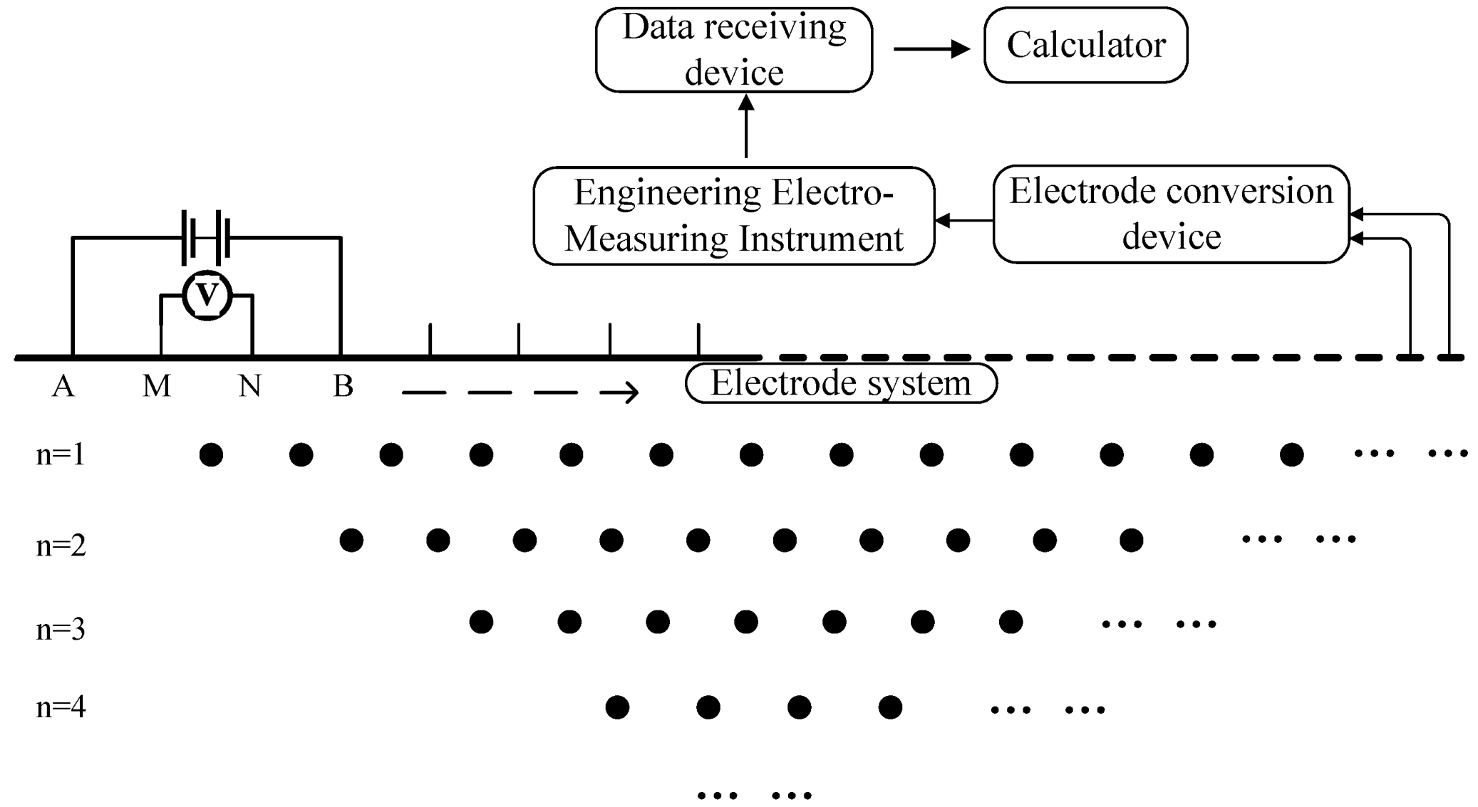
To obtain the overall geologic structure of the slope, the high-density resistivity (HDR) method was applied to investigate the slope. The HDR method is based on the differences in electrical conductivity of different rocks and soil, which studies the underground distribution law under the action of an artificially applied stable current field; the principle of operation is shown in Figure 1.

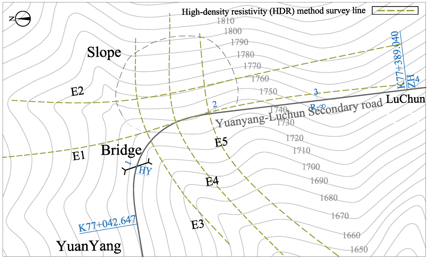
A, M, N, and B are arranged at equal intervals, the power supply electrodes are A and B, and the measuring electrodes are M and N; AM = MN = NB is an electrode distance. The electrode spacing was increased uniformly at equal intervals by the isolation factor. The four electrodes are moved together point by point in the direction of the survey line to obtain the first profile; then, the spacing between neighboring electrodes is increased, and measurements are continued to obtain the next profile line. Measurements are continued downward to obtain an inverted trapezoidal section. According to the detection requirements and area topography, the two cross-sectional survey lines (E1, E2) and three longitudinal-section survey lines (E3, E4, E5) were laid on the slope surface. The specific survey line arrangement is shown in Figure 2. Combined with the geological investigation data, we interpreted the high-density resistivity 2D inversion images into engineering geological profiles to analyze the overall geological structure of the slope.

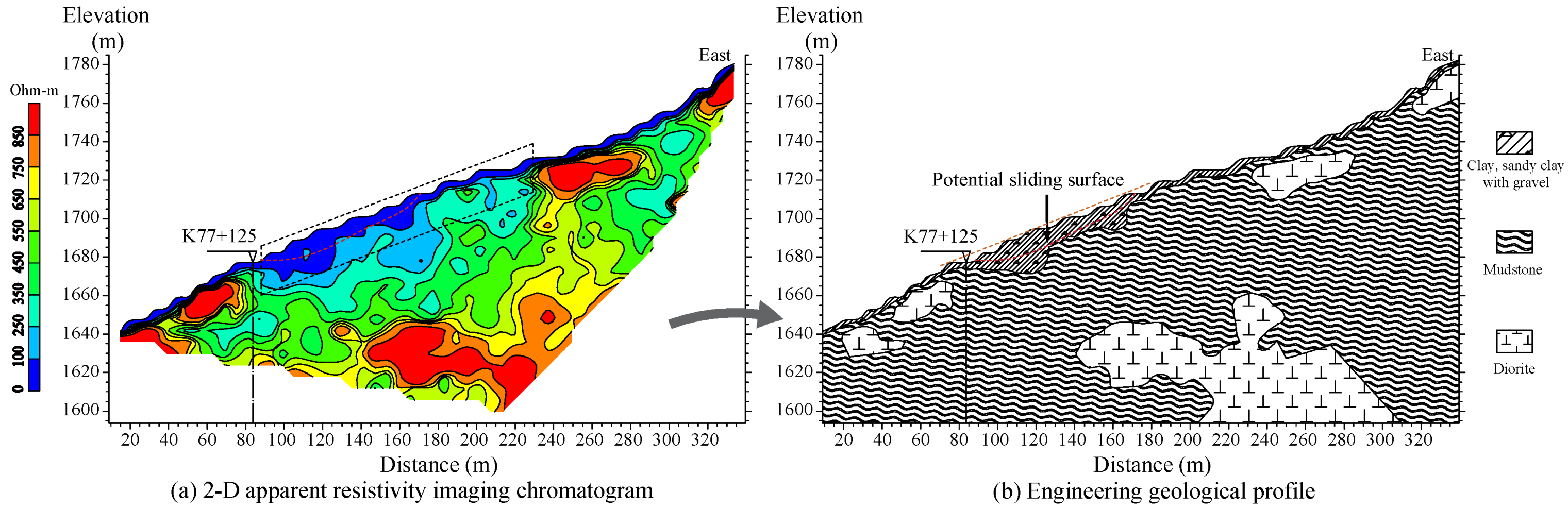
The apparent resistivity profile and the engineering geological profile of E1~E5 are shown in Figure 3, Figure 4, Figure 5, Figure 6 and Figure 7. The resistivity values range from 100~950 $\Omega$·m, and the distributions of underground rock formations are very irregular. 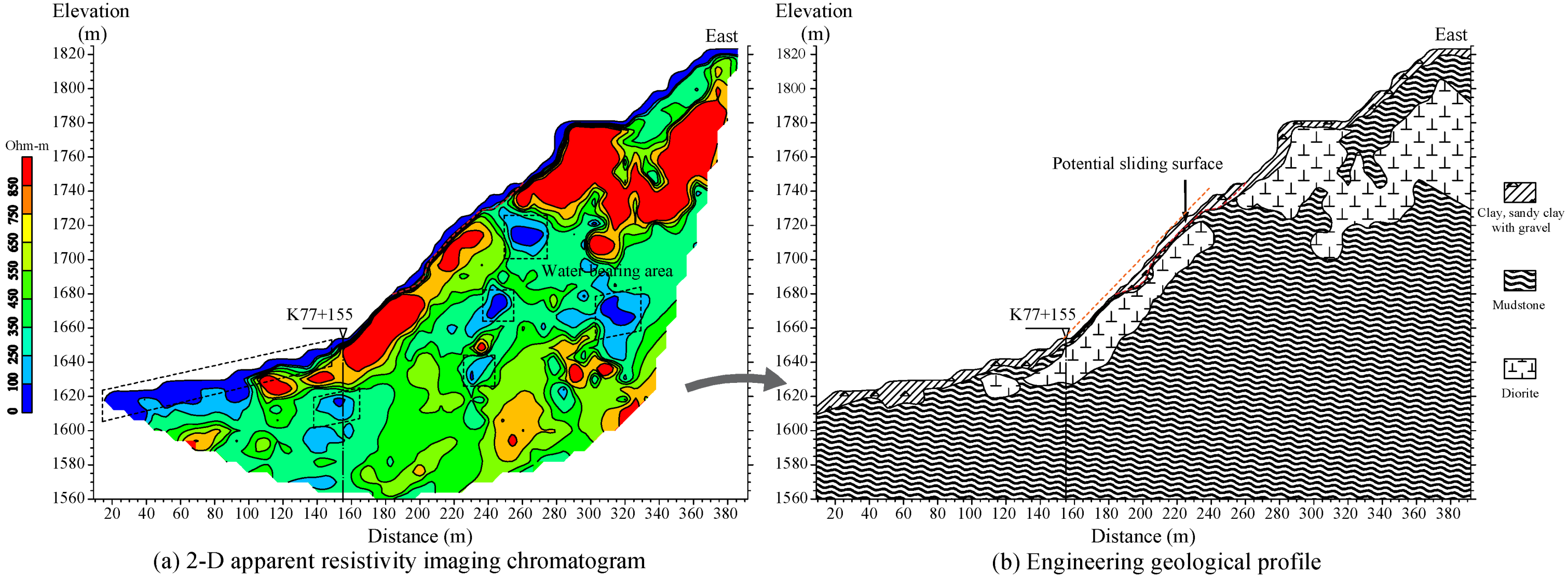The survey line E1 is located on the foundation of the highway, and the dark blue low-resistivity area in Figure 3 is a backfill soil layer, with a thickness of 10~15 m and a resistivity of about 100 $\Omega$·m. It is also the anti-slip section of the leading edge of the slope, i.e., the platform area, which is basically in a stable state. The survey line E2 is laid in the middle of the slope. The low-resistivity layer in the shallow surface layer in Figure 4 is the slope residual layer, with an apparent resistivity of 100 $\Omega$·m, which is mainly composed of clay and sandy clay, with a thickness of 2~5 m. It is shown in Figure 4 that the magmatic intrusion activity is strong, resulting in a very irregular distribution of internal lithology within the slope.

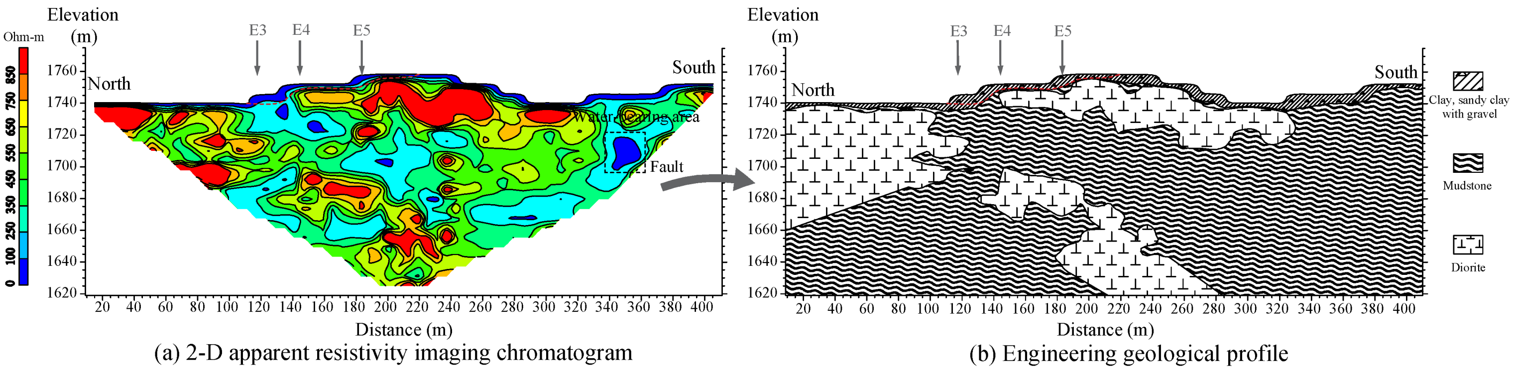
The survey line E3 is laid in the northern part of the slope, where the angle of the slope is relatively small. The low resistivity layer with a resistivity of 100 $\Omega$·m is the slope residual layer of the slope, which mainly consists of clay and sandy clay with 20~30% gravel, with a thickness of 7~10 m. As can be seen in Figure 5, the bedrock of the slope is covered by a thick layer of loosely piled soil, which is loose in structure and contains pore water. During periods of continuous heavy rainfall, the rainwater infiltrates the slope residual layer, softening the soil layer, and increasing the weight of the soil body, which may become an unstable area.

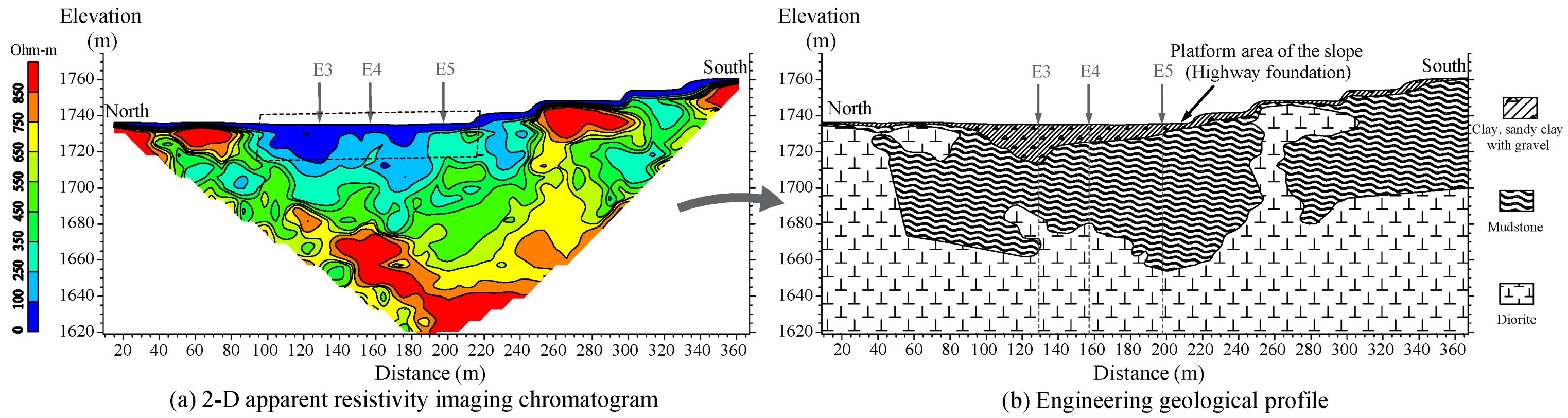
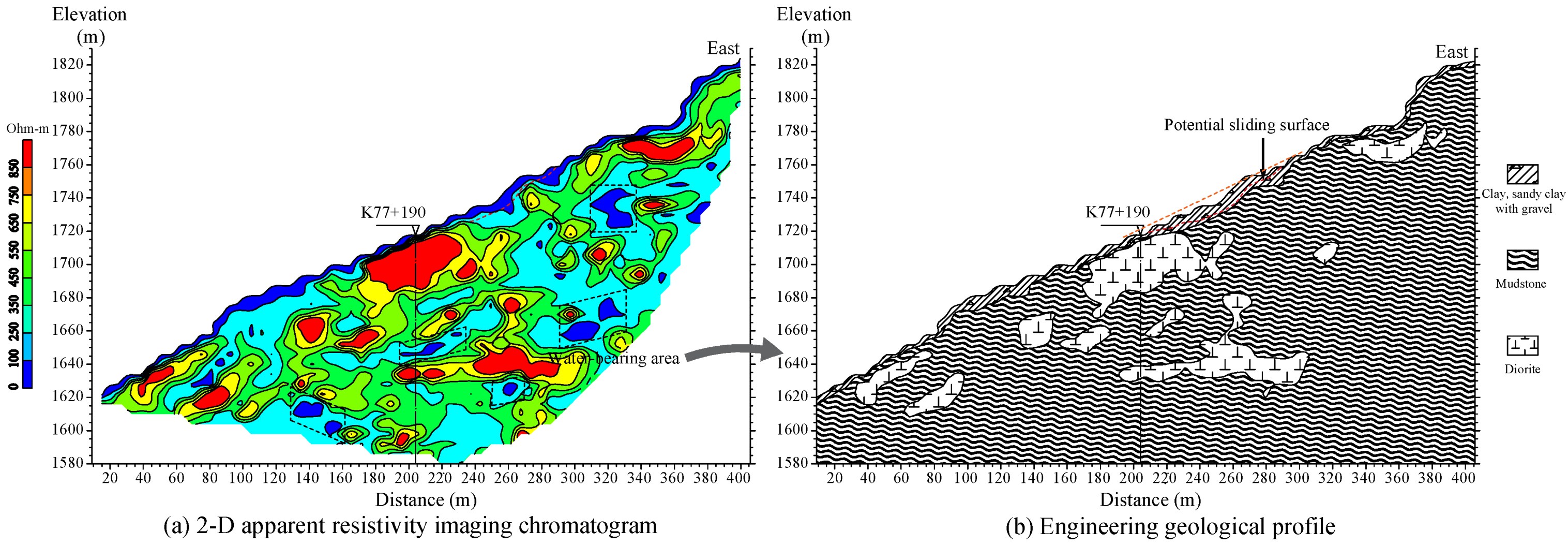
The survey line E4 is in the middle of the investigated slope, the apparent resistivity of the surface layer is low, and the residual sediment is thin, only 1~3 m. The high resistivity area in Figure 6 below the route is intrusive diorite, which is weakly weathered and has relatively high rock strength. However, the slope of the profile E4 is greater than 55°, which is a potentially unstable area. In the deep part of profile E4, there are some dark blue closed low resistivity areas, which are the reflection of the mudstone containing fissure water. The survey line E5 is on the south side of the investigated slope, the apparent resistivity of the surface layer is low, and the residual deposits are only 2~5 m. An abrupt change in apparent resistivity occurs below the route at a depth of 3 m, with a closed high-resistivity zone. The closed high resistivity zone in Figure 7 consists of weakly weathered and relatively high rock strength Diorite, which is an intrusive igneous rock. It has a high resistivity value, generally above 850 $\Omega$·m.

The above analysis shows that the topography of the studied slope is complex, similar to a ‘dustpan’ shape with varying thicknesses of overlying slope residual deposits in the lateral direction. Specifically, the thickness ranges from 0.5~1 m at the top of the slope, 2~4 m in the middle and lower slopes, and increases to 12~14 m at the foot of the slope. The apparent resistivity of the area marked by the black frame in Figure 4, Figure 6 and Figure 7 is significantly lower than that of the surrounding area, which is the reflection of the fracture water contained in the mudstone. The boundary between the low and high resistivity can be defined as the potential sliding surface of slopes, which is indicated in Figure 4, Figure 5, Figure 6 and Figure 7 by a red line. By analyzing high-density resistivity 2D inversion images and engineering geologic profiles, it is inferred that the shape of the slope sliding surface approximates a folded linear shape, and the sliding surface is roughly the contact surface that is between the slope residual deposits and the underlying strongly weathered bedrock.

3. Finite Element Stability Analysis of the Slope Based on Strength Reduction Method

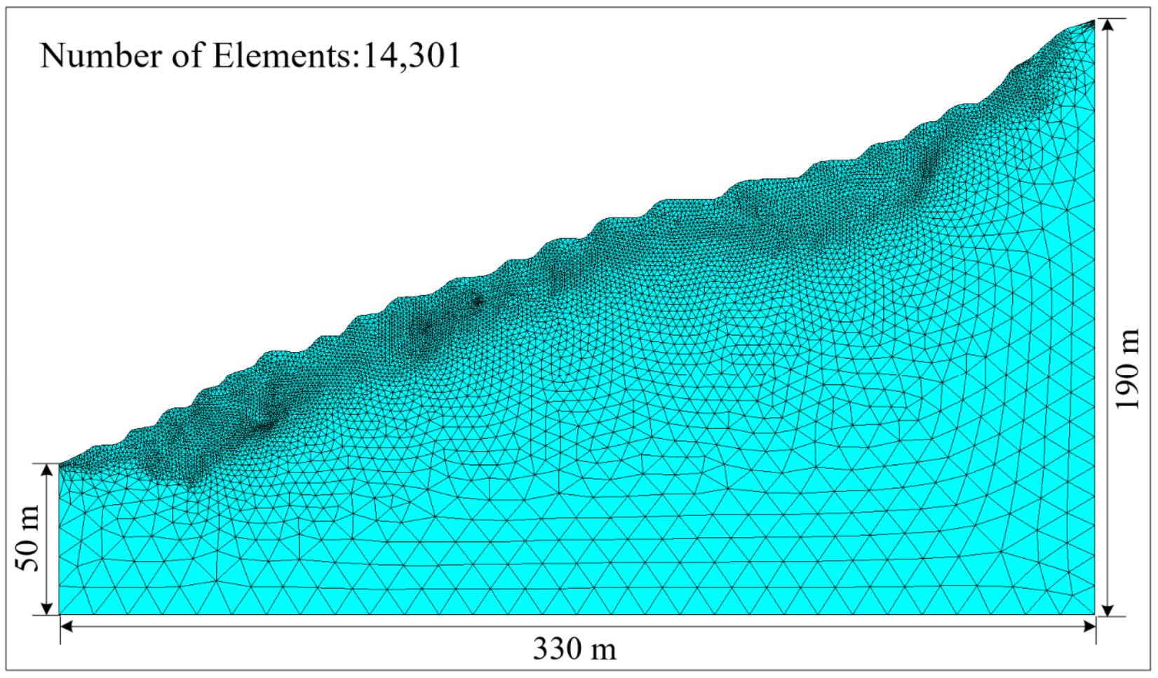
To identify specific monitoring locations and obtain effective monitoring results, a two-dimensional geometric model was established to analyze the displacement and strain characteristics of the slope using ANSYS numerical analysis software (Ansys 2021 R2). Based on slope characteristics, the simplified 2D finite element meshing model of the slope is shown in Figure 8. The stability analysis of the north profile of the slope was carried out using the strength reduction method. The basic idea of the strength reduction method is reducing the shear strength parameter of the slope geotechnical body and then bringing it into the model for calculation until the numerical calculation does not converge and the slope reaches the limit of the damage state. Ansys embedded program automatically obtains the potential slip surface of the slope based on the results of elastoplastic finite element calculations, and the safety factor of the slope is also obtained. To carry out slope stability analysis and calculation, select the initial discount factor F (generally take F = 1), and then the slope soil material strength coefficient is discounted, and the cohesion and internal friction angle after the discount with the formula are expressed as:

$$C^{\prime }={\displaystyle \frac{C}{F}}$$

(1)

$$tan{\phi }^{\prime }={\displaystyle \frac{tan\phi }{F}}$$

(2)

C and $\phi$ are the initial cohesion and the angle of internal friction of the soil body of the slope, $C^{\prime }$ and ${\phi }^{\prime }$ are the discounted cohesion and angle of internal friction, respectively. The calculation adopted displacement boundary conditions: the model was set up with horizontal and vertical fixed constraints at the bottom of the model, horizontal fixed constraints at the left and right boundaries, and no constraints at the top of the slope. According to the analysis of engineering survey data, the selected rock layer’s physical and mechanical parameters are in

Table 1. Soil and rock parameters selected in numerical analysis.

Name of the Soil	Internal Friction Angle (°)	Cohesion	Modulus of Elasticity	Poisson’s Ratio	Natural Density (KN/cm3)
Sand clay (with gravel)	20.45	13.6 Kpa	0.64 Gpa	0.32	17.9
Diorite	—	—	80 Gpa	0.25	28.5
Mudstone	36.4	0.13 Mpa	6 Gpa	0.232	26.3

.

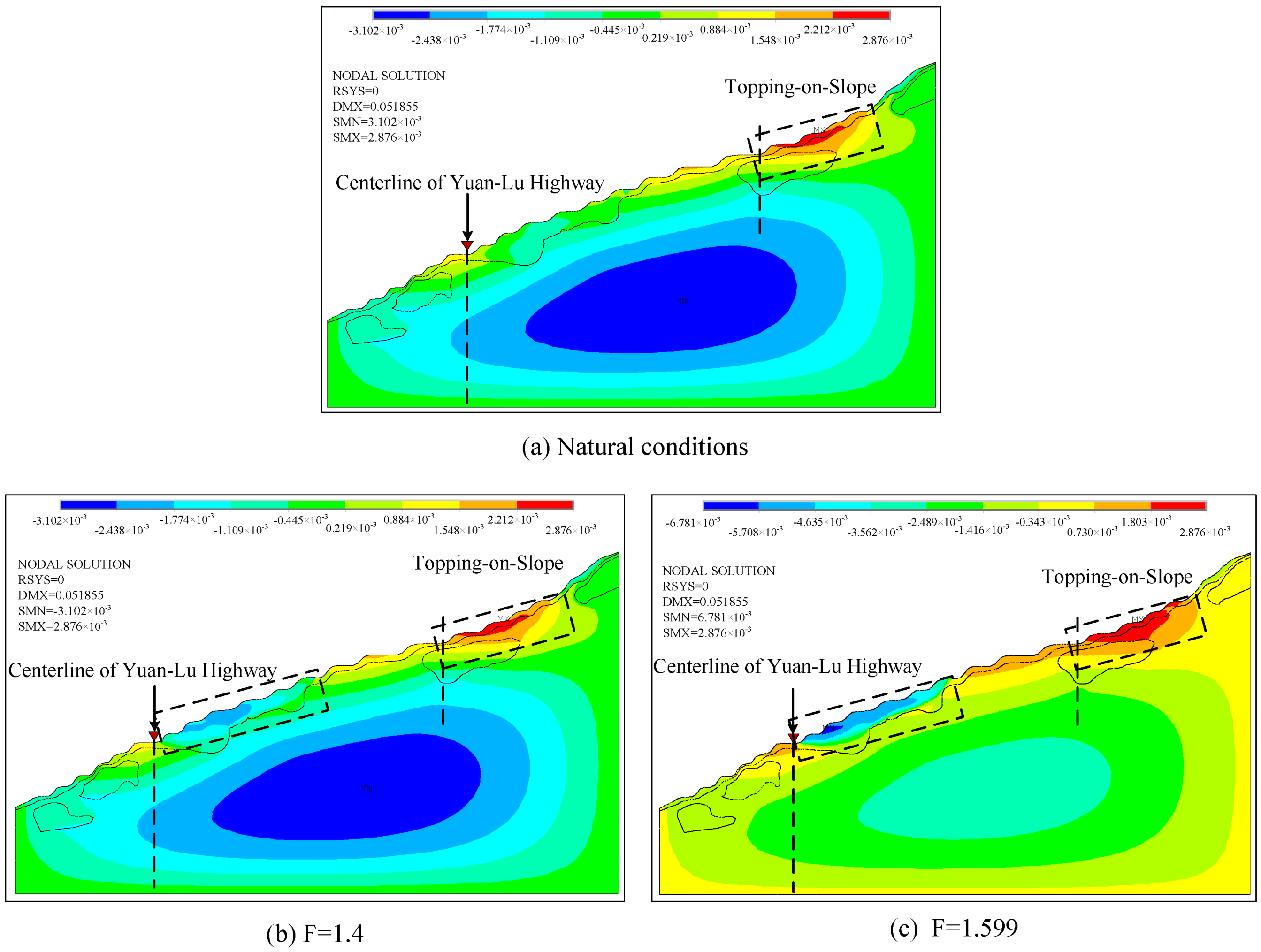
The model is divided into three zones according to the material characteristics of profile E3 from top to bottom. The upper part is the Quaternary ($Q_4^{dl+el}$) slope residual layer, the lower part is mudstone, and the middle part of the model is Diorite. Figure 9 shows the x-direction displacement diagrams of the slope profile E3 with different reduction factors. Observing Figure 9a, under the effect of natural gravity, the deformation of the slope in the horizontal direction is mainly concentrated at the top and foot of the slope. In these two areas, there is a regular layering phenomenon in the vertical direction, the displacement value gradually decreases from the surface layer to the deeper layer, and the maximum displacement of the slope occurs at the trailing edge of the slope. In addition, at the time of site investigation, tensile cracks had already appeared at the rear edge of the slope, but the width was not wide, which is consistent with the deformation trend of numerical analysis. 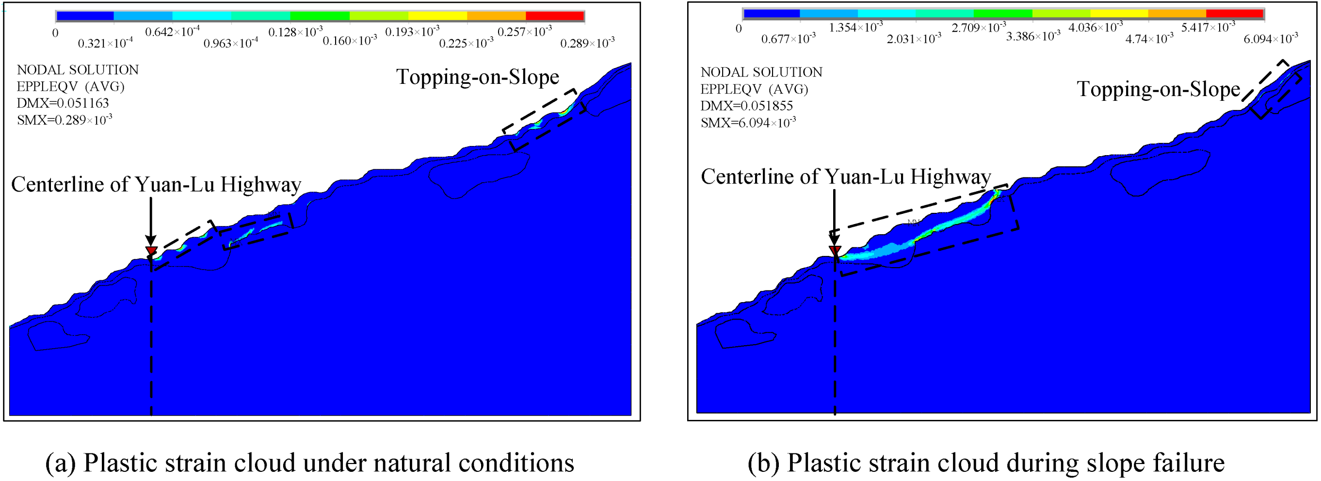Meanwhile, in the plastic strain map in Figure 10a, the plastic strain has been generated inside the slope body under natural conditions, and the plastic strain area extends from the rock interface to the upper slope residual layer but does not penetrate the slope. In addition, the numerical calculation results converge, indicating that the slope is stable under natural conditions.

As the strength reduction coefficient F increases, the plastic strain increases, and the plastic strain distribution expands. Finally, when F = 1.559, a local area of penetrating plastic strain formed in Figure 10b above the route and is roughly circular in shape. Meanwhile, the computational results of the model do not converge, which indicates that the slope is no longer safe. Through the above analysis, the deformation of the slope mainly occurs at the foot and the top of the slope, so if monitoring these two areas, the data obtained can effectively reflect the deformation trend and characteristics of the slope. However, considering that the route is situated at the foot of the slope, and the purpose of the monitoring is to obtain the deformation of the slope during the operation, the monitoring area was determined at the foot of the slope area close to the route.

The results show that the plastic deformation of the slope’s geotechnical body under self-weight is mainly concentrated at the interface between different rock bodies, distributing both up and down along the interface. In addition, according to the engineering geological structure map in Figure 5 and the plastic strain cloud in Figure 10b, it can be seen that the two speculations about the location and shape of the slope sliding surface are compatible.

Based on the team’s preliminary geologic investigation, it was determined that there are no man-made structures on the upper portion of the slope, so the building load forces on the slope are not considered. Considering that the rainy season in the slope area is mostly concentrated from May to September, and the average precipitation for many years ranges from 1450.89 to 2108.99 mm, due to the infiltration of surface water, it softens the overlying soil, which increases the heaviness of the soil, reduces the shear strength, and decreases the stability of the landslide. In this chapter, the finite element model of the slope is established to study the deformation characteristics of the slope and identify the potential slip surface using the strength reduction method. The ANSYS simulation verifies the interpretation of the high-density resistivity method for the slope sliding zone, which improves the reliability of the slope stability assessment.

4. Application and Analysis of FBG Strain Detection Piles in Slope Deformation Monitoring

According to the numerical analysis results and engineering geological conditions, in this chapter, the monitoring area is selected to be the foot of the slope near the highway, with strain detection piles to monitor the slope’s deep deformation. Array sensors implanted in concrete piles can acquire strain information at different depths as the slope deforms, thus reflecting the internal stress change characteristics of the slope. The axial force of the strain detection pile can be expressed as:

$$Q_i={\epsilon }_i·E_i·A_i$$

(3)

where $Q_i$ is the axial force at section i of the pile. ${\epsilon }_i$, $E_i$, and $A_i$ are the strain value, cross-sectional area, and modulus of elasticity at section i, respectively. The sensors used in this paper are FBG strain sensors, the reflected light wavelength of FBG varies with the change in temperature and strain, and the relationship [32] between them can be expressed as follows:

$$\frac{\Delta \lambda }{\lambda }=\left(1-P_{eff}\right)\Delta \epsilon +(\alpha +\xi )\Delta \mathrm{T}$$

(4)

where $\lambda$ is the initial Bragg wavelength, $\Delta$$\lambda$ is the variation in Bragg wavelength, $P_{eff}$ is the effective photo-elastic coefficient, $\Delta$$\epsilon$ is the applied strain, $\Delta$T is the temperature change, $\alpha$ and $\xi$ are the thermal expansion coefficient and thermal-elastic coefficient of the fiber core.

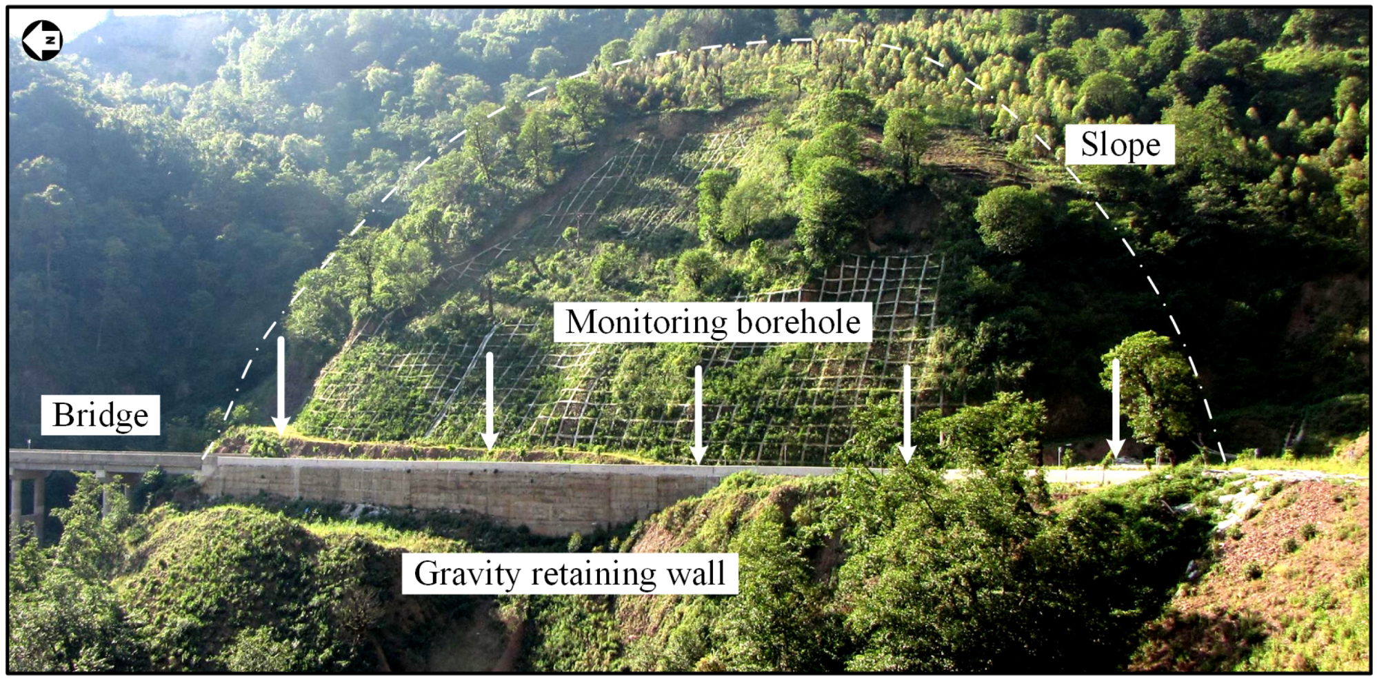
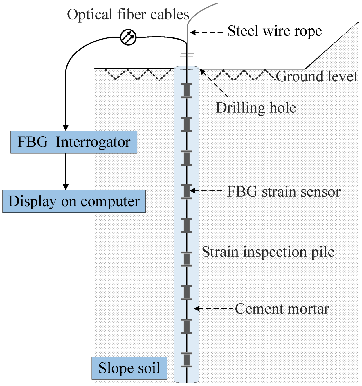
Firstly, five deformation observation boreholes (IN 1~IN 5) were arranged in turn at the foot of the slope of K77 + 120~K77 + 215 section of the secondary highway from Yuanyang to Luchun, with a depth of 30 m and a diameter of 127 mm, and the interval was about 10 m, The deployment diagram of FBG strain piles is shown in Figure 11. The FBG strain sensors are tied with wire rope and embedded in the borehole in order at 2 m intervals, and three FBG temperature sensors are installed in the upper, middle, and lower positions of the borehole for temperature compensation at different depth positions. The boreholes are then backfilled with cement mortar. After the cement mortar is consolidated, the piles for detecting slope-deep deformation are formed. The strain detection piles implanted in the slope can deform synchronously with the rock and soil mass, and the longitudinal strain change of the pile during the deep deformation is obtained through the FBG strain sensors buried in the piles, reflecting the characteristics of the slope stress changes. The working principle of FBG strain detection piles to monitor the deep deformation of the slope is shown in Figure 12.

In practical applications, FBG strain sensors with different central wavelength values were used because the same wavelength will cause the signals received by the demodulator to overlap, and the specific position of the sensor cannot be identified from the wavelength value received by the demodulator. The wavelength interval of the FBG sensor used for slope monitoring in this paper is more than 3 nm. The fiber Bragg grating strain sensor had a strain monitoring error of less than 10 µ$\epsilon$, a measurement range of −1000 to 1000 µ$\epsilon$, and a resolution of 0.7 µ$\epsilon$. 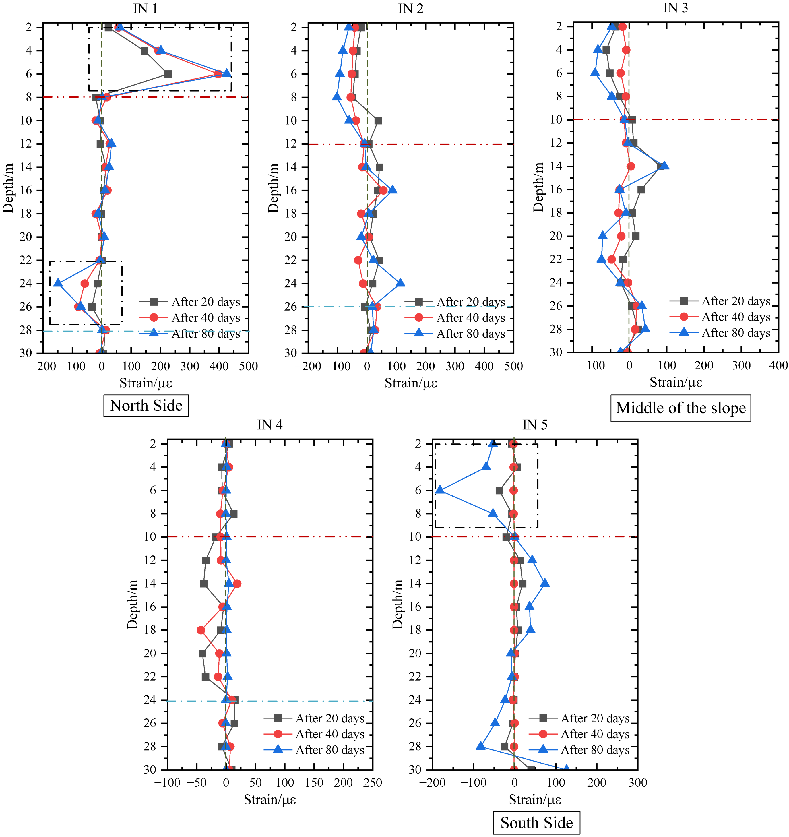The FBG monitoring system was completed on 27 January 2014, and initial strain data were collected on 22 February 2014. Then, the strain monitoring data were collected after 20 days (14 March), 40 days (3 April), and 80 days (13 May). The variation in the longitudinal strain of the detection pile IN 1~IN 5 is shown in Figure 13. Positive strain indicates that the strain sensor is under tension; a negative strain indicates that the strain sensor is under compression.

FBG field monitoring mainly focuses on the deep deformation of the slope. According to the deformation data of IN 1~IN 5, it was found that the strain variation in the shallow surface on the north side of the slope is large, especially at a depth of 6 m of IN 1; the maximum strain value obtained by the FBG sensors is 426 µ$\epsilon$, and the maximum strain change value obtained at 4 m is nearly 200 µ$\epsilon$, which is much larger than the other positions, so it can be assumed that shear deformation occurs at a depth of 6 m on the north side of the slope. Corresponding to the strongly weathered fractured structural surface between the residual slope deposit of clay and the underlying mudstone, the strain value at a depth of 8~22 m is very small, so it is assumed that the positions in this depth range are located in a weakly weathered and stable zone of bedrock. The strain value increases at a depth of 22 m to 28 m, with the maximum value reaching 149 µ$\epsilon$, which suggests that there may be fissure water inside the soil body at this place. When rainfall occurs, the infiltration of rainfall will cause changes in the water content of the slope, resulting in the corresponding adjustment of the stress field and displacement field in the soil. During the period from 2 April to 5 April, continuous rainfall occurred in the monitoring area. Infiltration of rainwater into the ground increases the soil saturation, which is inimical to slope stability. Because the overlying slope residue on the north side of the slope is thicker, ground movement due to significant rainfall infiltration also leads to obvious lateral strain change of IN1 in the shallow areas. The average strain values at IN 2~IN 4 were relatively small in changes, and the structure is comparatively stable. The strain variation in the shallow surface on the south side of the slope is large, especially at a depth of 6 m of IN 5, corresponding to the depth of the rock boundary location.

The average strain values at IN 2~IN 4 were relatively small in changes, and the structure is comparatively stable. The strain variation in the shallow surface on the south side of the slope is large, especially at a depth of 6 m of IN 5, corresponding to the depth of the rock boundary location. In addition, the longitudinal strain distribution characteristics indicated that the cumulative deformation of the shallow soil on the northernmost and southernmost sides of the slope is significantly larger than that of the deep soil. Moreover, there is a zone of stability with a small variation in the strain at the bottom of boreholes IN 1, IN 2, and IN 4. The presence of these stable zones suggests that the bottom of the borehole is positioned in a zone of stability within the bedrock. In summary, the utilization of FBG strain sensors to grasp the stress–strain law of the slope provides an effective monitoring method for slope stability evaluation.

5. Discussion and Conclusions

The determination of the location, distribution, direction, and depth of the potential slip zone on the slope is the key to the slope condition assessment. In this paper, the high-density resistivity method, numerical simulation, and FBG deformation monitoring technology are combined to provide a reliable method for slope stability evaluation. The main conclusions of this study can be summarized as follows:

(1) According to the geological environment of the slope, the corresponding high-density resistivity survey line layout scheme is proposed. Based on the conversion and analysis of the detection results, the engineering geological structure map of the slope is obtained, and the potential slip surface is delimited preliminarily.

(2) The comprehensive analysis shows that the slope residual layer on the north side of the slope is thick, which makes it easy to slide under the influence of external factors. On this basis, the section of the north side of the slope is extracted and analyzed.

(3) The 2D finite element analysis model of the slope is established by ANSYS. The position and shape of the potential sliding surface are determined by the simulation results, which are consistent with the results of the high-density resistivity method.

(4) The FBG monitoring system is set up in the selected monitoring area, and the deformation and change trend of the slope are understood by analyzing the longitudinal strain monitoring data of the sensor.

(5) During the monitoring period, the longitudinal strain of IN 2~IN 4 fluctuated in a small amplitude, and the strain in the shallow area of IN 1 and IN 5 varied more, with the maximum values reaching 426 µ$\epsilon$ and −182 µ$\epsilon$, respectively. The monitoring and analysis of these two areas should be strengthened in later stages.

Based on this paper, further research can be carried out. For example, the cross-section and longitudinal section of the slope can be combined to establish a three-dimensional model of the slope for stability analysis. However, this needs to be supported by more detailed geological data on the slope.