Evaluation of Interval Type-2 Fuzzy Neural Super-Twisting Control Applied to Single-Phase Active Power Filters

Abstract

This research introduces an improved control strategy for an active power filter (APF) system. It utilizes an adaptive super-twisting sliding mode control (STSMC) scheme. The proposed approach integrates an interval type-2 fuzzy neural network with a self-feedback recursive structure (IT2FNN-SFR) to enhance the overall performance of the APF system. The IT2FNN with STSMC proposed here consists of two components, with one being IT2FNN-SFR, which demonstrates robustness for uncertain systems and the ability to utilize historical information. The IT2FNN-SFR estimator is used to approximate the unknown nonlinear function within the APF. Simultaneously, the STSMC component is integrated to reduce system chattering, improving control precision and overall system performance. STSMC combines the robustness and simplicity of traditional sliding mode control, effectively addressing the chattering problem. To mitigate inaccuracies and complexities associated with manual parameter setting, an adaptive law of sliding mode gain is formulated to achieve optimal gain solutions. This adaptive law is designed within the STSMC framework, facilitating parameter optimization. Experimental validation is conducted to verify the harmonic suppression capability of the control strategy. The THD corresponding to the designed control algorithm is 4.16%, which is improved by 1.24% and 0.55% compared to ASMC and STSMC, respectively, which is below the international standard requirement of 5%. Similarly, the designed controller also demonstrates advantages in dynamic performance: when the load decreases, it is 4.72%, outperforming ASMC and STSMC by 1.15% and 0.38%, respectively; when the load increases, it is 3.87%, surpassing ASMC and STSMC by 1.07% and 0.36%, respectively.

1. Introduction

With increasing types of loads, especially due to the introduction of power electronic equipment, undesirable harmonic components are injected into the power grid, which pose a serious threat to power quality and equipment life [1]. Active power filters have been verified as the most widely used solution to address these issues, which can generate counteractive currents or voltages to compensate for adverse harmonic components in power systems, thereby enhancing power quality [2,3]. Excellent control algorithms can give full play to the advantages of APF’s fast response and excellent compensation performance.

In contemporary applications, sliding mode control (SMC) is extensively employed to address diverse nonlinear challenges owing to its rapid dynamic response, stability, and robustness to external disturbances [4,5,6,7]. However, the most characteristic feature of SMC is the discontinuous control, which will result in unexpected chattering when approaching the sliding mode surface. Introducing fractional-order theory into sliding mode control can better describe some nonlinear dynamic characteristics, improve control performance and robustness, and effectively reduce chattering issues [8,9,10]. However, fractional-order sliding mode control involves fractional-order calculus, leading to increased complexity in mathematical models and algorithms, which in turn increases the difficulty of computation and implementation. Additionally, parameter tuning for fractional-order sliding mode control is relatively challenging. Super-twisting sliding mode control is also commonly used to suppress chattering in controllers, which generates continuous control signals, effectively reducing chattering [11,12,13]. A new composite controller integrating STSMC was devised for speed and altitude tracking control in air-breathing hypersonic vehicles [14]. This illustrates the versatility and applicability of STSMC in addressing chattering-related challenges across various control domains.

The great approximation performance of neural networks has been verified in many studies [15,16,17]. In [18], Sun et al. incorporated an RBF neural network into a primary controller, achieving the faster and more accurate recovery of unknown disturbances, thereby addressing the issue of system uncertainty. Fuzzy logic rules are considered as one of the effective approaches to deal with nonlinear problems. Incorporating fuzzy rules into neural networks proves highly advantageous for enhancing their performance [19,20,21,22]. The implementation of an adaptive universal type-2 fuzzy neural network control system enhances the anti-interference capability in the motion balance of power line inspection robots [23]. For neural networks designed for dynamic pattern recognition, the introduction of a self-feedback structure enables the storage and utilization of historical information, thereby enhancing the network’s memory capacity and better adapting to changes and uncertainties [24,25,26,27]. While the theoretical validation of the method has been conducted in previous studies, the feasibility and superiority of the algorithm in simulations are primary concerns. Hence, the simulation environment is an ideal experimental setting, allowing for the selection of high sampling frequencies to achieve rapid data acquisition [28]. However, in practical applications, constraints on the computational capabilities of control devices often prevent the realization of the ideal sampling frequencies observed in simulations. Therefore, the designed method needs to be validated for its feasibility on a hardware experimental platform. Inspired by the preceding studies, this paper proposes an adaptive super-twisting sliding mode control method, incorporating an interval type-2 fuzzy neural network with a self-feedback recursive structure (IT2FNN-SFR STSMC), aiming to enhance the compensation accuracy of the APF system. The novel IT2FNN-SFR consolidates the advantages of IT2FNN and RNN, leading to superior dynamic approximation capacity.

The primary contributions of this article are outlined as follows: (1) A novel structure named IT2FNN-SFR has been presented, which amalgamates the robustness inherent in IT2FNN with the dynamic response characteristics of Recurrent Neural Networks (RNNs). This newly introduced neural network operates in an error-driven and online-optimized manner, reducing its dependence on precise system information. The recursive structure within the neural network enables the storage and utilization of historical information, thereby enhancing estimation accuracy and dynamic approximation. (2) STSMC merges the robustness and simplicity inherent in traditional sliding mode control, effectively mitigating the chattering phenomenon. To mitigate inaccuracies and complexities stemming from manual parameter adjustment, a sliding mode gain adaptive law was devised to attain an optimal array of gain solutions. (3) The designed controller algorithm was tested on the corresponding hardware experimental platform and had better harmonic compensation performance than the traditional ASMC and STSMC, verifying its feasibility under actual working conditions.

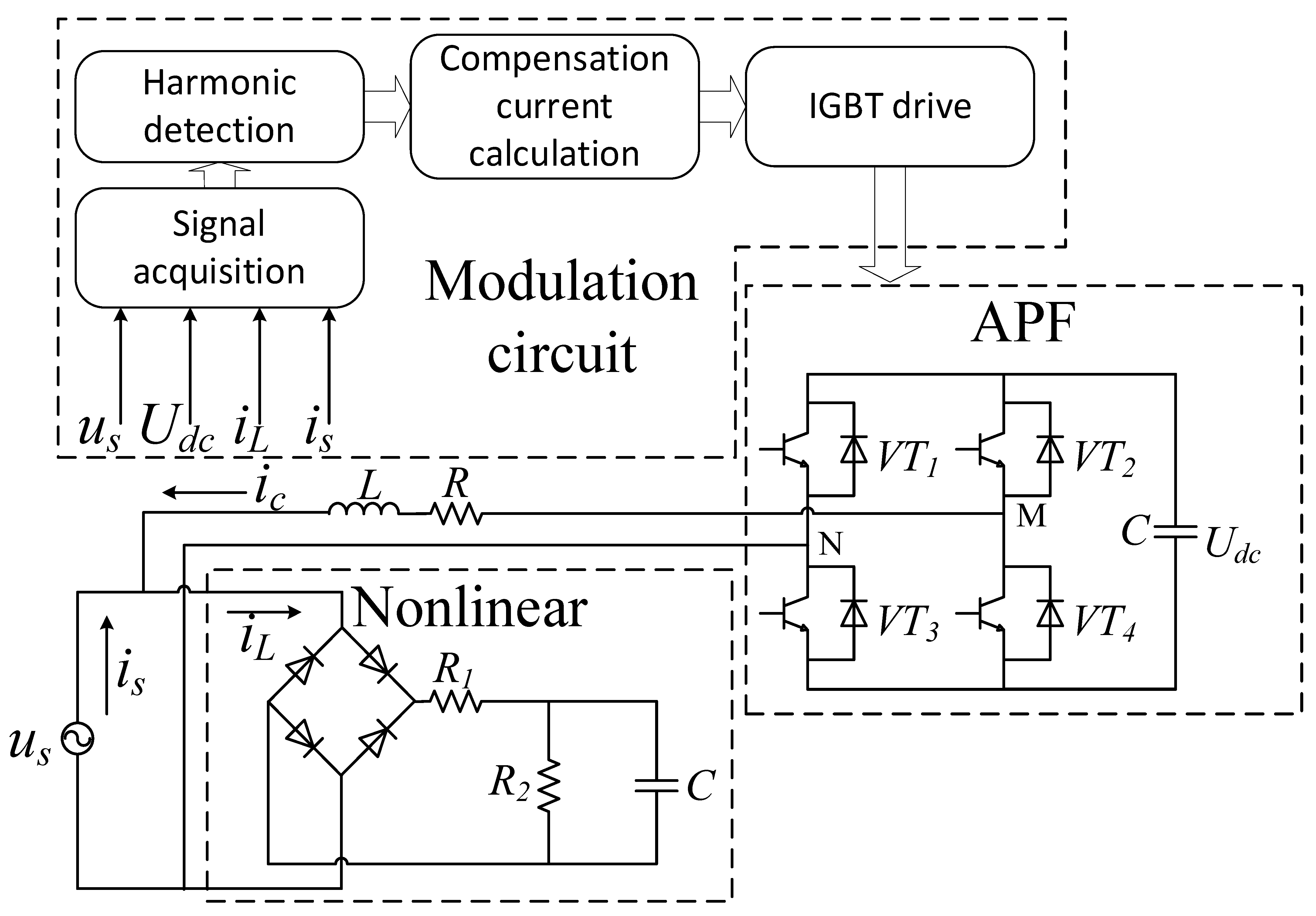
2. Mathematical Model of Active Power Filter

Figure 1 illustrates the fundamental circuit configuration of single-phase active power filter (APF) system control. The working principle of the APF is as follows: The APF collects current signal $i_s$, voltage signal $u_s$, DC-side voltage signal $U_{dc}$, and load current signal $i_L$ through sensors, extracting the harmonic signals from them. The controller generates corresponding control signals based on the extracted harmonic signals. These signals are modulated through PWM and control the conduction and turn-off of power semiconductor devices (IGBTs are used as an example in this paper) via a driving circuit, thereby generating compensating current $i_c$ to counteract the adverse components in the original grid current. In addition, the equivalent inductance and resistance of the APF circuit are $L$ and $R$.

With reference to [15], the practical system can be simplified as follows:

$$\dot{x}=f+bu$$

(1)

where $f=f(x)+g(t)=-\frac{R}{L}{i}_c-\frac{u_s}{L}-\frac{U_{dc}}{L}+g(t)$, and $g(t)$ represents the overall disturbance, encompassing both parameter perturbation and external disturbance.

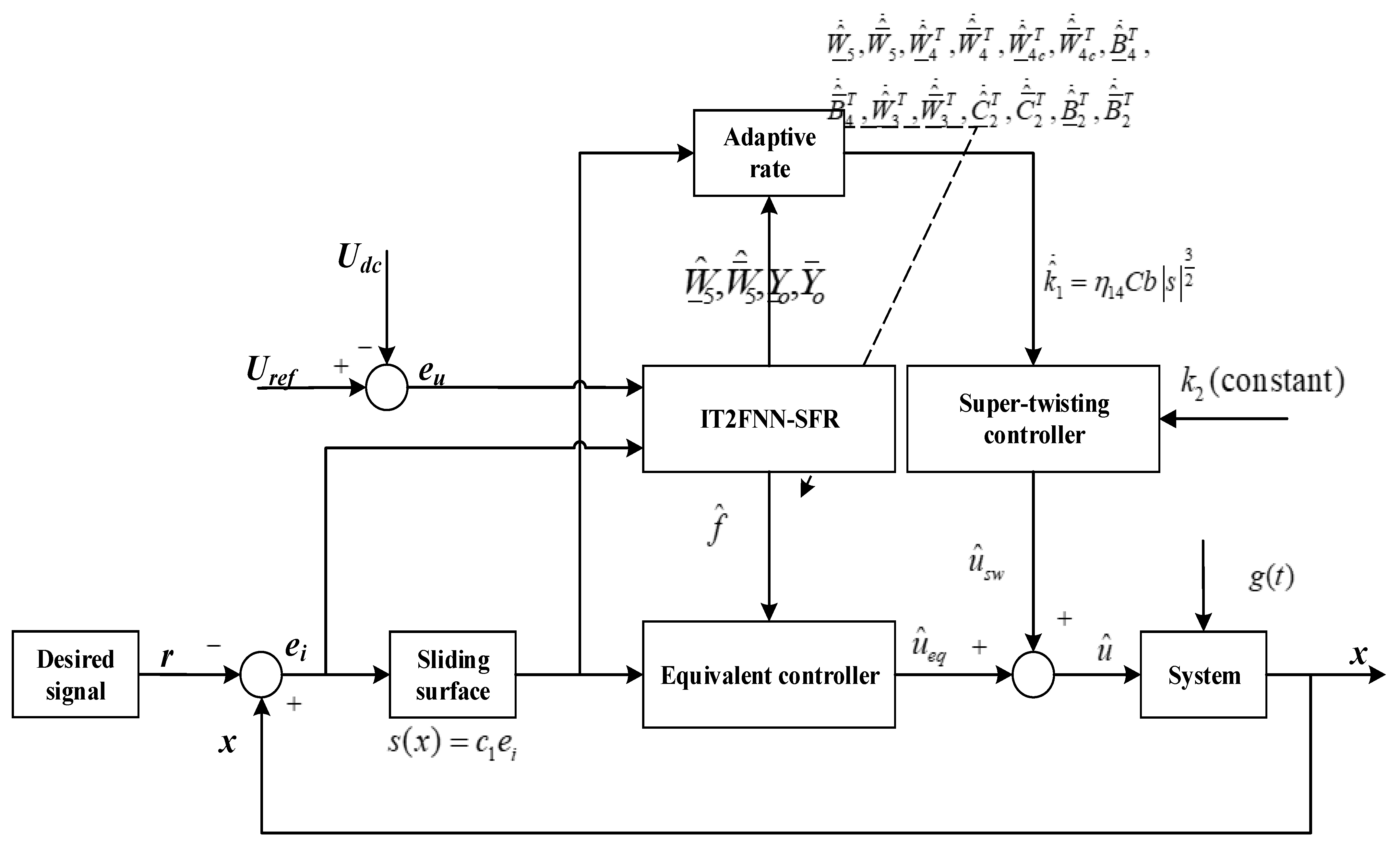
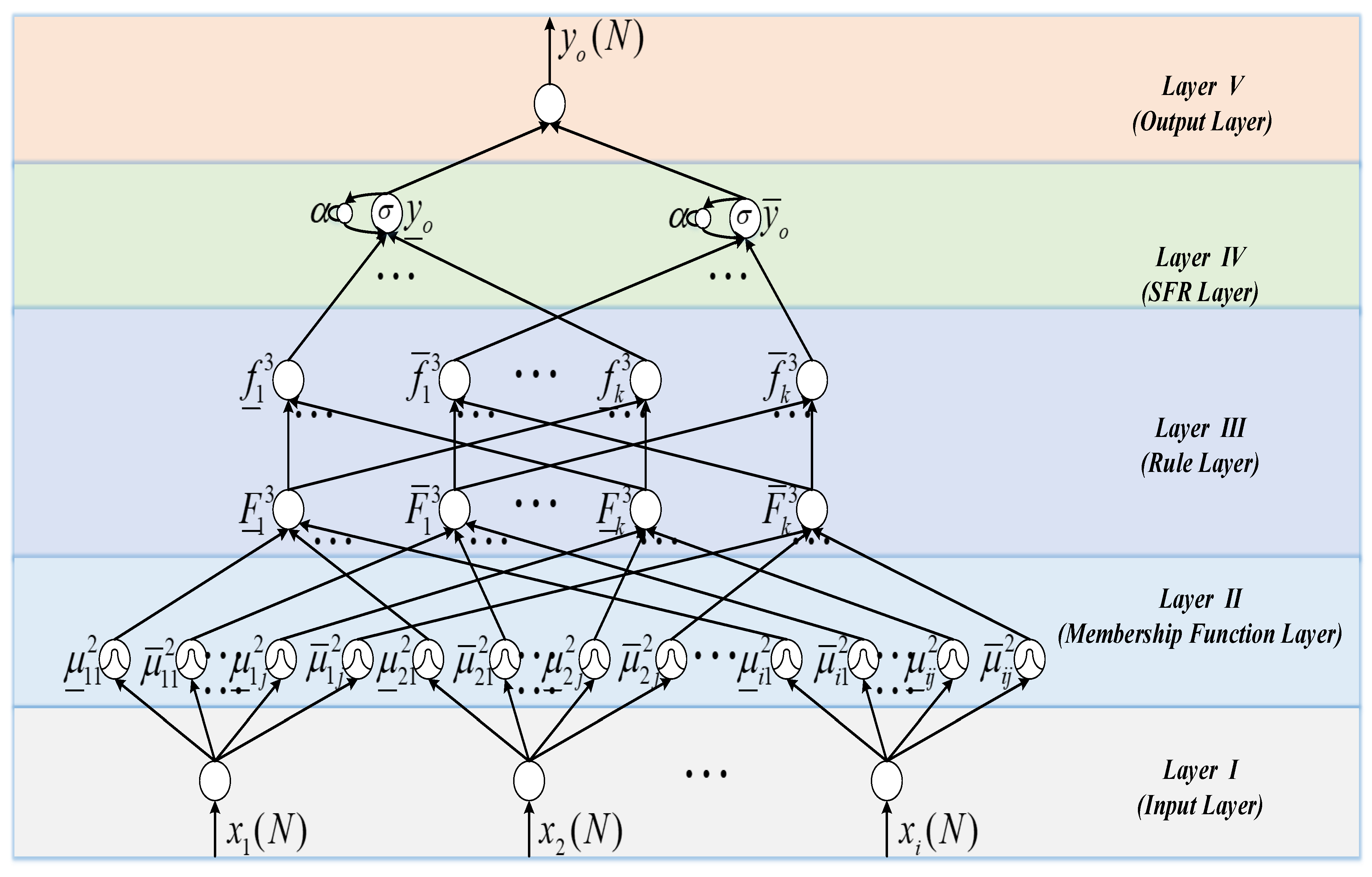
3. Controller Design and Analysis

The comprehensive control strategy is outlined in the framework diagram presented in Figure 2. The architecture of the innovative networks is illustrated in Figure 3.

Layer I (input layer): The input of the neural network is customized according to the requirements of the specific problem and introduced into the network processing through this layer. The signal transfer of this layer is expressed as follows:

$$ne{t}_i^1(N)=x_i^1(N)$$

(2)

$$y_i^1\left(N\right)=f_i^1\left(ne{t}_i^1(N)\right)=ne{t}_i^1(N)$$

(3)

where $x_i^1(N)$ and $y_i^1(N)$ represent the input and output of the node, respectively, the superscript represents the number of layers in which the variable exists, the subscript represents the input number corresponding to the variable, and N represents the number of sampling cycles.

Layer II (membership function layer/fuzzy layer): In this layer, Gaussian functions with center vectors and uncertain base widths are utilized to enhance the neural network’s capability in handling nonlinearity. Let the j-th group in the type-2 fuzzy output set be defined as $[{\underset{\_}{\mu }}_{ij}^2,{\overline{\mu }}_{ij}^2]$. The relationship between input and output is expressed as follows:

$$x_{ij}^2(N)=y_i^1(N)$$

(4)

$${\underset{\_}{\mu }}_{ij}^2(N)=\exp \left[-\frac{1}{2}{\left(\frac{x_{ij}^2(N)-{\underset{\_}{c}}_{ij}^2}{{\underset{\_}{\sigma }}_{ij}^2}\right)}^2\right]$$

(5)

$${\overline{\mu }}_{ij}^2(N)=\exp \left[-\frac{1}{2}{\left(\frac{x_{ij}^2(N)-{\overline{c}}_{ij}^2}{{\overline{\sigma }}_{ij}^2}\right)}^2\right]$$

(6)

where ${\mu }_{ij}^2$, $c_{ij}^2$, and ${\sigma }_{ij}^2$ represent the output of the node, the center vector, and the base width of the Gaussian function, respectively. In addition, the lower bound and upper bound of the variable are distinguished by “$\underset{\_}{\ast }$” and “$\overline{\ast }$”, respectively.

Layer III (rule layer): This layer consolidates input signals received from the preceding layer. The detailed rules are expressed as follows:

$${\underset{\_}{F}}_k^3={\displaystyle \prod _{i=1}^I{\underset{\_}{\mu }}_{ij}^2};{\overline{F}}_k^3={\displaystyle \prod _{i=1}^I{\overline{\mu }}_{ij}^2}$$

(7)

$${\underset{\_}{f}}_k^3=\frac{{\underset{\_}{F}}_k^3}{{\displaystyle \sum _{k=1}^K{\underset{\_}{F}}_k^3}};{\overline{f}}_k^3=\frac{{\overline{F}}_k^3}{{\displaystyle \sum _{k=1}^K{\overline{F}}_k^3}}$$

(8)

where $f_k^3$ represents the output of the rule layer after normalization.

Layer IV (self-feedback recursive layer): This layer integrates signals from the rule layer with past information regarding this layer’s output (handled and stored through a temporary recursive structure), and the specific operational logic is as follows:

$${\underset{\_}{x}}^4(N)={\displaystyle \sum {\underset{\_}{\omega }}_k^3{\underset{\_}{f}}_k^3}$$

(9)

$${\underset{\_}{x}}^{4c}(N)=\alpha {\underset{\_}{x}}^{4c}(N-1)+{\underset{\_}{y}}^4(N-1)$$

(10)

$$n\underset{\_}{e}{t}^4(N)={\underset{\_}{\omega }}^4{\underset{\_}{x}}^4(N)+{\underset{\_}{\omega }}^{4c}{\underset{\_}{x}}^{4c}(N)+{\underset{\_}{b}}^4$$

(11)

$${\underset{\_}{y}}^4(N)=\sigma \left(n\underset{\_}{e}{t}^4(N)\right)$$

(12)

$${\overline{x}}^4(N)={\displaystyle \sum {\overline{\omega }}_k^3{\overline{f}}_k^3}$$

(13)

$${\overline{x}}^{4c}(N)=\alpha {\overline{x}}^{4c}(N-1)+{\overline{y}}^4(N-1)$$

(14)

$$n\overline{e}{t}^4(N)={\overline{\omega }}^4{\overline{x}}^4(N)+{\overline{\omega }}^{4c}{\overline{x}}^{4c}(N)+{\overline{b}}^4$$

(15)

$${\overline{y}}^4(N)=\sigma \left(n\overline{e}{t}^4(N)\right)$$

(16)

$$\sigma (z)=\frac{1}{1+e^{-z}}$$

(17)

where $x^4(N)$ denotes the signal from the rule layer at the current sampling time; $x^{4c}(N)$ represents the historical information stored in the temporary recursive structure; ${\omega }^{4c}$ represents a self-feedback weight; ${\omega }^4$ signifies the weight of the SFR layer; $\alpha$ serves as the self-feedback gain, determining the weighting of historical information; $b_l^4$ is a bias term; $\sigma (\cdot )$ denotes a sigmoid activation function.

Layer V (output layer): The output of the network is computed through weighted operation, expressed as follows:

$$y_o(N)={\underset{\_}{\omega }}^5{\underset{\_}{y}}^4(N)+{\overline{\omega }}^5{\overline{y}}^4(N)$$

(18)

The super-twisting sliding mode control (STSMC) is implemented to mitigate chattering. In this study, an adaptive rate for gain $k_1$ is additionally devised to alleviate the challenges associated with parameter adjustment, as illustrated in Figure 2. Assume the tracking error of the APF system is as follows:

$$e=x-x_r$$

(19)

where $x$ corresponds to the actual compensation current in the APF system and $x_r$ represents its expected value.

The sliding mode surface is defined as follows:

$$s=Ce$$

(20)

where $C$ serves as the sliding mode surface gain, which is a positive constant.

Integrated with the neural network output $\widehat{f}$, the control strategy is formulated as follows:

$$u=\frac{1}{b}(-\widehat{f}+\dot{r})-{\widehat{k}}_1{\left|s\right|}^{\frac{1}{2}}\mathrm{sgn}(s)-{\displaystyle \int k_2\mathrm{sgn}(s)dt}$$

(21)

where $k_1>0$ and $k_2>0$.

According to the properties of the neural network, the following results can be deduced:

$$f={{\underset{\_}{W}}_5^{*}}^T{\mathsf{\Phi }}^{*}({\underset{\_}{W}}_4^{*},{\underset{\_}{W}}_{4c}^{*},{\underset{\_}{B}}_4^{\ast },{\underset{\_}{W}}_3^{*},{\underset{\_}{B}}_2^{*},{\underset{\_}{C}}_2^{*})+{{\overline{W}}_5^{*}}^T{\mathsf{\Phi }}^{*}({\overline{W}}_4^{*},{\overline{W}}_{4c}^{*},{\overline{B}}_4^{\ast },{\overline{W}}_3^{*},{\overline{B}}_2^{*},{\overline{C}}_2^{*})+\epsilon$$

(22)

where $\epsilon$ represents the difference between the desired and actual values and ${\underset{\_}{C}}_2^{*}$, ${\overline{C}}_2^{*}$, ${\underset{\_}{B}}_2^{*}$, ${\overline{B}}_2^{*}$, ${\underset{\_}{W}}_3^{*}$, ${\overline{W}}_3^{*}$, ${\underset{\_}{W}}_4^{*}$, ${\overline{W}}_4^{*}$, ${\underset{\_}{W}}_{4c}^{*}$, ${\overline{W}}_{4c}^{*}$, ${\underset{\_}{W}}_5^{*}$, ${\overline{W}}_5^{*}$, ${\underset{\_}{B}}_4^{\ast }$, and ${\overline{B}}_4^{\ast }$ denote the optimal parameters.

For further simplicity of presentation, the following is defined:

$$\underset{\_}{\mathsf{\Phi }}=\mathsf{\Phi }({\underset{\_}{W}}_4,{\underset{\_}{W}}_{4c},{\underset{\_}{B}}_4,{\underset{\_}{W}}_3,{\underset{\_}{B}}_2,{\underset{\_}{C}}_2)$$

(23)

$$\overline{\mathsf{\Phi }}=\mathsf{\Phi }({\overline{W}}_4,{\overline{W}}_{4c},{\overline{B}}_4,{\overline{W}}_3,{\overline{B}}_2,{\overline{C}}_2)$$

(24)

The output of IT2FNN-SFR is utilized as a substitute for $f$, denoted as follows:

$$\widehat{f}=y_o={{\widehat{\underset{\_}{W}}}_5}^T\widehat{\underset{\_}{\mathsf{\Phi }}}+{{\widehat{\overline{W}}}_5}^T\widehat{\overline{\mathsf{\Phi }}}$$

(25)

where the superscript “$^$” of the variables indicates their estimated value.

The approximation error of the designed neural network is represented by the following:

$$\begin{array}{l}\tilde{f}=f-\widehat{f}={{\underset{\_}{W}}_5^{*}}^T{\underset{\_}{\mathsf{\Phi }}}^{*}+{{\overline{W}}_5^{*}}^T{\overline{\mathsf{\Phi }}}^{*}+\epsilon -({{\widehat{\underset{\_}{W}}}_5}^T\widehat{\underset{\_}{\mathsf{\Phi }}}+{{\widehat{\overline{W}}}_5}^T\widehat{\overline{\mathsf{\Phi }}})\\ ={{\widehat{\underset{\_}{W}}}_5}^T\widetilde{\underset{\_}{\mathsf{\Phi }}}+{{\widetilde{\underset{\_}{W}}}_5}^T\widehat{\underset{\_}{\mathsf{\Phi }}}+{{\widehat{\overline{W}}}_5}^T\widetilde{\overline{\mathsf{\Phi }}}+{{\tilde{\overline{W}}}_5}^T\widehat{\overline{\mathsf{\Phi }}}+{\epsilon }_0\end{array}$$

(26)

where the superscript “$˜$” represents the estimation error; ${\epsilon }_0={{\widetilde{\underset{\_}{W}}}_5}^T\widetilde{\underset{\_}{\mathsf{\Phi }}}+{{\tilde{\overline{W}}}_5}^T\widetilde{\overline{\mathsf{\Phi }}}+\epsilon$ denotes the total integration of approximation errors.

Expanding Taylor series for both ${\underset{\_}{\mathsf{\Phi }}}^{*}$ and ${\overline{\mathsf{\Phi }}}^{*}$, the subsequent results can be derived as follows:

$$\underset{\_}{\tilde{\mathsf{\Phi }}}={\underset{\_}{\mathsf{\Phi }}}_{{\underset{\_}{W}}_4}{\widetilde{\underset{\_}{W}}}_4+{\underset{\_}{\mathsf{\Phi }}}_{{\underset{\_}{W}}_{4c}}{\widetilde{\underset{\_}{W}}}_{4c}+{\underset{\_}{\mathsf{\Phi }}}_{{\underset{\_}{B}}_4}{\widetilde{\underset{\_}{B}}}_4+{\underset{\_}{\mathsf{\Phi }}}_{{\underset{\_}{W}}_3}{\widetilde{\underset{\_}{W}}}_3+{\underset{\_}{\mathsf{\Phi }}}_{{\underset{\_}{C}}_2}{\widetilde{\underset{\_}{C}}}_2+{\underset{\_}{\mathsf{\Phi }}}_{{\underset{\_}{B}}_2}{\widetilde{\underset{\_}{B}}}_2+{\underset{\_}{O}}_h$$

(27)

$$\widetilde{\overline{\mathsf{\Phi }}}={\overline{\mathsf{\Phi }}}_{{\overline{W}}_4}{\tilde{\overline{W}}}_4+{\overline{\mathsf{\Phi }}}_{{\overline{W}}_{4c}}{\tilde{\overline{W}}}_{4c}+{\overline{\mathsf{\Phi }}}_{{\overline{B}}_4}{\tilde{\overline{B}}}_4+{\overline{\mathsf{\Phi }}}_{{\overline{W}}_3}{\tilde{\overline{W}}}_3+{\overline{\mathsf{\Phi }}}_{{\overline{C}}_2}{\tilde{\overline{C}}}_2+{\overline{\mathsf{\Phi }}}_{{\overline{B}}_2}{\tilde{\overline{B}}}_2+{\overline{O}}_h$$

(28)

where ${\underset{\_}{O}}_h$ and ${\overline{O}}_h$ represent extended high-order terms, and the above partial derivatives satisfy the Jacobian matrix arrangement.

By substituting (27) and (28) into (26), the following can be obtained:

$$\begin{array}{l}\tilde{f}={{\widehat{\underset{\_}{W}}}_5}^T{\underset{\_}{\mathsf{\Phi }}}_{{\underset{\_}{W}}_4}{\widetilde{\underset{\_}{W}}}_4+{{\widehat{\underset{\_}{W}}}_5}^T{\underset{\_}{\mathsf{\Phi }}}_{{\underset{\_}{W}}_{4c}}{\widetilde{\underset{\_}{W}}}_{4c}+{{\widehat{\underset{\_}{W}}}^T}_5{\underset{\_}{\mathsf{\Phi }}}_{{\underset{\_}{B}}_4}{\widetilde{\underset{\_}{B}}}_4+{{\widehat{\underset{\_}{W}}}_5}^T{\underset{\_}{\mathsf{\Phi }}}_{{\underset{\_}{W}}_3}{\widetilde{\underset{\_}{W}}}_3+{{\widehat{\underset{\_}{W}}}_5}^T{\underset{\_}{\mathsf{\Phi }}}_{{\underset{\_}{C}}_2}{\widetilde{\underset{\_}{C}}}_2+{{\widehat{\underset{\_}{W}}}_5}^T{\underset{\_}{\mathsf{\Phi }}}_{{\underset{\_}{B}}_2}{\widetilde{\underset{\_}{B}}}_2+{{\widetilde{\underset{\_}{W}}}_5}^T\widehat{\underset{\_}{\mathsf{\Phi }}}\\ +{{\widehat{\overline{W}}}_5}^T{\overline{\mathsf{\Phi }}}_{{\overline{W}}_4}{\tilde{\overline{W}}}_4+{{\widehat{\overline{W}}}_5}^T{\overline{\mathsf{\Phi }}}_{{\overline{W}}_{4c}}{\tilde{\overline{W}}}_{4c}+{{\widehat{\overline{W}}}_5}^T{\overline{\mathsf{\Phi }}}_{{\overline{B}}_4}{\tilde{\overline{B}}}_4+{{\widehat{\overline{W}}}_5}^T{\overline{\mathsf{\Phi }}}_{{\overline{W}}_3}{\tilde{\overline{W}}}_3+{{\widehat{\overline{W}}}_5}^T{\overline{\mathsf{\Phi }}}_{{\overline{C}}_2}{\tilde{\overline{C}}}_2+{{\widehat{\overline{W}}}_5}^T{\overline{\mathsf{\Phi }}}_{{\overline{B}}_2}{\tilde{\overline{B}}}_2+{{\tilde{\overline{W}}}_5}^T\widehat{\overline{\mathsf{\Phi }}}+{\Delta }_0\end{array}$$

(29)

where the high-order comprehensive approximation error is expressed as follows:

$${\Delta }_0={\widehat{\underset{\_}{W}}}_5{\underset{\_}{O}}_h+{\widehat{\overline{W}}}_5{\overline{O}}_h+{\epsilon }_0$$

(30)

Theorem 1.

For the given APF system in (1), when the controller is designed according to (21) and the parameter adaptive rule is appropriately formulated as follows, the stability of the proposed IT2FNN-SFR STSMC strategy is ensured:

$${{\dot{\widehat{\underset{\_}{W}}}}_4}^T={\eta }_{1}C\mathrm{sgn}(s){{\widehat{\underset{\_}{W}}}_5}^T{\underset{\_}{\mathsf{\Phi }}}_{{\underset{\_}{W}}_4};{{\dot{\widehat{\overline{W}}}}_4}^T={\eta }_{2}C\mathrm{sgn}(s){{\widehat{\overline{W}}}_5}^T{\overline{\mathsf{\Phi }}}_{{\overline{W}}_4}$$

(31)

$${{\dot{\widehat{\underset{\_}{W}}}}_{4c}}^T={\eta }_{3}C\mathrm{sgn}(s){{\widehat{\underset{\_}{W}}}_5}^T{\underset{\_}{\mathsf{\Phi }}}_{{\underset{\_}{W}}_{4c}};{{\dot{\widehat{\overline{W}}}}_{4c}}^T={\eta }_{4}C\mathrm{sgn}(s){{\widehat{\overline{W}}}_5}^T{\overline{\mathsf{\Phi }}}_{{\overline{W}}_{4c}}$$

(32)

$${{\dot{\widehat{\underset{\_}{B}}}}_4}^T={\eta }_{5}C\mathrm{sgn}(s){{\widehat{\overline{W}}}_5}^T{\underset{\_}{\mathsf{\Phi }}}_{{\underset{\_}{B}}_4};{{\dot{\widehat{\overline{B}}}}_4}^T={\eta }_{6}C\mathrm{sgn}(s){{\widehat{\overline{W}}}_5}^T{\underset{\_}{\mathsf{\Phi }}}_{{\overline{B}}_4}$$

(33)

$${{\dot{\widehat{\underset{\_}{W}}}}_3}^T={\eta }_{7}C\mathrm{sgn}(s){{\widehat{\underset{\_}{W}}}_5}^T{\underset{\_}{\mathsf{\Phi }}}_{{\underset{\_}{W}}_3};{{\dot{\widehat{\overline{W}}}}_3}^T={\eta }_{8}C\mathrm{sgn}(s){{\widehat{\overline{W}}}_5}^T{\overline{\mathsf{\Phi }}}_{{\overline{W}}_3}$$

(34)

$${{\dot{\widehat{\underset{\_}{C}}}}_2}^T={\eta }_{9}C\mathrm{sgn}(s){{\widehat{\underset{\_}{W}}}_5}^T{\underset{\_}{\mathsf{\Phi }}}_{{\underset{\_}{C}}_2};{{\dot{\widehat{\overline{C}}}}_2}^T={\eta }_{10}C\mathrm{sgn}(s){{\widehat{\overline{W}}}_5}^T{\overline{\mathsf{\Phi }}}_{{\overline{C}}_2}$$

(35)

$${{\dot{\widehat{\underset{\_}{B}}}}_2}^T={\eta }_{11}C\mathrm{sgn}(s){{\widehat{\overline{W}}}_5}^T{\underset{\_}{\mathsf{\Phi }}}_{{\underset{\_}{B}}_2};{{\dot{\widehat{\overline{B}}}}_2}^T={\eta }_{12}C\mathrm{sgn}(s){{\widehat{\overline{W}}}_5}^T{\underset{\_}{\mathsf{\Phi }}}_{{\overline{B}}_2}$$

(36)

$${\dot{\widehat{\underset{\_}{W}}}}_5={\eta }_{13}C\mathrm{sgn}(s)\widehat{\underset{\_}{\mathsf{\Phi }}};{\dot{\widehat{\overline{W}}}}_5={\eta }_{14}C\mathrm{sgn}(s)\widehat{\overline{\mathsf{\Phi }}}$$

(37)

$${\dot{\widehat{k}}}_1=-{\dot{\tilde{k}}}_1={\eta }_{15}Cb{\left|s\right|}^{\frac{1}{2}}$$

(38)

where ${\eta }_1~{\eta }_{15}$ are the adaptive learning rate gains of the corresponding parameters, all of which are positive constants.

Proof 

When s ≠ 0, the Lyapunov function is designed as follows:

$$\begin{array}{l}V=\left|s\right|+\frac{1}{2{\eta }_1}tr\left({{\widetilde{\underset{\_}{W}}}_4}^T{\underset{\_}{\tilde{W}}}_4\right)+\frac{1}{2{\eta }_2}tr\left({{\tilde{\overline{W}}}_4}^T{\tilde{\overline{W}}}_4\right)+\frac{1}{2{\eta }_3}tr\left({{\widetilde{\underset{\_}{W}}}_{4c}}^T{\underset{\_}{\tilde{W}}}_{4c}\right)+\frac{1}{2{\eta }_4}tr\left({{\tilde{\overline{W}}}_{4c}}^T{\tilde{\overline{W}}}_{4c}\right)+\frac{1}{2{\eta }_5}tr\left({{\widetilde{\underset{\_}{B}}}_4}^T{\widetilde{\underset{\_}{B}}}_4\right)\\ +\frac{1}{2{\eta }_6}tr\left({{\tilde{\overline{B}}}_4}^T{\tilde{\overline{B}}}_4\right)+\frac{1}{2{\eta }_7}tr\left({{\widetilde{\underset{\_}{W}}}_3}^T{\underset{\_}{\tilde{W}}}_3\right)+\frac{1}{2{\eta }_8}tr\left({{\tilde{\overline{W}}}_3}^T{\tilde{\overline{W}}}_3\right)+\frac{1}{2{\eta }_9}tr\left({{\widetilde{\underset{\_}{C}}}_2}^T{\widetilde{\underset{\_}{C}}}_2\right)+\frac{1}{2{\eta }_{10}}tr\left({{\tilde{\overline{C}}}_2}^T{\tilde{\overline{C}}}_2\right)+\frac{1}{2{\eta }_{11}}tr\left({{\widetilde{\underset{\_}{B}}}_2}^T{\widetilde{\underset{\_}{B}}}_2\right)\\ +\frac{1}{2{\eta }_{12}}tr\left({{\tilde{\overline{B}}}_2}^T{\tilde{\overline{B}}}_2\right)+\frac{1}{2{\eta }_{13}}tr\left({{\widetilde{\underset{\_}{W}}}_5}^T{\widetilde{\underset{\_}{W}}}_5\right)+\frac{1}{2{\eta }_{14}}tr\left({{\tilde{\overline{W}}}_5}^T{\tilde{\overline{W}}}_5\right)+\frac{1}{2{\eta }_{15}}{{\tilde{k}}_1}^2+\frac{Cb{k}_2}{2}{\left({\displaystyle \int \mathrm{sgn}(s)dt}\right)}^2\end{array}$$

(39)

Taking the derivative of Equation (39) yields the following:

$$\begin{array}{l}\dot{V}=\mathrm{sgn}(s)\cdot \dot{s}+\frac{1}{{\eta }_1}{{\dot{\widetilde{\underset{\_}{W}}}}_4}^T{\underset{\_}{\tilde{W}}}_4+\frac{1}{{\eta }_2}{{\dot{\tilde{\overline{W}}}}_4}^T{\tilde{\overline{W}}}_4+\frac{1}{{\eta }_3}{{\dot{\widetilde{\underset{\_}{W}}}}_{4c}}^T{\underset{\_}{\tilde{W}}}_{4c}+\frac{1}{{\eta }_4}{{\dot{\tilde{\overline{W}}}}_{4c}}^T{\tilde{\overline{W}}}_{4c}+\frac{1}{{\eta }_5}{{\dot{\widetilde{\underset{\_}{B}}}}_4}^T{\widetilde{\underset{\_}{B}}}_4+\frac{1}{{\eta }_6}{{\dot{\tilde{\overline{B}}}}_4}^T{\tilde{\overline{B}}}_4\\ +\frac{1}{{\eta }_7}{{\dot{\widetilde{\underset{\_}{W}}}}_3}^T{\underset{\_}{\tilde{W}}}_3+\frac{1}{{\eta }_8}{{\dot{\tilde{\overline{W}}}}_3}^T{\tilde{\overline{W}}}_3+\frac{1}{{\eta }_9}{{\dot{\widetilde{\underset{\_}{C}}}}_2}^T{\widetilde{\underset{\_}{C}}}_2+\frac{1}{{\eta }_{10}}{{\dot{\tilde{\overline{C}}}}_2}^T{\tilde{\overline{C}}}_2+\frac{1}{{\eta }_{11}}{{\dot{\widetilde{\underset{\_}{B}}}}_2}^T{\widetilde{\underset{\_}{B}}}_2+\frac{1}{{\eta }_{12}}{{\dot{\tilde{\overline{B}}}}_2}^T{\tilde{\overline{B}}}_2+\frac{1}{{\eta }_{13}}{{\widetilde{\underset{\_}{W}}}_5}^T{\dot{\widetilde{\underset{\_}{W}}}}_5\\ +\frac{1}{{\eta }_{14}}{{\tilde{\overline{W}}}_5}^T{\dot{\tilde{\overline{W}}}}_5+\frac{1}{{\eta }_{15}}{\tilde{k}}_1\cdot {\dot{\tilde{k}}}_1+Cb{k}_2\mathrm{sgn}(s){\displaystyle \int \mathrm{sgn}(s)dt}\end{array}$$

(40)

By substituting (31)–(38) into (40) and ensuring the conditions in Theorem 1 are met, the following can be obtained:

$$\dot{V}=C\mathrm{sgn}(s)\cdot {\Delta }_0-Cb{k}_1^{*}{\left|s\right|}^{\frac{1}{2}}\le -Cb{k}_1^{*}{\left|s\right|}^{\frac{1}{2}}+C\left|{\Delta }_0\right|$$

(41)

Assuming that the $\left|{\Delta }_0\right|$ derived above has an upper bound, i.e., $\left|{\Delta }_0\right|<{\Delta }_{\max }$, the following can be obtained:

$$\{\begin{array}{c}\dot{V}\le 0\hspace{1em}\hspace{1em}\left|s\right|\ge {(\frac{{\Delta }_{\max }}{b{k}_1^{*}})}^2\\ \dot{V}>0\hspace{1em}\hspace{1em}\left|s\right|<{(\frac{{\Delta }_{\max }}{b{k}_1^{*}})}^2\end{array}$$

(42)

It can further be derived that $s$ will eventually converge to the following:

$$-{(\frac{{\Delta }_{\max }}{b{k}_1^{*}})}^2\le s\le {(\frac{{\Delta }_{\max }}{b{k}_1^{*}})}^2$$

(43)

When the value of optimal sliding mode gain $k_1^{*}$ is appropriately chosen, the sliding mode surface will eventually converge to a small domain, which can indicate that the system is stable. □

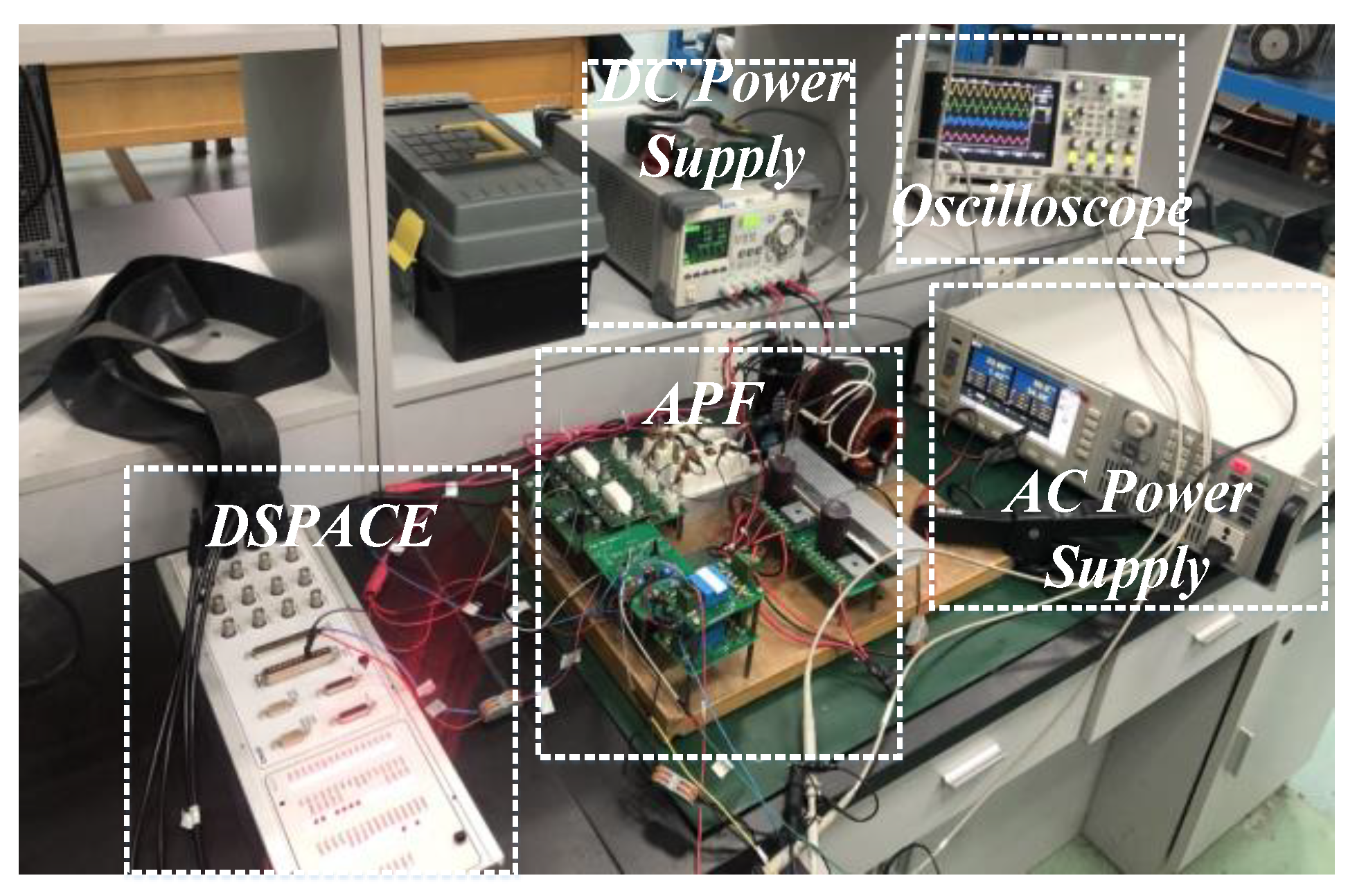
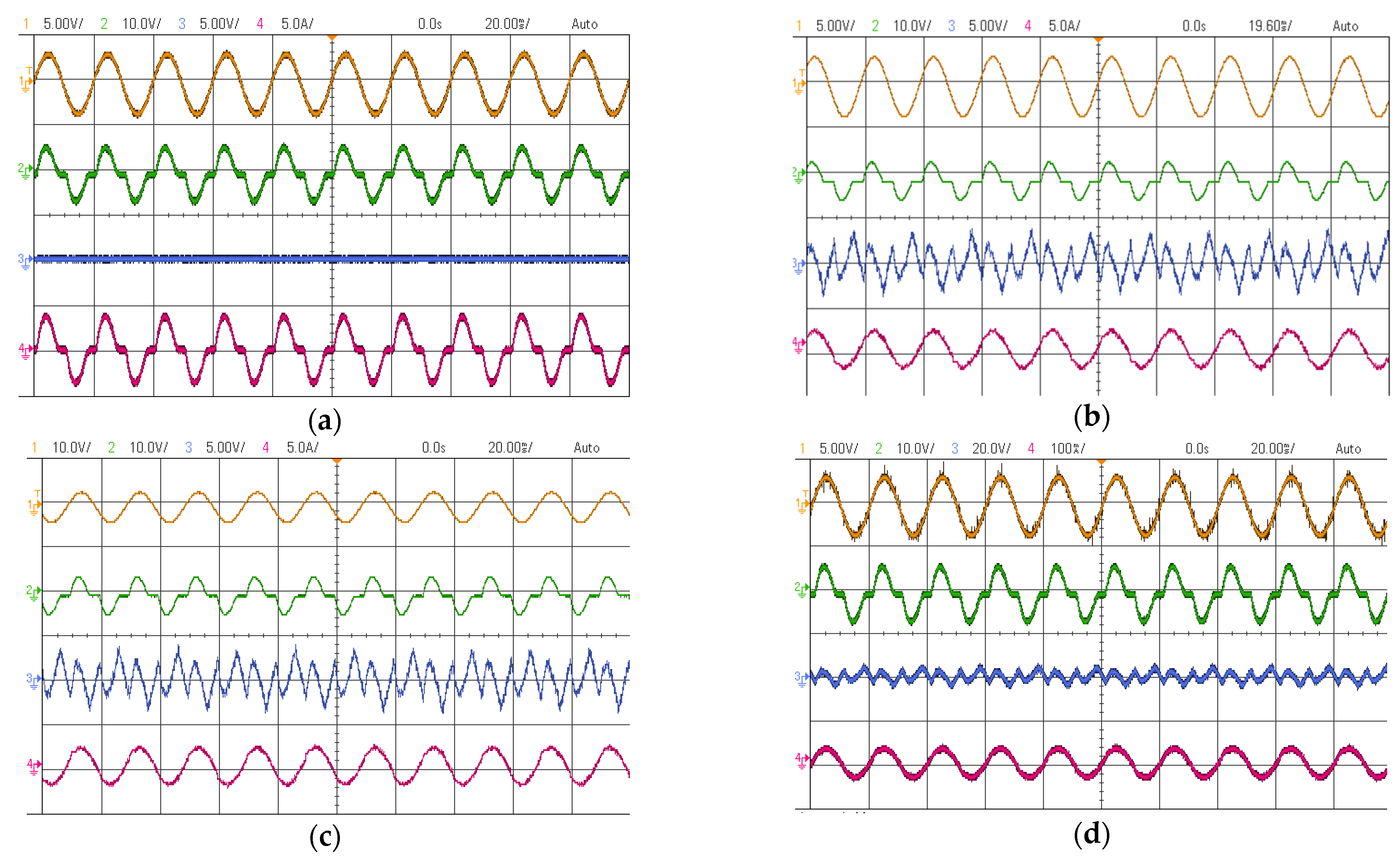
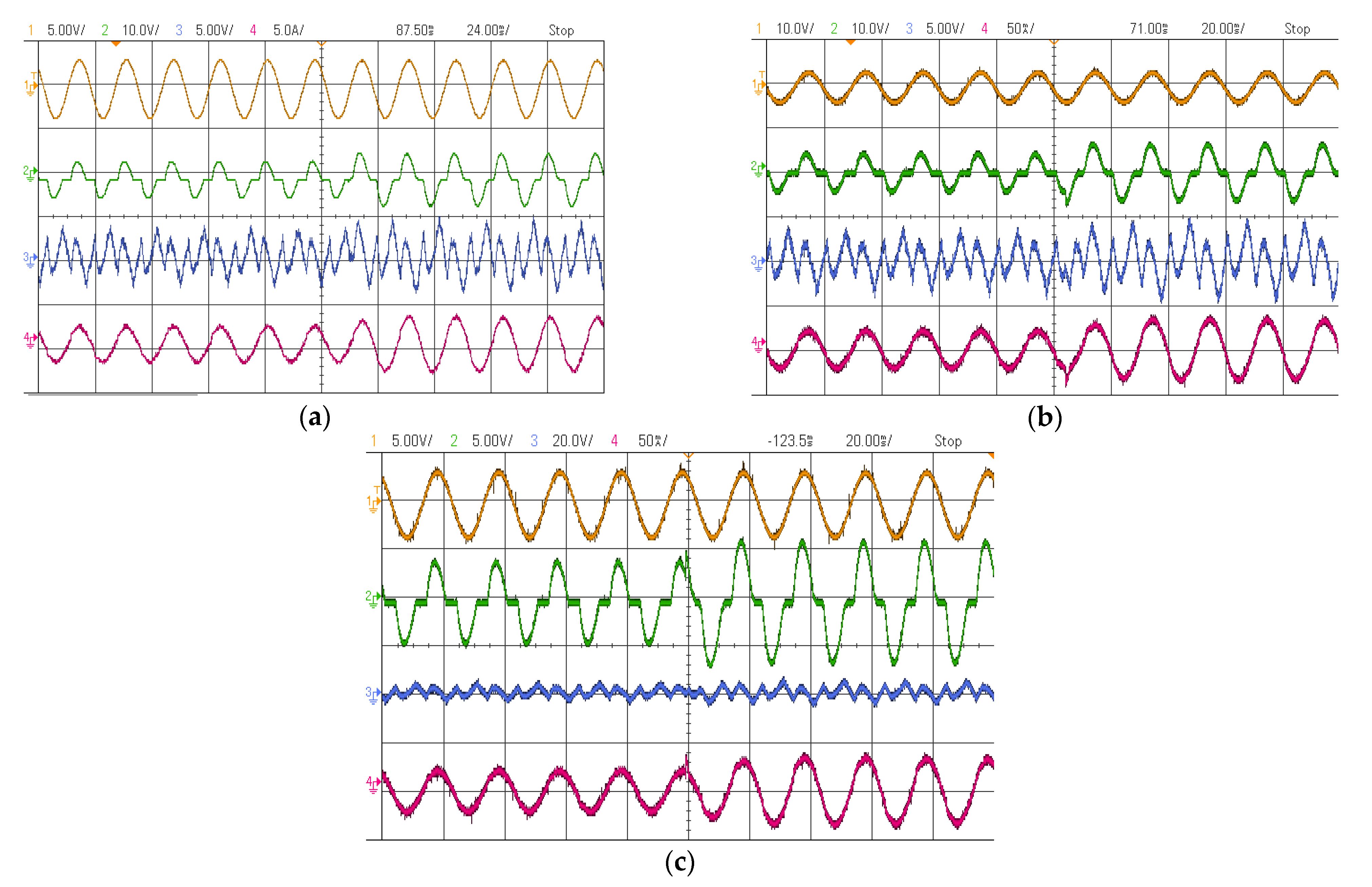
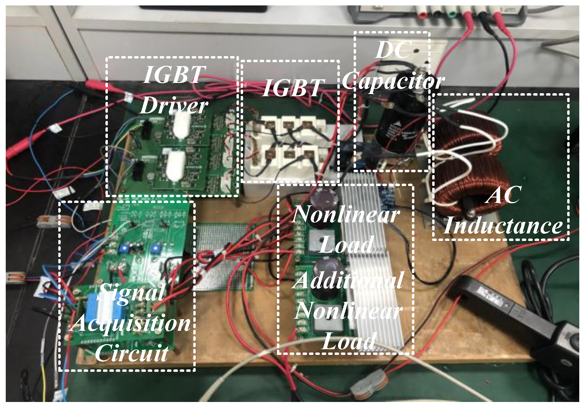
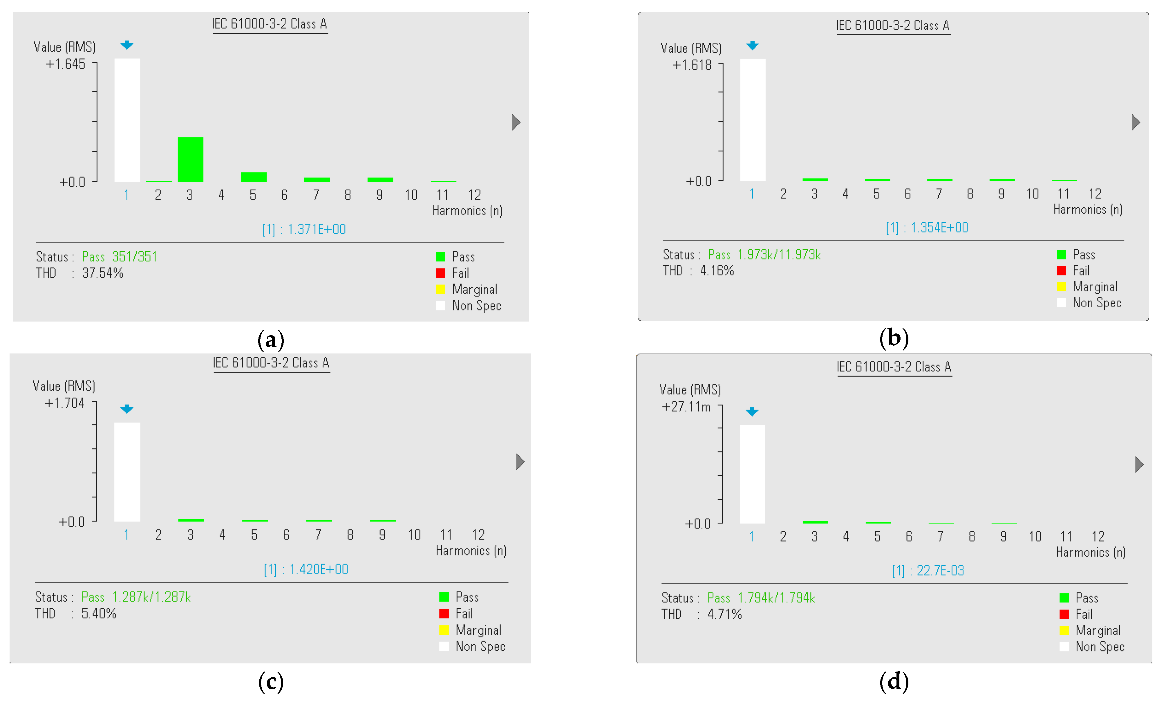
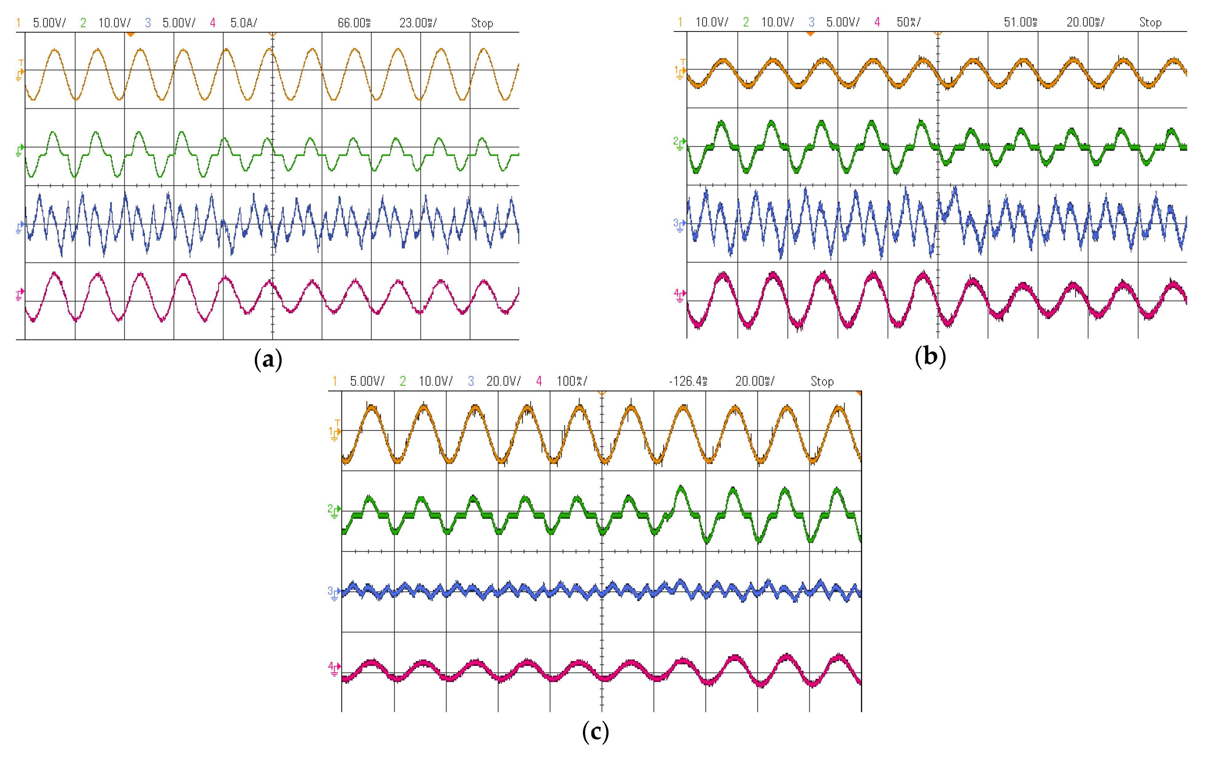
4. Experiment Verification

The efficacy, dependability, and practical feasibility of the innovative control strategy for the APF system are validated through experimental implementation. The following provides an overview of the hardware experiment, including comparative results.

The practical feasibility of the IT2FNN-SFR STSMC is validated using a real-time experimental apparatus for single-phase APF, which is based on the DSPACE DS1104. The parameter of the hardware experiment is given in

Table 1. Parameters in experiment.

Parameters	Values
Supply voltage	$24 \mathsf{V}/50 \mathrm{Hz}$
APF main circuit	$L_c=18 \mathrm{mH}$, $R_c=0.1 \mathsf{\Omega }$, $C_0=2200 \mathsf{\mu }\mathsf{F}$, $U_{dc}^{*}=50 \mathsf{V}$
Nonlinear load at steady state	$R_1=5 \mathsf{\Omega }, R_2=15 \mathsf{\Omega }$, $C_1=1000 \mathrm{uF}$
Additional nonlinear load in parallel	$R_1=15 \mathsf{\Omega }, R_2=15 \mathsf{\Omega }$, $C_2=1000 \mathrm{uF}$
Sampling time	$T_s=50 \mathsf{\mu }\mathsf{s}$

, where the sampling period is $T_s=50 \mathsf{\mu }\mathsf{s}$.

The real-time experimental apparatus is depicted in Figure 4. It can be seen that the implement is composed of an APF circuit module, an AC power supply module, a DC power supply module, a DSPACE control module, and an oscilloscope. As depicted, the APF main circuit, shown in Figure 5, encompasses components such as the IGBT driver, IGBTs, DC capacitor, nonlinear load, additional nonlinear load, and a signal acquisition circuit. The DC power is used to power the IGBT drive. Experimental waveforms and spectrum analyses of the power supply current are captured using the Agilent DSO-X3034A oscilloscope (Keysight Technologies, Santa Rosa, CA, USA). The necessary current and voltage signals are gathered by sensors, and these measured signals are subsequently transmitted to the controller via the A/D converter. The IGBT receives the Pulse Width Modulation (PWM) signal computed by the controller to produce the compensation current.

As shown in Figure 6, the signal waveform curves obtained from the oscilloscope under different methods during stable operation are depicted. The four curves from top to bottom represent the AC power voltage, load current, harmonic compensation current, and AC current, respectively. When the APF is not operational (as shown in Figure 6a), the compensation current is 0 A, indicating severe distortion in the current waveform. Under the influence of different control algorithms (the designed IT2FNN-SFR STSMC, adaptive sliding mode control (ASMC), and traditional super-twisting sliding mode control (STSMC)), compensation of the supply current can be achieved, transforming the distorted waveform into an approximately sinusoidal shape. To further intuitively compare the compensation performance differences among the various methods, a frequency spectrum analysis of the power current is conducted, and the total harmonic distortion (THD) of the supply current under each control method is calculated (results are shown in Figure 7). The results indicate that the harmonic components in the power current are significantly suppressed under the control algorithms. Specifically, the THD corresponding to the control algorithm designed in this paper is improved by 1.24% and 0.55% compared to ASMC and STSMC, respectively, which is below the international standard of 5%.

Remake 1: The harmonic distortion rate is one of the key indicators for assessing the level of harmonics in the power grid. It is typically required to be within a certain range to ensure the stability and normal operation of the power system. According to [29], for generating equipment where the ratio of maximum short-circuit current to maximum demand load current (fundamental component) at the point of common coupling is less than 20, the THD should be kept within 5.0%. Additionally, in [30], the assessment of harmonics is extended to include the limitation of the maximum 50th harmonic, at which point, a sampling period of $50 \mathsf{\mu }\mathsf{s}$ already meets the requirement.

In practice, as the electrical equipment changes, so will the load. Hence, dynamic experiments are formulated to validate the dynamic performance of the devised control method. During the stable operation of the APF system, an additional nonlinear load is introduced to simulate a load collapse. After stable operation, a sudden load increase is simulated by an additional load disconnected in parallel. The results of the dynamic tests are illustrated in Figure 8. It can be observed from the figure that the introduction of additional load results in an increase in the amplitude of both the source current and the load current. It is noteworthy that although the source current under all three control algorithms can recover to a new stable sinusoidal waveform within a relatively short period, the current curve under ASMC control is more prone to sudden changes, which may have adverse effects on the actual operation of the power grid. When the additional load is disconnected, the source current can also recover to a new stable sinusoidal waveform within a short period of time, as shown in Figure 9. Similarly, spectrum analysis is performed on the power supply current with load variation, and the results are listed in

Table 2. Comparison of THD under the three strategies.

	ASMC	STSMC	IT2FNN-SFR STSMC
Steady state	5.40%	4.71%	4.16%
Additional load connected	4.94%	4.23%	3.87%
Additional load disconnected	5.87%	5.10%	4.72%

.

In addition, a comparison of the THD rates in the hardware experiment under the two methods is given in Table 2. It is obvious that the compensation performance of the designed controller is better than ASMC and STSMC in terms of steady state and dynamic response, and it meets the international standard of THD of less than 5% in each state. STSMC, owing to the incorporation of a super-twisting term, enables the continuous switching of the controller, facilitating the rapid convergence of the system on the sliding surface. Compared to ASMC, it reduces the dwell time of the system on the sliding surface, thereby enhancing control efficiency. Hence, the THD under the STSMC algorithm is lower. Additionally, the introduction of IT2FNN-SFR allows for the pre-estimation of the dynamic equations of the APF system, reducing current distortion resulting from external disturbances and further enhancing the robustness of the controller. Based on the aforementioned hardware experimental results, it is evident that the control strategy proposed in this paper meets the control requirements, and its feasibility is demonstrated.

5. Conclusions

This paper presents an adaptive super-twisting sliding mode control (STSMC) strategy for a single-phase active power filter (APF), which integrates an interval type-2 fuzzy neural network (IT2FNN) with a self-feedback recursive structure. The proposed controller effectively addresses the challenges of harmonics suppression in APF systems by approximating the unknown system model using the IT2FNN. By leveraging interval type-2 fuzzy membership functions and historical information, the network enhances its nonlinear processing capability and accuracy, thereby improving the controller’s approximation ability. Moreover, the adaptive STSMC reduces the chattering phenomenon and simplifies parameter setting by incorporating an adaptive law for network parameters. The stability of the system is rigorously established using the Lyapunov method, ensuring reliable performance in practical applications. The experimental results validate the significant improvement in the total harmonic distortion (THD) rate compared to traditional adaptive sliding mode control and super-twisting sliding mode control, demonstrating commendable steady-state performance and dynamic response. It can be inferred that the controller effectively suppresses harmonics in the APF system, highlighting its potential for real-world implementation and contributing to the advancement of power quality improvement techniques.

References

1. Wang, R.; Huang, W.; Hu, B.; Du, Q.; Guo, X. Harmonic Detection for Active Power Filter Based on Two-Step Improved EEMD. IEEE Trans. Instrum. Meas. 2022, 71, 1–10. [Google Scholar] [CrossRef]
2. Mishra, A.K.; Das, S.R.; Ray, P.K.; Mallick, R.K.; Mohanty, A.; Mishra, D.K. PSO-GWO Optimized Fractional Order PID Based Hybrid Shunt Active Power Filter for Power Quality Improvements. IEEE Access 2020, 8, 74497–74512. [Google Scholar] [CrossRef]
3. Noureddine, K.; Abedlhafid, S. ADALINE Harmonics Extraction Algorithm of Three-Level Shunt Active Power Filter Based on Predictive Current Control. In Proceedings of the 2020 International Conference on Electrical Engineering (ICEE), Istanbul, Turkey, 25–27 September 2020; pp. 1–7. [Google Scholar]
4. Mousavi, Y.; Bevan, D.; Kucukdemiral, I.; Fekih, A. Sliding mode control of wind energy conversion systems: Trends and applications. Renew. Sustain. Energy Rev. 2022, 167, 112734. [Google Scholar] [CrossRef]
5. Qu, L.; Qiao, W.; Qu, L. An Extended-State-Observer-Based Sliding-Mode Speed Control for Permanent-Magnet Synchronous Motors. IEEE J. Emerg. Sel. Top. Power Electron. 2021, 9, 1605–1613. [Google Scholar] [CrossRef]
6. Fei, J.; Wang, Z.; Pan, Q. Self-Constructing Fuzzy Neural Fractional-Order Sliding Mode Control of Active Power Filter. IEEE Trans. Neural Netw. Learn. Syst. 2023, 34, 10600–10611. [Google Scholar] [CrossRef] [PubMed]
7. Fei, J.; Xin, M. Robust Adaptive Sliding Mode Controller for Semi-active Vehicle Suspension System. Int. J. Innov. Comput. Inf. Control 2012, 8, 691–700. [Google Scholar]
8. Fei, J.; Zhang, L. Self-Constructing Chebyshev Fuzzy Neural Complementary Sliding Mode Control and Its Application. IEEE Trans. Neural Netw. Learn. Syst. 2024, 1–14. [Google Scholar] [CrossRef] [PubMed]
9. Lin, X.; Liu, J.; Liu, F.; Liu, Z.; Gao, Y.; Sun, G. Fractional-Order Sliding Mode Approach of Buck Converters with Mismatched Disturbances. IEEE Trans. Circuits Syst. I Regul. Pap. 2021, 68, 3890–3900. [Google Scholar] [CrossRef]
10. Fei, J.; Wang, H.; Fang, Y. Novel Neural Network Fractional-order Sliding Mode Control with Application to Active Power Filter. IEEE Trans. Syst. Man Cybern. Syst. 2022, 52, 3508–3518. [Google Scholar] [CrossRef]
11. Hou, Q.; Ding, S.; Yu, X. Composite Super-Twisting Sliding Mode Control Design for PMSM Speed Regulation Problem Based on a Novel Disturbance Observer. IEEE Trans. Energy Convers. 2021, 36, 2591–2599. [Google Scholar] [CrossRef]
12. Zholtayev, D.; Rubagotti, M.; Do, T.D. Adaptive super-twisting sliding mode control for maximum power point tracking of PMSG-based wind energy conversion systems. Renew. Energy 2022, 183, 877–889. [Google Scholar] [CrossRef]
13. Wu, Y.; Ma, F.; Liu, X.; Hua, Y.; Liu, X.; Li, G. Super Twisting Disturbance Observer-Based Fixed-Time Sliding Mode Backstepping Control for Air-Breathing Hypersonic Vehicle. IEEE Access 2020, 8, 17567–17583. [Google Scholar] [CrossRef]
14. Shah, I.; Rehman, F. Smooth Second Order Sliding Mode Control of a Class of Underactuated Mechanical Systems. IEEE Access 2018, 6, 7759–7771. [Google Scholar] [CrossRef]
15. Fei, J.; Chen, Y.; Liu, L.; Fang, Y. Fuzzy Multiple Hidden Layer Recurrent Neural Control of Nonlinear System Using Terminal Sliding-Mode Controller. IEEE Trans. Cybern. 2022, 52, 9519–9534. [Google Scholar] [CrossRef] [PubMed]
16. Liu, Y.; Su, C.; Li, H.; Lu, R. Barrier Function-Based Adaptive Control for Uncertain Strict-Feedback Systems Within Predefined Neural Network Approximation Sets. IEEE Trans. Neural Netw. Learn. Syst. 2020, 31, 2942–2954. [Google Scholar] [CrossRef] [PubMed]
17. Deng, F.; Hua, M. Robust delay-dependent exponential stability for uncertain stochastic neural networks with mixed delays. Neurocomputing 2011, 74, 1503–1509. [Google Scholar] [CrossRef]
18. Sun, Y.; Xu, J.; Lin, G.; Sun, N. Adaptive neural network control for maglev vehicle systems with time-varying mass and external disturbance. Neural Comput. Appl. 2023, 35, 12361–12372. [Google Scholar] [CrossRef]
19. Xiao, J.; Cheng, J.; Shi, K.; Zhang, R. A General Approach to Fixed-Time Synchronization Problem for Fractional-Order Multidimension-Valued Fuzzy Neural Networks Based on Memristor. IEEE Trans. Fuzzy Syst. 2022, 30, 968–977. [Google Scholar] [CrossRef]
20. Li, Y.; Dong, S.; Li, K. Fuzzy adaptive finite-time event-triggered control of time-varying formation for nonholonomic multirobot systems. IEEE Trans. Intell. Veh. 2023, 9, 725–737. [Google Scholar] [CrossRef]
21. Fei, J.; Liu, L. Real-Time Nonlinear Model Predictive Control of Active Power Filter Using Self-Feedback Recurrent Fuzzy Neural Network Estimator. IEEE Trans. Ind. Electron. 2022, 69, 8366–8376. [Google Scholar] [CrossRef]
22. Xu, B.; Zhang, R.; Li, S.; He, W.; Shi, Z. Composite Neural Learning Based Nonsingular Terminal Sliding Mode Control of MEMS Gyroscopes. IEEE Trans. Neural Netw. Learn. Syst. 2020, 31, 1375–1386. [Google Scholar] [CrossRef] [PubMed]
23. Zhao, T.; Liu, J.; Dian, S.; Guo, R.; Li, S. Sliding-Mode-Control-Theory-Based Adaptive General Type-2 Fuzzy Neural Network Control for Power-line Inspection Robots. Neurocomputing 2020, 401, 281–294. [Google Scholar] [CrossRef]
24. Du, G.; Liang, Y.; Gao, B.; Al Otaibi, S.; Li, D. A Cognitive Joint Angle Compensation System Based on Self-Feedback Fuzzy Neural Network with Incremental Learning. IEEE Trans. Ind. Inform. 2021, 17, 2928–2937. [Google Scholar] [CrossRef]
25. Li, Y.; Feng, K.; Li, K. Finite-time fuzzy adaptive dynamic event-triggered formation tracking control for USVs with actuator faults and multiple constraints. IEEE Trans. Ind. Inform. 2023, 20, 5285–5296. [Google Scholar] [CrossRef]
26. Kumar, R.; Srivastava, S. A novel dynamic recurrent functional link neural network-based identification of nonlinear systems using Lyapunov stability analysis. Neural Comput. Appl. 2021, 33, 7875–7892. [Google Scholar] [CrossRef]
27. Cheng, T.; Wu, J.; Wang, H.; Zheng, H. Dynamic Optimization of Rotor-Side PI Controller Parameters for Doubly-Fed Wind Turbines Based on Improved Recurrent Neural Networks Under Wind Speed Fluctuations. IEEE Access 2023, 11, 102713–102726. [Google Scholar] [CrossRef]
28. Wang, J.; Fang, Y.; Fei, J. Adaptive Super-Twisting Sliding Mode Control of Active Power Filter Using Interval Type-2-Fuzzy Neural Networks. Mathematics 2023, 11, 2785. [Google Scholar] [CrossRef]
29. Blooming, T.M.; Carnovale, D.J. Application of IEEE STD 519-1992 Harmonic Limits. In Proceedings of the Conference Record of 2006 Annual Pulp and Paper Industry Technical Conference, Appleton, WI, USA, 18–22 June 2006; pp. 1–9. [Google Scholar]
30. Wallace, I. Key Changes and Differences between the New IEEE 519-2014 Standard and IEEE 519-1992. Alcatel Telecommun. Rev. 2014, 11, 1–2. [Google Scholar]
Figure 1. The schematic representation of a single-phase active power filter.
Applsci 14 03271 g001
Figure 2. The schematic diagram of IT2FNN-SFR STSMC.
Applsci 14 03271 g002
Figure 3. The architecture of IT2FNN-SFR.
Applsci 14 03271 g003
Figure 4. The APF real-time experimental apparatus.
Applsci 14 03271 g004
Figure 5. The intricate main circuit module of APF.
Applsci 14 03271 g005
Figure 6. Curves of power supply voltage, load current, compensation current, and power supply current measured at steady state under different methods: (a) no compensation algorithm is applied; (b) IT2FNN-SFR STSMC algorithm; (c) ASMC algorithm; (d) traditional STSMC algorithm.
Applsci 14 03271 g006
Figure 7. Comparison of THD at steady state under different methods: (a) no compensation algorithm is applied; (b) IT2FNN-SFR STSMC algorithm; (c) ASMC algorithm; (d) traditional STSMC algorithm.
Applsci 14 03271 g007
Figure 8. Curves of power supply voltage, load current, compensation current, and power supply current measured when the additional load is connected under different methods: (a) IT2FNN-SFR STSMC algorithm; (b) ASMC algorithm; (c) traditional STSMC algorithm.
Applsci 14 03271 g008
Figure 9. Curves of power supply voltage, load current, compensation current, and power supply current measured when the additional load is disconnected under different methods: (a) IT2FNNSFR STSMC algorithm; (b) ASMC algorithm; (c) traditional STSMC algorithm.
Applsci 14 03271 g009