Abstract
The multi-dimensional optimization of mechanisms is a typical optimization problem encountered in mechanical design. Herein, the Hybrid strategy improved Beetle Antennae Search (HSBAS) algorithm is proposed to solve the multi-dimensional optimization problems encountered in structural design. To solve the problems of local optimization and low accuracy of the high-dimensional solution of the Beetle Antennae Search (BAS) algorithm, the algorithm adopts the adaptive step strategy, multi-directional exploration strategy, and Lens Opposition-Based Learning strategy, significantly reducing the probability of the algorithm falling into the local optimum and improving its global search capability. Comparative experiments of the improved algorithm are carried out by selecting eleven benchmark test functions. HSBAS can reach 1 × 10⁻²² accuracy from the optimal value when dealing with low-dimensional functions. It can also obtain 1 × 10⁻² accuracy when dealing with high-dimensional functions, significantly improving the algorithm’s capability. According to Friedman’s ranking test result, HSBAS ranks first, which proves that HSBAS is superior to the other three algorithms. The HSBAS algorithm is further used to optimize the design of the altitude compensation module of the gravity compensation device for solar wings, controlling the fluctuation of bearing capacity within 0.25%, which shows that the algorithm can be used as an effective tool for engineering structural optimization problems.
1. Introduction
Traditional optimization algorithms, such as the steepest descent method and variable metric method, are gradually unable to meet the needs of engineering optimization as the problems faced by the engineering field are becoming increasingly complex [1]. Recently, intelligent optimization algorithms, as a new evolutionary computational tool, have been widely used in engineering optimization problems [2,3,4]. As one of the heuristic search algorithms, the Beetle Antennae Search (BAS) algorithm enjoys the advantages of fast convergence, simple model, low computational complexity, and robust searching ability [5,6], and is widely employed in several engineering optimization problems with high research value [7,8,9,10].
Until now, many researchers have been making efforts to improve the performance of the BAS algorithm further, and mainstream approaches include the search step-size adjustment and algorithm fusion. Khan et al. [11] proposed a BAS algorithm combined with Adaptive Moment Estimation (ADAM), named BAS-ADAM, aiming to avoid falling into the locally optimal solution, which increases the computational complexity at the cost of time. Wang et al. [12] introduced a Beetle Swarm Antennae Search (BSAS) algorithm combined with step-size self-adjustment, reducing the need to update the step iteratively and improving the ability to solve high-dimensional problems. Li et al. [13] designed a BAS-PSO algorithm combining the BAS algorithm with the Particle Swarm Optimization (PSO) algorithm to enhance the local and global search ability, possibly reducing the convergence rate. Fan et al. [14] proposed a BGWO algorithm that integrates the BAS algorithm with Grey Wolf Optimizer (GWO), which improves the local optimum situation caused by the lack of population diversity and the problem of group hierarchical structure in GWO, thus enhancing search efficiency and robustness. Moreover, there are variations in the algorithm based on Lévy flight, adaptive mechanism, quadratic interpolation [15,16,17], etc.
BAS algorithms are widely used in engineering applications. Zhu et al. [18] constructed a multi-objective optimization model for microgrids based on BAS to minimize operation and pollution treatment costs; Xie et al. [19] developed an improved BAS algorithm for collision prediction and obstacle avoidance of underdriven ships; and Li et al. [20] combined an augmented selection mechanism, a deep learning algorithm, and BAS to improve the accuracy of BAS in the fault diagnosis of rolling bearings. Zhang et al. [21] employed the BAS algorithm with Lévy flight and inertia weight optimization to tune the hyperparameters in random forests, optimizing the resume design of reinforced concrete beams. Khan et al. [22] investigated a binarized BAS algorithm to increase the diversity of tangential portfolios. Wang et al. [23] combined BAS with the Radial Basis Function Neural Network to model the friction characteristics of robot joints.
Based on the No Free Lunch Theorem, no optimization algorithm can solve all optimization problems. For some applications, a metaheuristic may provide prosperous solutions, while it may provide poor performance for other applications [24]. In this paper, a Hybrid Strategy Improved Beetle Antennae Search (HSBAS) algorithm is adopted to solve the multi-dimensional optimization problem in engineering mechanisms. In the initial stage of the algorithm, the step is updated appropriately and explored in multiple directions to strengthen the global optimization ability; meanwhile, the Lens Opposition-Based Learning is interspersed to improve the sample diversity. By comparing and calibrating with other algorithms widely used in engineering structural design, the superiority of HSBAS is verified. Meanwhile, it is further applied to the altitude compensation module of a solar wing-based gravity unloading device to verify its effectiveness in engineering practice. The effectiveness and applicability of HSBAS in practical structural design problems are verified.
2. Beetle Antennae Search algorithm
The Beetle Antennae Search algorithm is inspired by the predation of Beetle, namely, through the left and right antennae on the head of the Beetle to sense the strength of the food flavor to determine the direction of the flight, and finally find the exact location of the food [25], as shown in Figure 1.
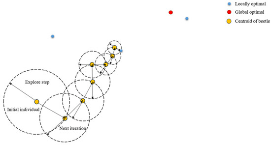
Figure 1.
Schematic diagram of standard Beetle Antennae Search algorithm search process.
The optimization process of the practical problem is abstracted into the process of antennae foraging, and the parameter that needs to be solved in the practical problem, i.e., the optimal solution, is regarded as the location of the center of mass of the beetle in the n-dimensional space, and the optimization process is as follows:
- 1.
- Setting the direction of antennae whiskers . It is represented by a random unit vector and normalized by [25],
- 2.
- Setting the step factor. is the exploration step length at the iteration, and the step length mainly determines the search capability of antennae whiskers [25],
- 3.
- Establishing the location coordinates of the left and right antennae whiskers [25].
- 4.
- Updating the mass center position of the new antennae.
- 5.
- The location of the antennae at the next iteration (the iteration) is selected based on the food smell concentration of the antennae’s left and right whiskers (the magnitude of the objective function value ) [25]:
3. Hybrid Strategy Improved Beetle Antennae Search Algorithm
The Beetle Antennae Search algorithm is a single search algorithm with the advantages of low computational complexity, low spatial complexity, and fewer required parameters than other intelligent algorithms. The Beetle Antennae Search algorithm shows good optimization speed and accuracy when dealing with low-dimensional optimization problems and is widely used in continuous variable optimization problems. However, when dealing with high-dimensional problems, it is easy to fall into local optimal solutions, limiting its practical application. The primary causes are the rapid decrease in the step and the limited exploration direction of the Beetle Antennae Search algorithm.
This study proposes the Hybrid Strategy Improved Beetle Antennae Search algorithm (HSBAS) to address the above problems. We balance the algorithm’s global search capability and local exploration capability with the adaptive step length strategy, the multi-direction exploration strategy, and the transitive reverse learning strategy while maintaining the computational efficiency of the algorithm. These strategies improve the global exploration ability in the initial stage of the algorithm and expand the search scope by using the reverse learning strategy when the algorithm has repeated optimal solutions.
3.1. Adaptive Step Strategy
The performance of the Beetle Antennae Search algorithm is mainly decided by the step factor of Beetle Antennae based on the principle of the BAS algorithm. If the search step of the Antennae whisker decays slowly enough, the global search capability will be more substantial, but the convergence speed will be slower. On the contrary, if the search step decays too fast, the algorithm may converge before finding the global optimal solution. Therefore, a balance between global search capability and convergence speed is needed to ensure practical exploration and prevent premature convergence.
To balance the global search capability and convergence ability, this study proposes an adaptive step strategy to update the step length at an appropriate time in the initial stage of the algorithm. The strategy is as follows: an exploration step count and an exploration step threshold are introduced into the Beetle Antennae Search algorithm. We first judge whether the last exploration step is smaller than in the iterative process. If yes, it indicates that the algorithm is already in the small convergence search stage, so we need to increase the exploration step length to jump out of the local optimum. An exploration step counter and a maximum exploration step lengthening number are also introduced to prevent the algorithm from converging poorly. Every time the step grows, increases by 1, and when is larger than , the exploration step lengthening mechanism fails; meanwhile, the algorithm enters a small-scale convergence search stage and converges near the global optimum until the global optimal solution is found.
The step update formula is as follows: when or , the position update formula follows the step length update formula of the original Beetle Antennae Search algorithm; when and , the following step length update and position update formulas are used.
where is the step length set at the beginning; is the length of the step at the antenna exploration; and is the step updating factor, it indicates that the variable step length decreases gradually with the number of iterations increases, and can be selected according to the complexity of the requested problem.The value of ranges from 0.99 to 1, and . The value of is selected by judging the dimension and complexity of the problem; when solving high-dimensional complex problems, the value of is larger, ranging from 150 to 200; when dealing with low-dimensional simple problems, the value of is smaller, ranging from 75 to 150. The value of balances the relationship between exploration and convergence abilities. The algorithm converges fast when dealing with low-dimensional problems and converges slowly when dealing with high-dimensional problems with a large exploration range. The value of the is determined by the original BAS algorithm step, generally between 0.6 and 0.8 times. Hence, the algorithm avoids entering the fast convergence phase.
3.2. Multi-Directional Exploration Strategy
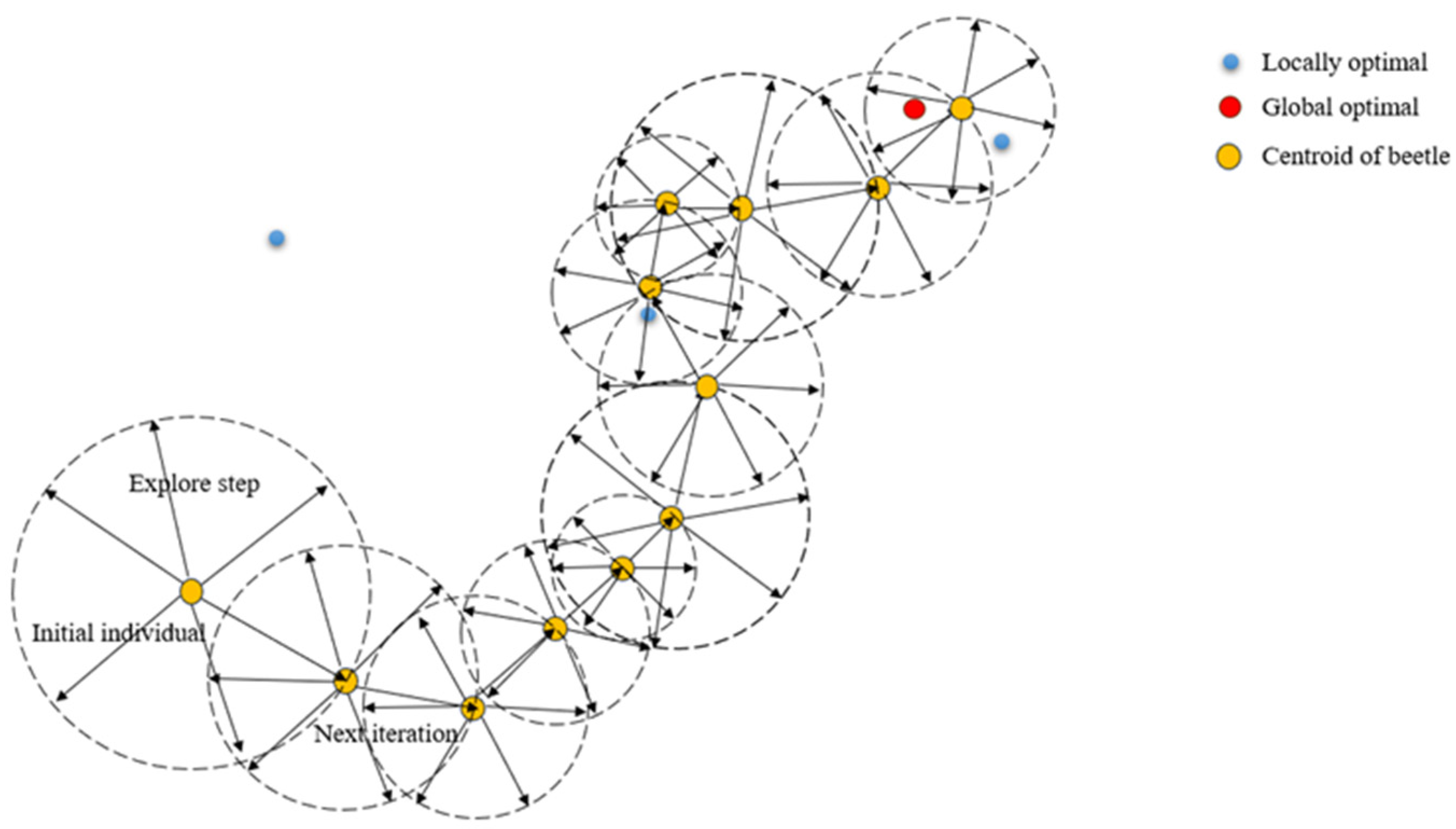
The original Beetle Antennae Search algorithm has a limited exploration capability because it only randomly explores two symmetric directions. It increases the risk of ignoring the optimal solution near the given point; the exploration of the algorithm has some defects. To enhance the global search capability of the algorithm, this study proposes a multi-directional search strategy at the initial stage of the algorithm. This strategy enables the antennas to explore multiple directions concurrently to expand the detection range. In the late stage of the algorithm, the multi-directional search strategy is stopped to reduce the algorithm’s complexity, as shown in Figure 2. The multi-directional exploration formula is as follows:
where indicates that pairs of n-dimensional vectors are randomly generated, and indicates that pairs of exploration directions are generated. Antennae whiskers need to explore in directions. If the value of is set too large, it will increase the algorithm’s complexity, which is harmful to the algorithm’s convergence. If it is set too small, it harms the exploration of the algorithm. The range of the value of can be taken from 4 to 6, and the specific value can be analyzed according to the specific situation.
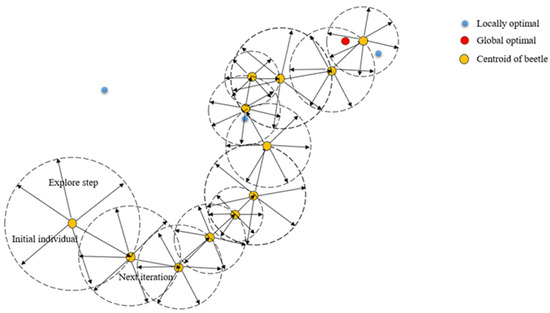
Figure 2.
Schematic diagram of the search process of Beetle Antennae Search algorithm after adaptive step length and multi-directional exploration improvement.
The position of the individual beetle can be further updated as the following equation:
where denotes the row of , the direction of exploration of the beetle antennae, and is substituted into the equation of position update.
3.3. Lens Opposition-Based Learning Strategy
Opposition-Based Learning (OBL) selects the better of the two to propagate through subsequent iterations by evaluating both the current solution and its inverse at each iteration. In a study examining heuristic optimization techniques, Rahnamayan et al. [26] demonstrated that the probabilistic likelihood of an inverse solution residing closer to the global optimum target is greater than that of the existing iterated solution. By exploiting the higher quality of inverse solutions, reverse learning can effectively enhance algorithm performance [27].
Lens Opposition-Based Learning (LOBL) marries inverse learning approaches with optical lens inversion physics to dynamically redirect optimization value from local extrema [28,29]. Specifically, when converging upon suboptimal solutions, LOBL evaluates the “inverse image” solution through a computational inversion “lens”. Specifically, when converging upon suboptimal solutions, LOBL evaluates the “inverse image” solution through a computational inversion “lens”, as shown in Figure 3. Better solutions become visible by comparing iterative improvements from current versus inverted vectors. The strategy increases the diversity of solutions, avoids local optimization, and improves the global optimization ability of the algorithm. It is combined with various algorithms successfully to improve the algorithm’s optimization ability significantly [30].
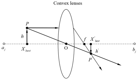
Figure 3.
Schematic diagram of Lens Opposition process.
In the search space of the optimization issue, let the position of the global optimal solution be , which is determined by the projection of the individual on the x-axis. The lower bound and the upper bound represent the dimensional value range of the coordinates. The convex lens with focal length f is placed at the coordinate origin . Individual is refracted and imaged by the lens, and the image point with height is obtained. As a result, the opposite point corresponding to the global optimal solution obtained by lens reflection is formed on the x-axis. According to the principle of lens imaging, it can be obtained as follows [28,29],
Setting , the expression , is obtained by transforming as follows [28,29]:
When takes the value of 1, the formula of LOBL can be simplified to the formula of OBL. The inverse solution obtained by general inverse learning is fixed. In contrast, the inverse solution obtained by transmission inverse learning can be dynamically varied by changing the value of , further improving the global optimization ability of the algorithm. In addition, a smaller value of will generate a broader range of inverse solutions, and a larger value of will generate a smaller range of inverse solutions. Considering that the optimization algorithm typically performs a large-scale search followed by a local delicate search, the dynamic change in is introduced in this study:
As the number of iterations increases, the value of will become larger and the range of its inverse solution will become smaller.
The specific process of the algorithm is shown in Algorithm 1.
| Algorithm 1: HSBAS algorithm |
| Begin Input: Fitness function Initialize the parameters Output: the best solution x* and the best value of fitness function. While (t < Tmax do If , then Generate the step according to (6) End Generate the direction vector unit according to (7) Generate multiple explore direction randomly according to (8) If then, End If is an even number, Lens Opposition-Based Learning according to (10) Compare the Fitness function value; update the best value and position. if , then, End End End Update sensing diameter d and step length with decreasing functions (4) and (5), respectively; End Return |
4. Simulation Experiment and Analysis
4.1. Algorithm Data Comparison
To quantitatively evaluate the performance of the Hybrid Strategy Improved Beetle Antennae Search (HSBAS) algorithm, the study conducted simulation experiments on ten selected standard test functions, as shown in Table 1. Among the selected test functions, belong to the single-peak function, which has only a single extreme point in the definition domain, and the use of such functions to evaluate the algorithm can test its convergence rate and optimization search accuracy, thus reflecting the optimization performance level of the algorithm. Moreover, belongs to the multi-peak function, and belong to the fixed-dimension multi-peak function, with multiple extreme points, usually used to evaluate the algorithm’s performance in the global search ability and avoid premature convergence.

Table 1.
Eleven benchmark test functions.
The simulation experiments were conducted on a computer with 64-bit Windows operating system, Intel® Core (TM) i7-10870H CPU @ 2.20 GHz 2.21 GHz processor (Intel, Santa Clara, CA, USA), 16 G RAM (LC Power, Willich, Germany), and the algorithms were implemented using software MATLAB R2016b. A single execution was run 1000 times, and each algorithm ran 30 experiments independently for each test function. Set the species dimension to 30 for PSO and GA and set the species dimension to 1 for BAS and HSBAS. Their means and standard deviations were recorded separately, as shown in Table 2.
Table 2.
Comparisons of HSBAS and three other algorithms for 11 test functions.
The superiority of HSBAS is verified compared to other algorithms widely used in engineering structure optimization. The HSBAS algorithm shows better stability and optimization search ability in optimizing high-dimensional functions and achieves better optimal function values than the BAS algorithm. Compared with PSO and GA algorithms, HSBAS performs better on nine optimization functions and only shows sub-optimal performance on and . Friedman’s ranking test results show that HSBAS is ranked first, PSO is ranked second, GA is ranked third, and BAS is fourth. The results indicate that the HSBAS algorithm effectively improves its performance in high-dimensional function optimization by improving the algorithm structure and parameter settings, overcoming the BAS algorithm’s local optimum and stability problems. In contrast, when dealing with optimization problems, the PSO and GA algorithms have strong global searching abilities with weak local searching abilities, which may lead to the premature maturity.
4.2. Convergence Analysis of Algorithms
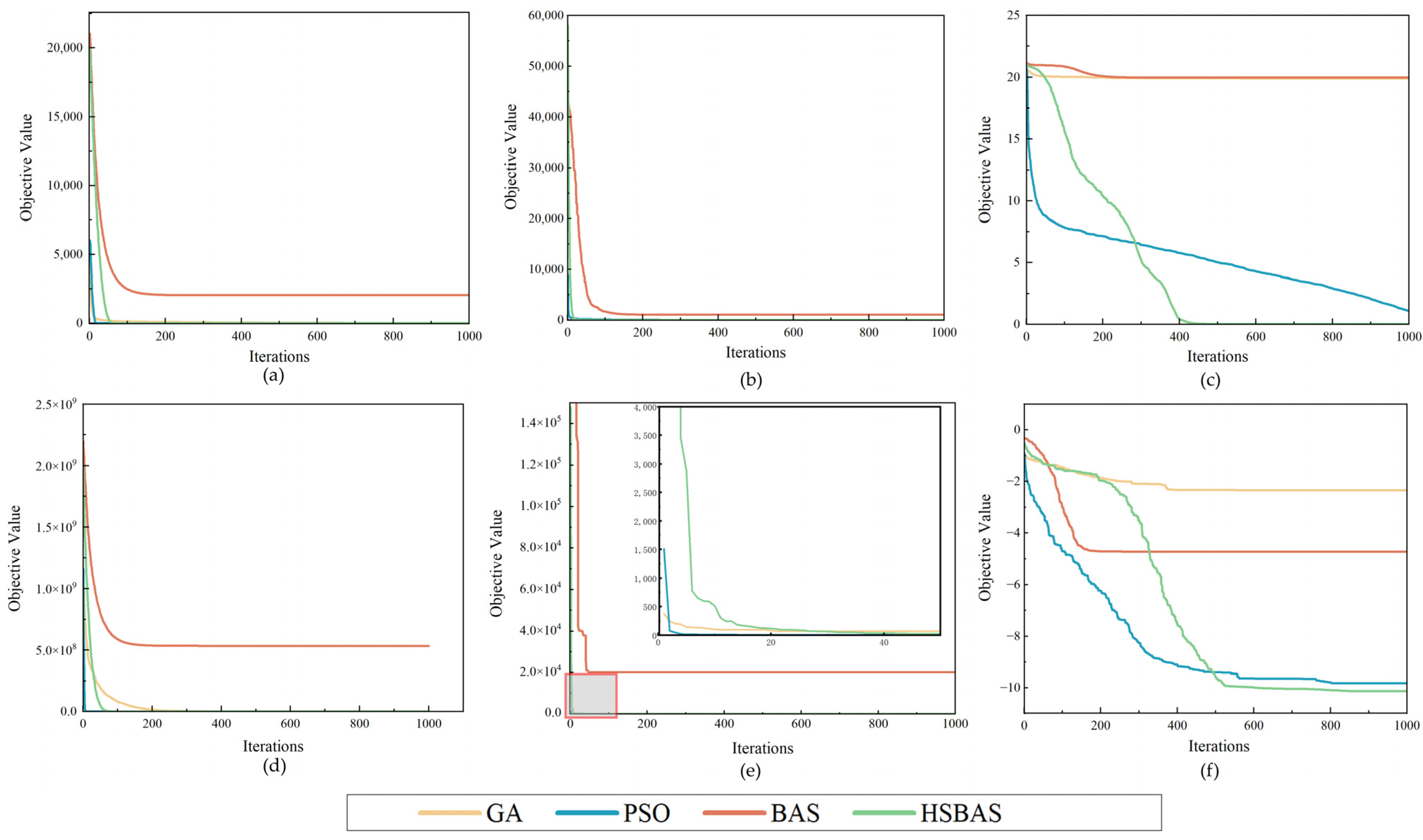
To further verify the convergence performance of the HSBAS algorithm, Figure 4 gives the convergence curves of HSBAS, BAS, and PSO, GA algorithms for some representative standard test functions in Table 2. Setting the population size of PSO and GA algorithms to 30, and the maximum number of function evaluations to 1000, the performance of each intelligent algorithm for single-peak test function, multi-peak test function, and fixed-dimension multi-peak test function can be reflected intuitively.
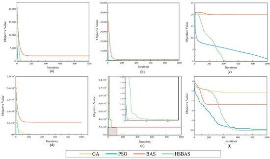
Figure 4.
Convergence curves of HSBAS, BAS, PSO, and GA algorithms on representative standard test functions. (a) ; (b) ; (c) ; (d) ; (e) ; (f) .
According to Figure 4, when dealing with low-dimensional functions, HSBAS algorithm retains the advantage of BAS algorithm in convergence speed, entering the convergence stage in less than 40 steps and obtaining better optimization results; when dealing with ordinary high-dimensional functions, HSBAS algorithm also shows a fast convergence speed and enters the convergence stage in about 30 steps; when dealing with multi-peak functions, HSBAS algorithm enters the convergence stage in less than 500 steps owing to the need to jump out of the local optimum several times. However, it facilitates better jumping out of the local optimum and obtaining better objective function values. Comparing the performance of PSO and GA algorithms, the PSO algorithm achieves good optimization results and convergence speed in most functions. However, it enters the convergence stage more slowly and has worse optimization results when dealing with multi-peak functions. In a comprehensive comparison, the HSBAS algorithm performs well on both low-dimensional and high-dimensional functions, with moderate convergence speed and good optimization results, especially in jumping out of the local optimum.
4.3. Computational Complexity Analysis of Algorithms
The computational complexity of the HSBAS algorithm is mainly composed of three parts: the adaptive step strategy, the multi-directional exploration strategy, and the Lens Opposition-Based Learning strategy. Assuming that the dimension of the solution problem is D, the number of iterations is T, and the directions of the multi-direction exploration strategy is K, the computational complexity of the adaptive step updating strategy and the maximum computational complexity of the multi-direction exploration strategy can be expressed as together. As the Lens Opposition-Based Learning strategy executes alternately, the computational complexity of the Lens Opposition-Based Learning strategy can be denoted as . The computational complexity of the HSBAS algorithm can be derived as follows:
The computational complexity of the standard BAS can be expressed as follows,
Assuming that the number of populations is N, the computational complexity of the standard PSO algorithm can be expressed as follows,
Assuming that the chromosome length is P, the computational complexity of the standard GA algorithm can be expressed as follows,
The number of selected populations N is 30, and the number of directions of the multi-directional exploration strategy K is 3. Therefore, a comprehensive comparison of the algorithm computational complexity yields . The HSBAS algorithm adds some computational amount to the BAS algorithm but is much better at jumping out of the local optimum and improves the performance of the algorithm. Compared to PSO and GA algorithms, it outperforms GA in calculating the optimal solutions of most algorithms and obtains a similar performance to PSO. In terms of computational complexity, it outperforms both of the algorithms.
5. Application to Mechanical Module Design
This study applies the Hybrid Strategy Improved Beetle Antennae Search (HSBAS) algorithm to optimize the design of the altitude compensation module in the gravity compensation device for solar wings to further verify the value of the algorithm for engineering applications. To evaluate the effectiveness of the proposed algorithm, this study conducted comparative experiments between the algorithm and the traditional Beetle Antennae Search (BAS) algorithm, Genetic Algorithm (GA), and Particle Swarm Optimization (PSO) algorithm on the same problem. In addition, the penalty function method is used to constrain the algorithm effectively for the transgressive solutions that the algorithm is prone to produce under existing constraints.
5.1. Physical and Mathematical Modeling of the Height Compensation Module
The altitude compensation module is obtained using the synergistic design of the linkage mechanism, constant force coil spring, grooved roller, spring set, and symmetric support. Specifically, as shown in Figure 5, the T-rail on the load platform cooperates with the roller mounted at point A to form a recess. The connecting rods and take points and as the rotation centers, respectively; , , and are the hinge points. The bottom of the load platform is equipped with a parallel structure of adjustable stiffness as a spring set, with the springs of different stiffnesses arranged in parallel to realize the adjustability of the overall stiffness. Considering that the altitude compensation module needs to compensate for the gravity of solar wing dynamically and cannot provide constant friction, the structural parameters need to be optimized using the intelligent optimization algorithm to make the output of the compensation module stable at about 500 N load.
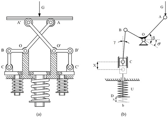
Figure 5.
The two-dimensional simplified model of the altitude compensation module structure. (a) Physical model; (b) mathematical model.
Because of the symmetrical design of the height compensation module, the mechanical analysis of the rod combination is carried out first to reduce the calculation steps.
The torque-equilibrium equation for the rotation center can be expressed as follows,
where is the altitude compensation module load on the platform; and are the lengths of both sides of the connecting rod, respectively; is the outer angle of the connecting rod ; is the arbitrary angle of rotating around ; is the force of the connecting rod on the connecting rod ; and is the angle of the connecting rod and the plumbline, when the altitude compensation module is in the initial working state, is 0.
The expression of the bearing capacity can be obtained after substituting the analysis of the elastic force and the vertical force.
where is the stiffness of the compression spring U; is the new compression of the compression spring after rotating the connecting rod by the angle ; and is the preload value of the compression spring in the initial operating state.
The expressions for and can be obtained by geometrically analyzing the model of the height compensation module.
where is the length of the connecting rod .
Taking the gravity of the rod into account in the load and coupling the above three equations,
where is the self-weight of the top loading platform; and are the self-weights of the and sections of the connecting rod ; and and are the self-weights of the spring-loaded support and the rod , respectively.
Let , , the final load equation of the altitude compensation module is obtained as,
According to Equation (4), after the structural parameters of the altitude compensation module are determined, its load-carrying capacity is not a fixed value but a function of the operating state’s rotation angle.
This paper introduces a kind of index—the squares deviation , which is used to judge the advantages and disadvantages of the design of the altitude compensation module, and to make the squares deviation as small as possible, the design needs to be optimized by the optimization of the altitude compensation module.
where and are the maximum load and minimum load of the height compensation module in the work stroke, respectively; and is the target load.
According to the design requirements, the adaptability function value is obtained,
Because of the wading limit and travel limit, as well as the condition that each parameter cannot be negative, the constraints are obtained,
where the is the upward rounding of the maximum rotation angle of the connecting rod .
5.2. Constraint Treatment
An optimization problem with constraints can be transformed into an unconstrained optimization problem by the penalty function or constraint handling method when solving optimization problems using intelligent algorithms [22]. The penalty function method is one of the commonly adopted methods in optimization problems. The basic concept of the method is to add the constraints as penalty terms to the objective function to construct a penalty function. The penalty term is proportional to the degree of constraint violation. The algorithm uses the general penalty function method for constraints, and the general form of the penalty function is as follows [22],
where is the penalization function; is the original fitness function, and is the penalization factor; and and are the penalization term associated with the equation and the penalization term associated with the inequality, respectively. The penalization factor is used to adjust the intensity of the penalty; the larger the is, the heavier the penalty is. The value of depends on the optimization problem, and a moderate penalty factor can balance the objective function value and the constraint violating penalty function value so that the algorithm can find a suitable balance between the objective function and the constraints and then obtain a higher-quality solution. A penalty factor that is too large or too small may result in a degradation of the quality of the generated solution. In addition, a penalty factor that is too large may lead to numerical instability of the algorithm during the search process, and a penalty function that is too small may fail to realize the constraints. In this paper, after testing four orders of magnitude of penalty function factors, namely, 1 × 10², 1 × 10³, 1 × 10⁴, and 1 × 10⁵, 1 × 10⁴ is finally determined as the penalty factor.
5.3. Parameter Optimization of Altitude Compensation Modules Using HSBAS
Parameter optimization of the constrained fitness function is carried out with HSBAS to optimize the mechanism parameters and minimize the load fluctuation. To verify the algorithm’s effectiveness in dealing with specific design optimization problems, the objective function of the height compensation module is parametrically optimized using PSO, BAS, GA, and HSBAS simultaneously. The objective function curves obtained are as follows.
From Figure 6, compared to the Beetle Antennae Search algorithm, HSBAS improves the search capability for high-dimensional objective functions while retaining the convergence performance of the algorithm. Compared to PSO and GA algorithms, commonly used for parameter optimization, HSBAS also exhibits a better global optimization search capability and obtains a lower objective function value. The results prove that HSBAS has good global optimization ability in dealing with high-dimensional functions with constraints.
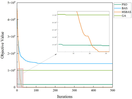
Figure 6.
The comparison of optimization results among four algorithms in the design of altitude compensation module.
After several debugging sessions and appropriate rounding adjustment of the optimal parameters, the following parameter combinations are obtained: is 213 mm, is 25 mm, is 50 mm, the outer angle of connecting rod is , the spring stiffness is 118 N/mm, and the preload value is 27.65 mm, corresponding to the preload force of 3262.7 N. Selecting 0 to 100 mm as the working stroke, the value of the objective function increases to , which meets the design requirements.
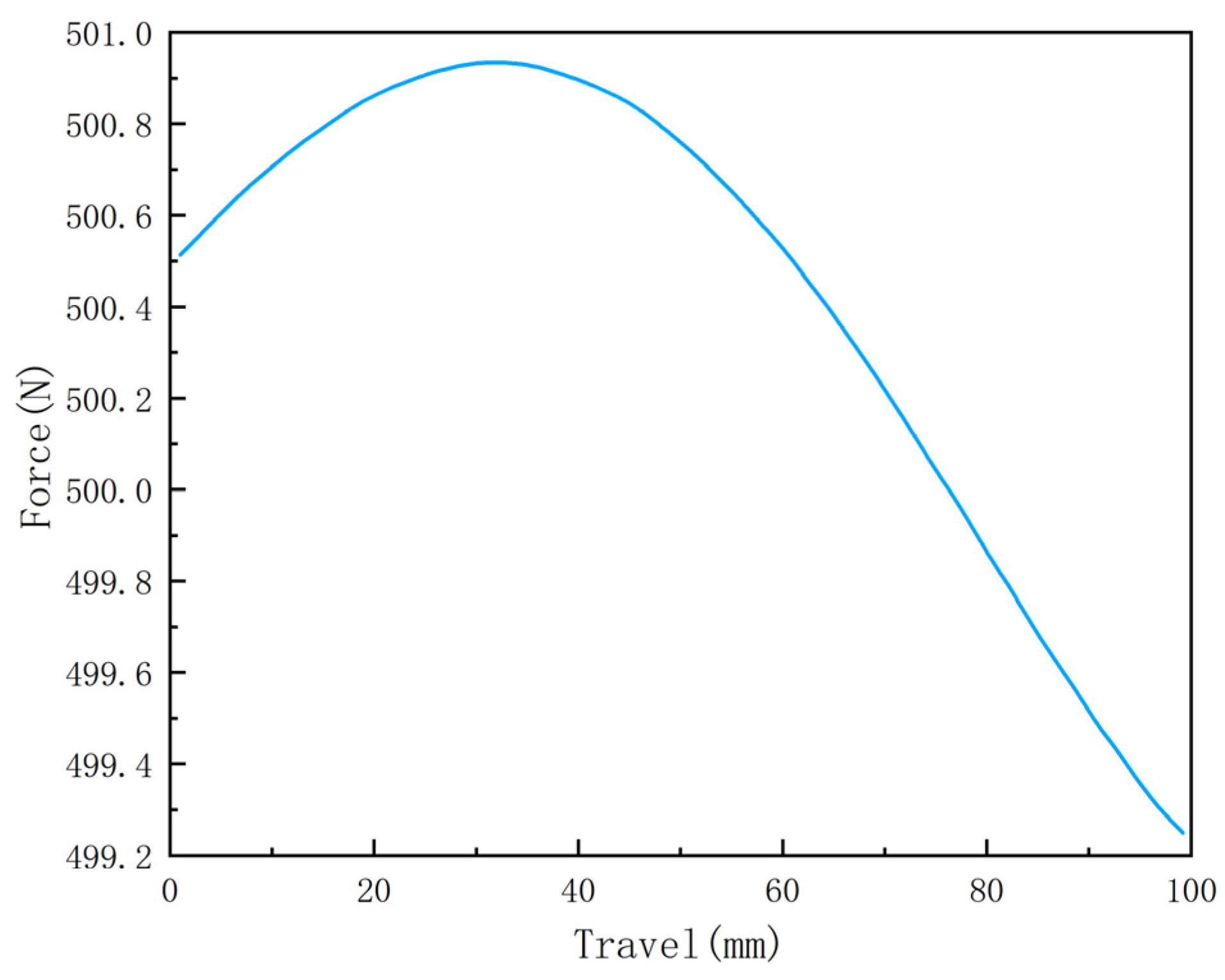
After removing the support force the rod requires, the ideal load curve obtained in different strokes of the height compensation module is shown in Figure 7. With the movement of the rod, the load of the load platform shows a slow rise and then a faster decline in the change trend. The change is mainly located in the rang of 499–501 N, and most of the load is located above 500 N, with a maximum load of 500.92 N and a minimum load of 499.23 N. The maximum deviation of the load is 0.92 N, and the degree of deviation is within 0.25%, which meets the design requirements. The maximum load is 500.92 N, and the minimum load is 499.23 N. The maximum deviation of the load is 0.92 N, and the deviation is within 0.25%, which is in line with the design requirements.
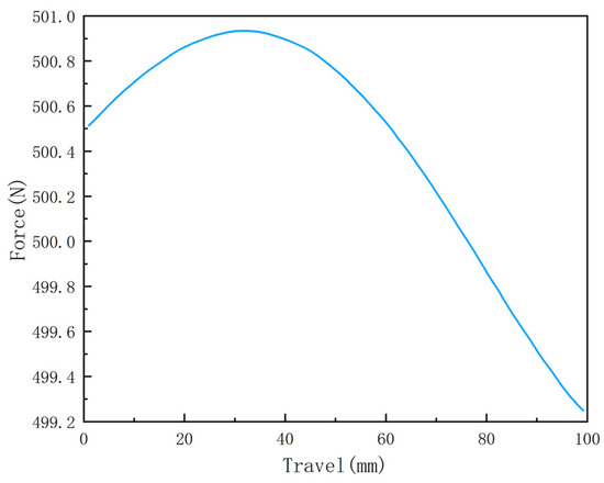
Figure 7.
Curve of load variation with stroke of the altitude compensation module after parameter optimization.
6. Conclusions
This paper adopts a Hybrid Strategy improved Beetle Antennae Search (HSBAS) algorithm to solve the multi-dimensional optimization problem in engineering mechanisms. The HSBAS algorithm introduces three improvement strategies to the BAS algorithm. The adaptive step strategy and multi-directional exploration strategy extend the single search range. The Lens Opposition-Based Learning strategy allows the algorithm to jump out of the local optimum appropriately. It significantly reduces the probability of the algorithm falling into the local optimum and improves the algorithm’s global search ability and stability.
The improved algorithm is tested by the eleven benchmark test functions. HSBAS can reach 1× 10⁻²² accuracy from the optimal value when dealing with low-dimensional functions. It can also obtain 1× 10⁻² accuracy when dealing with high-dimensional functions, significantly improving the algorithm’s capability. According to Friedman’s ranking test result, HSBAS ranks first, which proves that HSBAS effectively avoids the generation of locally optimal solutions and outperforms the optimization capability of the other three algorithm. Regarding convergence performance, HSBAS converges in about 50 steps on low-dimensional functions. On the high-dimensional multi-peak function, due to the need to jump out of the local extreme several times, convergence is performed within 500 steps, which converges slightly slower than other algorithms but has higher precision. HSBAS is further used to optimize the design of the altitude compensation module of the gravity compensation device for solar wings, controlling the fluctuation of bearing capacity within 0.25%, which shows that the algorithm can be used as an effective tool for optimizing engineering problems.
Based on the performance of HSBAS in function optimization, we can conclude that HSBAS has achieved a certain degree of precision in the algorithm’s monolithic exploration. Further improvement can be considered by combining with group strategy or other algorithms, such as the PSO algorithm. The combination of the precision exploration monolithic algorithm and the stochastic multibody parallel exploration PSO algorithm can further expand the search range of the algorithm and improve the solution accuracy, which can be applied in engineering with finer design. It has significant practical value in the field of engineering design applications.
Author Contributions
Conceptualization, S.L. and M.L.; methodology, S.L. and M.L.; validation, S.L., M.L. and X.S.; formal analysis, S.L. and X.S.; investigation, S.L.; resources, X.S., S.L., B.Y. and M.L.; data curation, S.L.; writing—original draft preparation, S.L.; writing—review and editing, S.L., B.Y. and X.S.; visualization, S.L.; supervision, B.Y. and X.S.; project administration, X.S., B.Y.; funding acquisition, X.S., B.Y. All authors have read and agreed to the published version of the manuscript.
Funding
This research received no external funding.
Data Availability Statement
The raw data supporting the conclusions of this article will be made available by the authors on request.
Conflicts of Interest
The authors declare no conflicts of interest.
References
- Kaleka, K.K.; Kaur, A.; Kumar, V. A conceptual comparison of metaheuristic algorithms and applications to engineering design problems. Int. J. Intell. Inf. Database Syst. 2020, 13, 278–306. [Google Scholar] [CrossRef]
- Eesa, A.S.; Hassan, M.M.; Arabo, W.K. Application of optimization algorithms to engineering design problems and discrepancies in mathematical formulas. Appl. Soft Comput. 2023, 140, 110252. [Google Scholar] [CrossRef]
- Yu, L.; Ren, J.; Zhang, J. A Quantum-Based Beetle Swarm Optimization Algorithm for Numerical Optimization. Appl. Sci. 2023, 13, 3179. [Google Scholar] [CrossRef]
- Rajmohan, S.; Elakkiya, E.; Sreeja, S. Multi-cohort whale optimization with search space tightening for engineering optimization problems. Neural Comput. Appl. 2023, 35, 8967–8986. [Google Scholar] [CrossRef]
- Zhang, Y.; Li, S.; Xu, B. Convergence analysis of beetle antennae search algorithm and its applications. Soft Comput. 2021, 25, 10595–10608. [Google Scholar] [CrossRef]
- Liao, L.; Yang, H. Review of Beetle Antennae Search. Comput. Eng. Appl. 2021, 57, 54–64. [Google Scholar] [CrossRef]
- Zhang, J.; Ma, G.; Huang, Y.; Aslani, F.; Nener, B.J. Modelling uniaxial compressive strength of lightweight self-compacting concrete using random forest regression. Constr. Build. Mater. 2019, 210, 713–719. [Google Scholar] [CrossRef]
- Ji, L.; Cao, Z.; Hong, Q.; Chang, X.; Fu, Y.; Shi, J.; Mi, Y.; Li, Z. An improved inverse-time over-current protection method for a microgrid with optimized acceleration and coordination. Energies 2020, 13, 5726. [Google Scholar] [CrossRef]
- Wang, P.; Gao, Y.; Wu, M.; Zhang, F.; Li, G.; Qin, C. A denoising method for fiber optic gyroscope based on variational mode decomposition and beetle swarm antenna search algorithm. Entropy 2020, 22, 765. [Google Scholar] [CrossRef] [PubMed]
- Sun, Y.; Li, G.; Zhang, J. Developing hybrid machine learning models for estimating the unconfined compressive strength of jet grouting composite: A comparative study. Appl. Sci. 2020, 10, 1612. [Google Scholar] [CrossRef]
- Khan, A.H.; Cao, X.; Li, S.; Katsikis, V.N.; Liao, L. BAS-ADAM: An ADAM based approach to improve the performance of beetle antennae search optimizer. IEEE/CAA J. Autom. Sin. 2020, 7, 461–471. [Google Scholar] [CrossRef]
- Wang, J.; Chen, H. BSAS: Beetle swarm antennae search algorithm for optimization problems. arXiv 2018, arXiv:1807.10470. [Google Scholar]
- Li, Q.; Wei, A.; Zhang, Z. Application of economic load distribution of power system based on BAS-PSO. IOP Conf. Ser. Mater. Sci. Eng. 2019, 490, 072056. [Google Scholar] [CrossRef]
- Fan, Q.; Huang, H.; Li, Y.; Han, Z.; Hu, Y.; Huang, D. Beetle antenna strategy based grey wolf optimization. Expert Syst. Appl. 2021, 165, 113882. [Google Scholar] [CrossRef]
- Ye, K.; Shu, L.; Xiao, Z.; Li, W. An improved beetle swarm antennae search algorithm based on multiple operators. Soft Comput. 2024, 1–16. [Google Scholar] [CrossRef]
- Zhao, Q.; Zheng, Z.J. Computational and Mathematical Methods in Medicine Prediction of COVID-19 in BRICS Countries: An Integrated Deep Learning Model of CEEMDAN-R-ILSTM-Elman. Comput. Math. Methods Med. 2022, 2022, 1566727. [Google Scholar] [CrossRef] [PubMed]
- Liao, L.; Ouyang, Z. Beetle antennae search based on quadratic interpolation. Appl. Res. Comput. 2021, 38, 745–750. [Google Scholar] [CrossRef]
- Zhu, Z.; Zhang, Z.; Man, W.; Tong, X.; Qiu, J.; Li, F. A new beetle antennae search algorithm for multi-objective energy management in microgrid. In Proceedings of the 2018 13th IEEE Conference on Industrial Electronics and Applications (ICIEA), Wuhan, China, 31 May–2 June 2018; IEEE: Piscataway, NJ, USA, 2018; pp. 1599–1603. [Google Scholar]
- Xie, S.; Chu, X.; Zheng, M.; Liu, C. Ship predictive collision avoidance method based on an improved beetle antennae search algorithm. Ocean Eng. 2019, 192, 106542. [Google Scholar] [CrossRef]
- Li, X.; Jiang, H.; Niu, M.; Wang, R. An enhanced selective ensemble deep learning method for rolling bearing fault diagnosis with beetle antennae search algorithm. Mech. Syst. Signal Process. 2020, 142, 106752. [Google Scholar] [CrossRef]
- Zhang, J.; Sun, Y.; Li, G.; Wang, Y.; Sun, J.; Li, J. Machine-learning-assisted shear strength prediction of reinforced concrete beams with and without stirrups. Eng. Comput. 2022, 38, 1293–1307. [Google Scholar] [CrossRef]
- Khan, A.H.; Li, S.; Luo, X. Obstacle Avoidance and Tracking Control of Redundant Robotic Manipulator: An RNN based Metaheuristic Approach. IEEE Trans. Ind. Inform. 2020, 16, 4670–4680. [Google Scholar] [CrossRef]
- Wang, Y.; Chen, Z.; Zu, H.; Zhang, X. An optimized RBF neural network based on beetle antennae search algorithm for modeling the static friction in a robotic manipulator joint. Math. Probl. Eng. 2020, 2020, 5839195. [Google Scholar] [CrossRef]
- Bullnheimer, B. A new rank based version of the ant system: A computational study. Cent. Eur. J. Oper. Res. Econ 1999, 7, 25–38. [Google Scholar]
- Jiang, X.; Li, S.J. BAS: Beetle antennae search algorithm for optimization problems. arXiv 2017, arXiv:1710.10724. [Google Scholar] [CrossRef]
- Rahnamayan, S.; Tizhoosh, H.R.; Salama, M.M. Opposition versus randomness in soft computing techniques. Appl. Soft Comput. 2008, 8, 906–918. [Google Scholar] [CrossRef]
- Yue, Y.; Zhou, Y.; Xu, L.; Zhao, D. Optimal Defense Strategy Selection Algorithm Based on Reinforcement Learning and Opposition-Based Learning. Appl. Sci. 2022, 12, 9594. [Google Scholar] [CrossRef]
- Long, W.; Wu, T.-B.; Tang, M.-Z.; Xu, M.; Ca, S.-H. Grey wolf optimizer algorithm based on lens imaging learning strategy. Acta Autom. Sin. 2020, 46, 2148–2164. [Google Scholar] [CrossRef]
- Xu, J.; Xu, S.; Zhang, L.; Zhou, C.; Han, Z. A particle swarm optimization algorithm based on diversity-driven fusion of opposing phase selection strategies. Complex Intell. Syst. 2023, 9, 6611–6643. [Google Scholar] [CrossRef]
- Wang, Z.; Ding, H.; Wang, J.; Li, B.; Hou, P.; Yang, Z. Salp swarm algorithm based on orthogonal refracted opposition-based learning. J. Harbin Inst. Technol. 2022, 54, 122–136. [Google Scholar]


Disclaimer/Publisher’s Note: The statements, opinions and data contained in all publications are solely those of the individual author(s) and contributor(s) and not of MDPI and/or the editor(s). MDPI and/or the editor(s) disclaim responsibility for any injury to people or property resulting from any ideas, methods, instructions or products referred to in the content. |
© 2024 by the authors. Licensee MDPI, Basel, Switzerland. This article is an open access article distributed under the terms and conditions of the Creative Commons Attribution (CC BY) license (https://creativecommons.org/licenses/by/4.0/).