Bearing Fault Diagnosis Based on Parameter-Optimized Variational Mode Extraction and an Improved One-Dimensional Convolutional Neural Network

Abstract

When faults occur in rolling bearings, vibration signals exhibit sensitivity to periodic impact components, susceptibility to complex background noise, and non-stationary and nonlinear characteristics. Consequently, using traditional signal processing methods to effectively identify bearing faults presents significant challenges. To facilitate the accurate fault diagnosis of bearings in noisy conditions, we propose an intelligent fault diagnosis method using the Archimedes optimization algorithm (AOA), coupled with a one-dimensional multi-scale residual convolutional neural network (1D-MRCNN), to optimize the variational mode extraction (VME) parameters. First, we introduce a weighted correlated kurtosis (WCK) indicator, formulated using the correlation coefficient and correlated kurtosis as the objective function, to optimize the VME’s center frequency ω and penalty factor α, enabling targeted signal extraction. Second, deep learning techniques are employed to construct the 1D-MRCNN. The neural network then processes the extracted signal for feature extraction and automated fault-type identification. Our simulation results show that the WCK objective function effectively isolates impact components under fault conditions, and our experimental validation confirms that the proposed method accurately identifies diverse fault types across multiple noise levels.

1. Introduction

Rolling bearings are integral components of high-speed and high-power systems, and are prone to failure due to fatigue, wear, excessive loads, and other factors. Among the variety of bearings available, ceramic bearings are distinguished by their exceptional performance in high-speed environments, which is attributed to their low density, high hardness, resistance to wear, and thermal expansion. These characteristics not only reduce energy loss due to friction, but also enhance the longevity of machinery components, making ceramic bearings an ideal choice for a plethora of advanced engineering applications. Therefore, accurate fault diagnosis is essential to prevent undue operational interruptions and minimize economic losses [1]. Shi et al. [2] introduced a discrete-time model for ceramic bearings considering incipient faults, and proposed a modified observer with enhanced design freedom compared to traditional Luenberger observers. Gao et al. [3] developed an ultra-high-speed hybrid ceramic rolling element triboelectric bearing to enable the real-time monitoring of dynamic behavior and stability. Industrial failures typically manifest as weak periodic shocks in bearing signals, exhibiting non-stationary and nonlinear characteristics that can be obscured by background noise [4]. Therefore, signal processing techniques are crucial for noise reduction in vibration signals. Techniques like empirical mode decomposition (EMD) [5], ensemble empirical mode decomposition (EEMD) [6,7], wavelet threshold denoising (WTD) [8], and local mean decomposition (LMD) [9] have been applied for noise elimination in vibration signals, proving their efficacy in signal processing. However, EMD and LMD struggle with issues like mode mixing and endpoint effects, while EEMD, although it addresses mode mixing by introducing white noise to each decomposition, does not entirely resolve mode mixing and endpoint challenges. WTD’s noise reduction success is highly dependent on the threshold value selection. VMD [10] emerges as a non-recursive, adaptive technique that decomposes signals into specific frequency-centered modes with finite bandwidths, overcoming the limitations of EMD and related methods. Jiang et al. [11] enhanced VMD’s efficacy in diagnosing bearing faults by adaptively determining the signal modes and optimizing the initial center frequencies. Wang et al. [12] explored VMD’s equivalent filtering characteristics and applied their insights to diagnose faults in rotors and stators. Li et al. [13] advanced the application of VMD by integrating it with a kernel extreme learning machine for enhanced fault diagnosis in rolling bearings. However, VMD’s effectiveness is heavily dependent on certain parameters, such as the number of decomposition layers K and the penalty factor α [14,15]. As demonstrated above, there is a considerable amount of research on parameter-optimized VMD [16,17,18]. Incorrect settings can result in over or under decomposition, highlighting the importance of selecting suitable objective functions and optimizing the parameters for reliable results. The key objective functions in this domain include envelope entropy [19], ensemble kurtosis [20], and envelope spectrum kurtosis [21], which, despite their decomposition efficacy, are sensitive to noise. Correlated kurtosis (CK) [22,23], which considers the periodicity of bearing fault signals and effectively isolates non-periodic components, represents a potential solution to this problem. Additionally, the correlation coefficient offers insights into signal similarities [24]. Leveraging the strengths of correlated kurtosis and the correlation coefficient, weighted correlated kurtosis (WCK) has been devised as a comprehensive objective function. However, VMD’s computational demands and sensitivity to mode count underscore the importance of careful parameter selection and optimization to ensure accurate and reliable fault diagnosis outcomes.

To address the challenges posed by VMD, Nazari et al. [25] proposed variational mode extraction (VME), an approach derived from VMD. By accurately determining the center frequency ω and penalty factor α, VME efficiently isolates the desired mode components, significantly reducing the computation time. This method has been effectively applied to fault diagnosis of rolling bearings. Ye et al. [26] combined VME with an improved one-dimensional convolutional neural network for the intelligent diagnosis of rolling bearings. However, the selection of the VME parameters was based on empirical judgment, raising concerns about its reliability. Yan et al. [27] employed the whale optimization algorithm to refine the parameters of VME, integrating this improved algorithm with the k-nearest neighbor algorithm (KNN). Liu et al. [28] proposed a window fusion strategy that adaptively determines the center frequency ω and penalty factor α. Despite this innovation, their method still necessitates manual intervention for fault identification, highlighting a gap in the development of fully automated, intelligent diagnostic systems.

In recent years, intelligent fault diagnosis has emerged as a novel and increasingly popular approach. Common methodologies in this domain include the back-propagation neural network (BPNN), support vector machine (SVM), and random forest (RF). These techniques are adept at determining the health status of bearings through effective feature selection and extraction. However, the manual process of feature extraction remains time consuming. Identifying features that are highly sensitive to vibration signals and filtering out noise remain significant challenges. Deep learning, a subset of machine learning, has attracted research interest in recent years, especially with the advancements in computational capabilities and sensor technology [29]. Saucedo-Dorantes et al. [30] used stacked autoencoder structures for feature extraction and fusion to achieve an enhanced condition assessment, demonstrating its effectiveness for fault diagnosis across various bearing technologies. The convolutional neural network (CNN) [31,32], primarily recognized for its applications in image processing, leverages a local receptive field, shared weights, and subsampling within a spatial domain. This approach significantly reduces the computational demands on the network, minimizes the risk of overfitting, and facilitates the automatic extraction of crucial signal features [33]. CNNs are typically employed for pattern recognition using two approaches: directly using the vibration signal as the input and preprocessing the vibration signal into a two-dimensional image for model input. The latter often involves transforming the vibration signal into a grayscale image [34,35], or converting it into a time-domain image through continuous wavelet transform or short-time Fourier transform [36,37,38,39]. Despite the success of two-dimensional CNNs in intelligent fault diagnosis [40,41], vibration signals are inherently one-dimensional sequences. Converting them into two-dimensional images necessitates extra preprocessing, potentially exaggerating the impact of periodic shock signals and reducing diagnostic efficacy in noisy conditions. Consequently, some scholars have explored directly using one-dimensional vibration signals as inputs for diagnosis via a 1D-CNN. For example, Wang et al. [42] employed vibration and acoustic signals as inputs for a 1D-CNN in their diagnostic models; Habbouche et al. [43] utilized VMD-preprocessed vibration signals with a 1D-CNN for diagnosis; and Shao et al. [44] applied a 1D-CNN for fault feature extraction and trained an SVM on rolling bearing fault diagnosis. However, traditional 1D-CNNs face the challenges of computational demand and limited noise immunity. To overcome these issues, this study proposes a one-dimensional multi-scale residual convolutional neural network (1D-MRCNN), designed to lower the computational costs and enhance noise resistance.

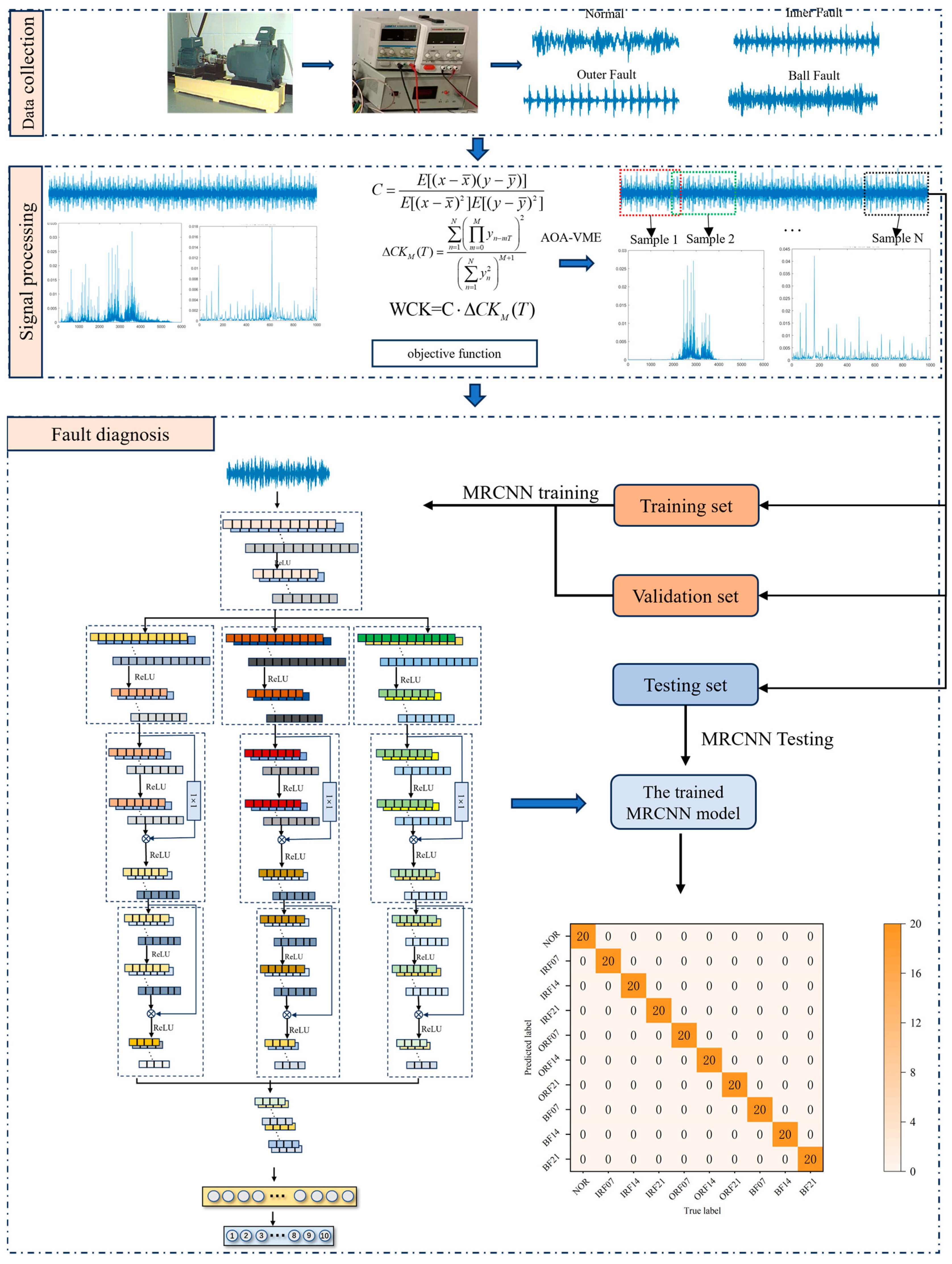
In summary, we propose a rolling bearing intelligent diagnosis scheme based on the Archimedes optimization algorithm (AOA), to optimize the parameters of VME and a 1D-MRCNN. Initially, WCK serves as the objective function to optimize the penalty factor α and center frequency ω of the VME, aiming to extract the desired mode components and eliminate noise in the vibration signals. Then, the processed vibration signals are input into the 1D-MRCNN for fault diagnosis. The fusion of VME with the 1D-MRCNN maximizes the advantages of both techniques, thereby enhancing recognition accuracy.

The following is an overview of this paper: Section 2 presents related works (pertaining to AOA, VME, and 1D-MRCNN); Section 3 employs simulated signals to validate the feasibility of parameter-optimized VME using WCK as the objective function; in Section 4, the experimental signals are analyzed and compared to demonstrate the practicality and superiority of the proposed method; and Section 5 presents our conclusions.

2. Related Works

2.1. Variational Mode Extraction

The VME algorithm is derived from VMD and shares a similar mathematical principle. However, VME extracts a single specific component, resulting in higher efficiency. In VME, the input signal $\mathrm{s}(\mathrm{t})$ is decomposed into two parts:

$$\mathrm{s}(\mathrm{t}){=\mathrm{u}}_{\mathrm{d}}(\mathrm{t})+{\mathrm{s}}_{\mathrm{r}}(\mathrm{t})$$

(1)

In Equation (1), ${\mathrm{u}}_{\mathrm{d}}(\mathrm{t})$ represents the desired mode component, and ${\mathrm{s}}_{\mathrm{r}}(\mathrm{t})$ represents the residual signal.

Moreover, ${\mathrm{u}}_{\mathrm{d}}(\mathrm{t})$ needs to be compactly surrounded by the center frequency ω after the Hilbert transform and have minimal overlap with ${\mathrm{u}}_{\mathrm{d}}(\mathrm{t})$ and ${\mathrm{s}}_{\mathrm{r}}(\mathrm{t})$. Therefore, the constraints need to be minimized to obtain the desired mode components, as follows:

$${\mathrm{J}}_1={‖{\partial }_{\mathrm{t}}\left[\left(\mathsf{\delta }(\mathrm{t})+\frac{\mathrm{j}}{\mathsf{\pi }\mathrm{t}}\right)\ast {\mathrm{u}}_{\mathrm{d}}(\mathrm{t})\right]{\mathrm{e}}^{-\mathrm{j}{\mathsf{\omega }}_{\mathrm{d}}\mathrm{t}}‖}_2^2$$

(2)

In Equation (2), $\mathsf{\delta }$ represents the Dirac distribution, ${\mathsf{\omega }}_{\mathrm{d}}$ denotes the center frequency of the mode component ${\mathrm{u}}_{\mathrm{d}}(\mathrm{t})$, and ∗ denotes the convolution operation.

The spectral overlap between ${\mathrm{u}}_{\mathrm{d}}(\mathrm{t})$ and ${\mathrm{s}}_{\mathrm{r}}(\mathrm{t})$ is minimized, and a penalty function is introduced, as follows:

$${\mathrm{J}}_2=\parallel \mathsf{\beta }(\mathrm{t})\ast {\mathrm{s}}_{\mathrm{r}}(\mathrm{t}){\parallel }_2^2$$

(3)

In Equation (3), $\mathsf{\beta }(\mathrm{t})$ represents the impulse response of the frequency response filter.

Therefore, the problem of finding modes can be formulated as a problem of constrained minimization when Equations (2) and (3) are combined:

$$\begin{array}{l}{\min }_{{\mathrm{u}}_{\mathrm{d}},{\mathsf{\omega }}_{\mathrm{d}},{\mathrm{s}}_{\mathrm{r}}}\{\mathsf{\alpha }{\mathrm{J}}_1+{\mathrm{J}}_2\}\\ \mathrm{s}\mathrm{u}\mathrm{b}\mathrm{j}\mathrm{e}\mathrm{c}\mathrm{t}\hspace{0.17em}\mathrm{t}\mathrm{o}:{\mathrm{u}}_{\mathrm{d}}(\mathrm{t})+{\mathrm{s}}_{\mathrm{r}}(\mathrm{t})=\mathrm{s}(\mathrm{t})\end{array}$$

(4)

In Equation (4), $\mathsf{\alpha }$ denotes the parameter that balances ${\mathrm{J}}_1$ and ${\mathrm{J}}_2$.

The previously described constrained optimization problem is transformed into an unconstrained format. This involves incorporating both a quadratic penalty term and Lagrange multipliers $\mathsf{\lambda }$, thereby forming the augmented Lagrange function:

$$\begin{array}{l}\mathsf{\Gamma }({\mathrm{u}}_{\mathrm{d}},{\mathsf{\omega }}_{\mathrm{d}},\mathsf{\lambda })=\mathsf{\alpha }\Vert \mathrm{j}(\mathsf{\omega }-{\mathsf{\omega }}_{\mathrm{d}})[1+\mathrm{sgn}(\mathsf{\omega }){\widehat{\mathrm{u}}}_{\mathrm{d}}]{\Vert }_2^2+\Vert \widehat{\mathsf{\beta }}(\mathsf{\omega })\ast {\widehat{\mathrm{f}}}_{\mathrm{r}}(\mathsf{\omega }){\Vert }_2^2\\ +\Vert \widehat{\mathrm{f}}(\mathsf{\omega })-({\widehat{\mathrm{u}}}_{\mathrm{d}}(\mathsf{\omega })+{\widehat{\mathrm{f}}}_{\mathrm{r}}(\mathsf{\omega })){\Vert }_2^2+\langle \widehat{\mathsf{\lambda }}(\mathsf{\omega }),\widehat{\mathrm{f}}(\mathsf{\omega })-({\widehat{\mathrm{u}}}_{\mathrm{d}}(\mathsf{\omega })+{\widehat{\mathrm{f}}}_{\mathrm{r}}(\mathsf{\omega }))\rangle \end{array}$$

(5)

The alternating direction method of multipliers is used to find the saddle point of the Lagrange function.

The steps are as follows:

• Initialize ${\widehat{\mathsf{\mu }}}_{\mathrm{d}}^1$, ${\widehat{\mathsf{\lambda }}}^1$, ${\widehat{\mathsf{\omega }}}_{\mathrm{d}}^1$, n = 1, and estimate the initial value of ${\widehat{\mathsf{\omega }}}_{\mathrm{d}}^1$.
• According to Equation (6), update ${\widehat{\mathsf{\mu }}}_{\mathrm{d}}$:

  $${\widehat{\mathrm{u}}}_{\mathrm{d}}^{\mathrm{n}+1}(\mathsf{\omega })=\frac{\widehat{\mathrm{x}}(\mathsf{\omega })+{\mathsf{\alpha }}^2{(\mathsf{\omega }-{\mathsf{\omega }}_{\mathrm{d}}^{\mathrm{n}+1})}^4\cdot {\widehat{\mathrm{u}}}_{\mathrm{d}}^{\mathrm{n}}(\mathsf{\omega })+\widehat{\mathsf{\lambda }}(\mathsf{\omega })/2}{\left[1+{\mathsf{\alpha }}^2{(\mathsf{\omega }-{\mathsf{\omega }}_{\mathrm{d}}^{\mathrm{n}+1})}^4\right]\left[1+2\mathsf{\alpha }{(\mathsf{\omega }-{\mathsf{\omega }}_{\mathrm{d}}^{\mathrm{n}})}^2\right]}$$

  (6)
• According to Equation (7), update ${\mathsf{\omega }}_{\mathrm{d}}$:

  $${\mathsf{\omega }}_{\mathrm{d}}^{\mathrm{n}+1}=\frac{{\displaystyle {\int }_0^{\infty }\mathsf{\omega }}{\left|{\mathrm{u}}_{\mathrm{d}}^{\mathrm{n}+1}(\mathsf{\omega })\right|}^2\mathrm{d}\mathsf{\omega }}{{\displaystyle {\int }_0^{\infty }{\left|{\mathrm{u}}_{\mathrm{d}}^{\mathrm{n}+1}(\mathsf{\omega })\right|}^2}\mathrm{d}\mathsf{\omega }}$$

  (7)
• According to Equation (8), update the Lagrange multipliers for all ω > 0:

  $${\widehat{\mathsf{\lambda }}}^{\mathrm{n}+1}={\widehat{\mathsf{\lambda }}}^{\mathrm{n}}+\mathsf{\tau }\cdot \left[\frac{\widehat{\mathrm{x}}(\mathsf{\omega })-{\widehat{\mathrm{u}}}_{\mathrm{d}}^{\mathrm{n}+1}(\mathsf{\omega })}{1+{\mathsf{\alpha }}^2{(\mathsf{\omega }-{\mathsf{\omega }}_{\mathrm{d}}^{\mathrm{n}+1})}^4}\right]$$

  (8)
• Repeat steps 2~4 until the iteration stop condition is satisfied:

  $$\frac{{‖{\widehat{\mathrm{u}}}_{\mathrm{d}}^{\mathrm{n}+1}-{\widehat{\mathrm{u}}}_{\mathrm{d}}^{\mathrm{n}}‖}_2^2}{{‖{\widehat{\mathrm{u}}}_{\mathrm{d}}^{\mathrm{n}}‖}_2^2}<\mathsf{\epsilon }$$

  (9)
• End the loop and obtain the desired mode ${\mathrm{u}}_{\mathrm{d}}(\mathrm{t})$.

2.2. Archimedes Optimization Algorithm for Optimizing VME

2.2.1. Weighted Correlated Kurtosis

In VME, the objective function chosen for optimizing the center frequency ω and penalty factor α is correlated kurtosis, which is particularly sensitive to periodic impact components. The function for correlated kurtosis is as follows:

$$\mathsf{\Delta }\mathrm{C}{\mathrm{K}}_{\mathrm{M}}(\mathrm{T})=\frac{{\displaystyle \sum _{\mathrm{n}=1}^{\mathrm{N}}{\left({\displaystyle \prod _{\mathrm{m}=0}^{\mathrm{M}}{\mathrm{y}}_{\mathrm{n}-\mathrm{m}\mathrm{T}}}\right)}^2}}{{\left({\displaystyle \sum _{\mathrm{n}=1}^{\mathrm{N}}{\mathrm{y}}_{\mathrm{n}}^2}\right)}^{\mathrm{M}+1}}$$

(10)

In Equation (10), M represents the shift, and T represents the impact signal period.

When T = 0 and M = 1, correlated kurtosis is equivalent to kurtosis. The superiority of correlated kurtosis lies in its heightened sensitivity to periodic impacts, making it more effective for extracting fault features in rotating machinery, such as rolling bearings.

The correlation coefficient, which quantifies the similarity between two signals, facilitates the detection of maximum similarity between the original and decomposed signals. This process aims to retain as much useful information as possible. The expression of the correlation coefficient is shown as follows:

$$\mathrm{C}=\frac{\mathrm{E}[(\mathrm{x}-\overline{\mathrm{x}})(\mathrm{y}-\overline{\mathrm{y}})]}{\mathrm{E}[{(\mathrm{x}-\overline{\mathrm{x}})}^2]\mathrm{E}[{(\mathrm{y}-\overline{\mathrm{y}})}^2]}$$

(11)

In Equation (11), $\mathrm{E}[\cdot ]$ represents the mathematical expectation, and C represents the correlation coefficient between signals x and y.

However, the correlation coefficient is susceptible to noise interference. Therefore, this paper takes into account the distinct advantages of both correlated kurtosis and the correlation coefficient. With these considerations, WCK is utilized as the objective function for parameter-optimized VME. The expression of WCK is shown as follows:

$$\mathrm{WCK}=\mathrm{C}\cdot \mathsf{\Delta }\mathrm{C}{\mathrm{K}}_{\mathrm{M}}(\mathrm{T})$$

(12)

2.2.2. Archimedes Optimization Algorithm

The AOA, a new heuristic algorithm proposed by Hashim et al. [45], is designed for complex problems prone to local optimal solutions. In this algorithm, each individual is represented as an immersed object, and its acceleration is updated based on collisions with neighboring objects. The individual’s new position is determined by considering factors such as density, volume, and acceleration.

The initial location of an individual is defined as follows:

$${\mathrm{O}}_{\mathrm{i}}=\mathrm{l}{\mathrm{b}}_{\mathrm{i}}+\mathrm{r}\times (\mathrm{u}{\mathrm{b}}_{\mathrm{i}}-\mathrm{l}{\mathrm{b}}_{\mathrm{i}})$$

(13)

In Equation (13), $\mathrm{l}{\mathrm{b}}_{\mathrm{i}}$ and $\mathrm{u}{\mathrm{b}}_{\mathrm{i}}$ denote the lower and upper bounds of the search range, and $\mathrm{r}$ denotes a random number in the range [0,1].

Acceleration, density, and volume are initialized as follows:

$$\left\{\begin{array}{l}\mathrm{a}\mathrm{c}{\mathrm{c}}_{\mathrm{i}}=\mathrm{l}{\mathrm{b}}_{\mathrm{i}}+\mathrm{r}\times \left(\mathrm{u}{\mathrm{b}}_{\mathrm{i}}-\mathrm{l}{\mathrm{b}}_{\mathrm{i}}\right)\hfill \\ \mathrm{d}\mathrm{e}{\mathrm{n}}_{\mathrm{i}}=\mathrm{r}\hfill \\ \mathrm{v}\mathrm{o}{\mathrm{l}}_{\mathrm{i}}=\mathrm{r}\hfill \end{array}\right.$$

(14)

In this step, the initial population is evaluated, and the individual with the best fitness is selected and assigned $\mathrm{a}\mathrm{c}{\mathrm{c}}_{\mathrm{b}\mathrm{e}\mathrm{s}\mathrm{t}}$, $\mathrm{d}\mathrm{e}{\mathrm{n}}_{\mathrm{b}\mathrm{e}\mathrm{s}\mathrm{t}}$, and $\mathrm{v}\mathrm{o}{\mathrm{l}}_{\mathrm{b}\mathrm{e}\mathrm{s}\mathrm{t}}$.

The updated density and volume are as follows:

$$\left\{\begin{array}{l}{\mathrm{den}}_{\mathrm{i}}^{\mathrm{t}+1}={\mathrm{den}}_{\mathrm{i}}^{\mathrm{t}}+\mathrm{r}\times \left({\mathrm{den}}_{\mathrm{best}}-{\mathrm{den}}_{\mathrm{i}}^{\mathrm{t}}\right)\hfill \\ {\mathrm{vol}}_{\mathrm{i}}^{\mathrm{t}+1}={\mathrm{vol}}_{\mathrm{i}}^{\mathrm{t}}+\mathrm{r}\times \left({\mathrm{vol}}_{\mathrm{best}}-{\mathrm{vol}}_{\mathrm{i}}^{\mathrm{t}}\right)\hfill \end{array}\right.$$

(15)

In Equation (15), $\mathrm{t}$ represents the current iteration, $\mathrm{d}\mathrm{e}{\mathrm{n}}_{\mathrm{b}\mathrm{e}\mathrm{s}\mathrm{t}}$ and $\mathrm{v}\mathrm{o}{\mathrm{l}}_{\mathrm{b}\mathrm{e}\mathrm{s}\mathrm{t}}$ represent the best individual density and volume found so far, and $\mathrm{a}\mathrm{c}{\mathrm{c}}_{\mathrm{b}\mathrm{e}\mathrm{s}\mathrm{t}}$ denotes the current individual optimal acceleration.

The transition from collision to balance between individuals is controlled by the balance factor TF. This signifies the transition from the exploration phase to the exploitation phase, as follows:

$$\mathrm{T}\mathrm{F}=\exp \left(\frac{\mathrm{t}-{\mathrm{t}}_{\max }}{{\mathrm{t}}_{\max }}\right)$$

(16)

In Equation (16), ${\mathrm{t}}_{\max }$ represents the maximum number of iterations.

The density factor $\mathrm{d}$ determines the position state of the individual, which helps the AOA search from global to local optima:

$${\mathrm{d}}^{\mathrm{t}+1}=\exp (\frac{{\mathrm{t}}_{\mathrm{m}\mathrm{a}\mathrm{x}}-\mathrm{t}}{{\mathrm{t}}_{\mathrm{m}\mathrm{a}\mathrm{x}}})-(\frac{\mathrm{t}}{{\mathrm{t}}_{\mathrm{m}\mathrm{a}\mathrm{x}}})$$

(17)

The individual acceleration at iteration $\mathrm{t}+1$ is updated as follows:

$$\left\{\begin{array}{ll}{\mathrm{acc}}_{\mathrm{i}}^{\mathrm{t}+1}=\frac{{\mathrm{den}}_{\mathrm{mr}}+{\mathrm{vol}}_{\mathrm{mr}}\times {\mathrm{acc}}_{\mathrm{mr}}}{{\mathrm{den}}_{\mathrm{i}}^{\mathrm{t}+1}\times {\mathrm{vol}}_{\mathrm{i}}^{\mathrm{t}+1}}\hfill & \mathrm{T}\mathrm{F}\le 0.5\hfill \\ {\mathrm{acc}}_{\mathrm{i}}^{\mathrm{t}+1}=\frac{{\mathrm{den}}_{\mathrm{best}}+{\mathrm{vol}}_{\mathrm{best}}\times {\mathrm{acc}}_{\mathrm{best}}}{{\mathrm{den}}_{\mathrm{i}}^{\mathrm{t}+1}\times {\mathrm{vol}}_{\mathrm{i}}^{\mathrm{t}+1}}\hfill & \mathrm{T}\mathrm{F}>0.5\hfill \end{array}\right.$$

(18)

In Equation (18), ${\mathrm{den}}_{\mathrm{mr}}$, ${\mathrm{vol}}_{\mathrm{mr}}$, and ${\mathrm{acc}}_{\mathrm{mr}}$, denote the density, volume, and acceleration, respectively, of a random individual.

Acceleration within the algorithm is normalized to facilitate optimal search behavior. When the target is distant from the global optimum, the acceleration is set at a high value, indicative of the exploration stage. Conversely, when the target nears the global optimum, the acceleration is reduced, signifying the transition to the exploitation stage:

$${\mathrm{acc}}_{\mathrm{i}-\mathrm{norn}}^{\mathrm{t}+1}=\mathrm{u}\times \frac{{\mathrm{acc}}_1^{\mathrm{t}+1}-\min (\mathrm{acc})}{\max (\mathrm{acc})-\min (\mathrm{acc})}+1$$

(19)

In Equation (19), $\mathrm{u}$ and $\mathrm{l}$ are the standardization parameters and are set to 0.9 and 0.1, respectively.

The individual position at iteration $\mathrm{t}+1$ is updated as follows:

$$\left\{\begin{array}{ll}{\mathrm{x}}_{\mathrm{i}}^{\mathrm{t}+1}={\mathrm{x}}_{\mathrm{i}}^{\mathrm{t}}+{\mathrm{C}}_1\times \mathrm{r}\times \mathrm{a}\mathrm{c}{\mathrm{c}}_{\mathrm{i}-\mathrm{n}\mathrm{o}\mathrm{r}\mathrm{m}}^{\mathrm{t}+1}\times \mathrm{d}\times \left({\mathrm{x}}_{\mathrm{r}}-{\mathrm{x}}_{\mathrm{i}}^{\mathrm{t}}\right)\hfill & \mathrm{T}\mathrm{F}\le 0.5\hfill \\ {\mathrm{x}}_{\mathrm{i}}^{\mathrm{t}+1}={\mathrm{x}}_{\mathrm{b}\mathrm{e}\mathrm{s}\mathrm{t}}^{\mathrm{t}}+\mathrm{F}\times {\mathrm{C}}_2\times \mathrm{r}\times \mathrm{a}\mathrm{c}{\mathrm{c}}_{\mathrm{i}-\mathrm{n}\mathrm{o}\mathrm{r}\mathrm{m}}^{\mathrm{t}+1}\times \mathrm{d}\times \left(\mathrm{T}\times {\mathrm{x}}_{\mathrm{b}\mathrm{e}\mathrm{s}\mathrm{t}}-{\mathrm{x}}_{\mathrm{i}}^{\mathrm{t}}\right)\hfill & \mathrm{T}\mathrm{F}>0.5\hfill \end{array}\right.$$

(20)

In Equation (20), ${\mathrm{C}}_1$ is set at 2, ${\mathrm{C}}_2$ is set at 6, $\mathrm{T}$ increases with the number of iterations in the range $[0{.3\mathrm{C}}_2,1]$, and $\mathrm{F}$, which represents the direction factor, is defined as follows:

$$\mathrm{F}=\left\{\begin{array}{ll}+1\hfill & \hspace{1em}\hspace{1em}\hspace{1em}\mathrm{P}\le 0.5\hfill \\ -1\hfill & \hspace{1em}\hspace{1em}\mathrm{P}>0.5\hfill \end{array}\right.$$

(21)

In Equation (21), $\mathrm{P}=2\times \mathrm{r}-{\mathrm{C}}_4$, ${\mathrm{C}}_4$ is set at 0.5.

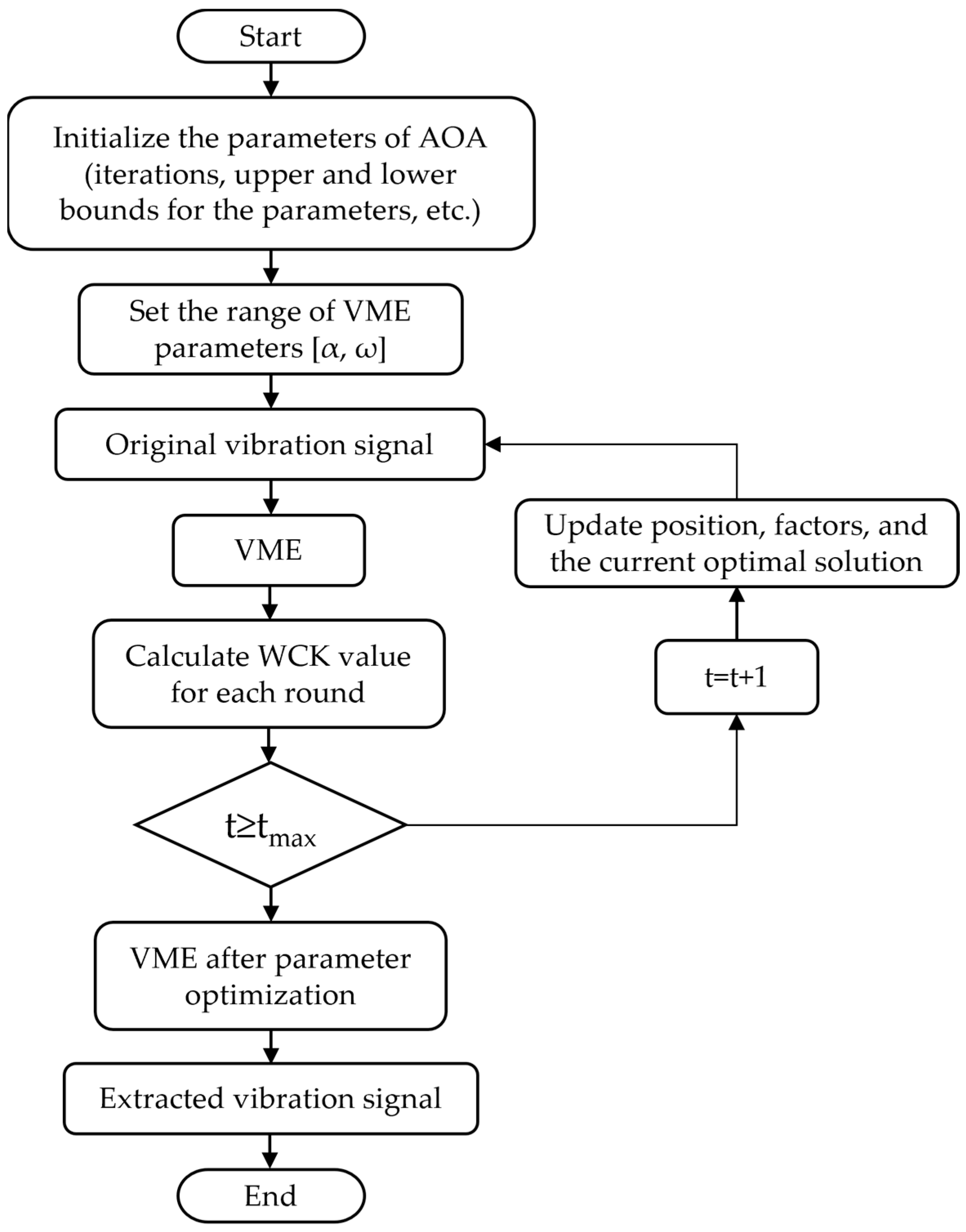
A flowchart of the process for optimizing the parameters of VME using the AOA is shown in Figure 1.

2.3. One-Dimensional Convolutional Neural Network

The convolutional neural network, a prominent deep learning algorithm, possesses exceptional feature learning capabilities. Due to its significant breakthroughs in image processing, it has garnered attention from scholars with regard to its potential in fault diagnosis applications.

A standard one-dimensional CNN consists of four key components: a convolutional layer, a pooling layer, a fully connected layer, and a classification layer.

Within the convolutional layer, the input signal undergoes convolution using a convolutional kernel at a specified step size:

$${\mathrm{y}}_{\mathrm{i}}^{\mathrm{l}}=\mathrm{f}({\displaystyle \sum _{\mathrm{j}=0}^{\mathrm{k}-1}{\mathrm{w}}_{\mathrm{j}}^{\mathrm{l}}}\cdot {\mathrm{x}}_{\mathrm{i}+\mathrm{j}}^{\mathrm{l}-1}+{\mathrm{b}}_{\mathrm{i}}^{\mathrm{l}})$$

(22)

In Equation (22), ${\mathrm{y}}_{\mathrm{i}}^{\mathrm{l}}$ represents the output value of the $\mathrm{i}$th neuron in the $\mathrm{i}$th convolutional layer, $\mathrm{f}(·)$ represents the activation function, ${\mathrm{w}}_{\mathrm{j}}^{\mathrm{l}}$ represents the weight parameter of the $\mathrm{j}$th convolution kernel in the $\mathrm{l}$th layer, ${\mathrm{x}}_{\mathrm{i}+\mathrm{j}}^{\mathrm{l}-1}$ represents the $\mathrm{i}$th input value of the $\mathrm{l}-1$ layer input in the $\mathrm{j}$th convolution kernel, ${\mathrm{b}}_{\mathrm{i}}^{\mathrm{l}}$ represents the bias parameter of the $\mathrm{i}$th neuron in the $\mathrm{l}$th convolutional layer, and k represents the size of the convolution kernel.

The activation function plays a crucial role in capturing the nonlinear characteristics of the input signal, thereby amplifying the network’s representational capacity. The ReLU activation function is notable for its efficiency in accelerating network training; moreover, it aids in preventing the vanishing gradient problem and helps to mitigate overfitting issues. In the architecture of the network, the ReLU function is typically employed after the convolutional layer. The expression of the ReLU function is as follows:

$${\mathrm{y}}_{\mathrm{i}}^{\mathrm{l}}=\mathrm{m}\mathrm{a}\mathrm{x}(0,{\displaystyle \sum _{\mathrm{j}=0}^{\mathrm{k}-1}{\mathrm{w}}_{\mathrm{j}}^{\mathrm{l}}}\cdot {\mathrm{x}}_{\mathrm{i}+\mathrm{j}}^{\mathrm{l}-1}+{\mathrm{b}}_{\mathrm{i}}^{\mathrm{l}})$$

(23)

The pooling layer primarily focuses on extracting features and reducing the dimensions of data processed by the convolutional layer. There are two prevalent methods of pooling: average and maximum pooling. Maximum pooling involves calculating the maximum value within a specified region, which then represents the region after pooling. The expression of maximum pooling is as follows:

$${\mathrm{p}}_{\mathrm{i}}^{\mathrm{l}}(\mathrm{j})={\max }_{(\mathrm{j}-1)\mathrm{W}+1\le \mathrm{t}\le \mathrm{j}\mathrm{W}}\{{\mathrm{y}}_{\mathrm{i}}^{\mathrm{l}}(\mathrm{t})\}$$

(24)

In Equation (24), ${\mathrm{p}}_{\mathrm{i}}^{\mathrm{l}}(\mathrm{j})$ represents the output features after the maximum pooling operation, and $\mathrm{W}$ represents the pooling region size.

In the context of multi-classification issues, the output layer typically employs the Softmax function to facilitate the categorization process. The formulation of the Softmax function is as follows:

$$\mathrm{Softmax}({\mathrm{z}}_{\mathrm{i}})=\frac{{\mathrm{e}}^{{\mathrm{z}}_{\mathrm{i}}}}{{\displaystyle \sum _{\mathrm{k}=1}^{\mathrm{K}}{\mathrm{e}}^{{\mathrm{z}}_{\mathrm{k}}}}}$$

(25)

In Equation (25), $\mathrm{K}$ represents the number of categories, and ${\mathrm{z}}_{\mathrm{i}}$ represents the input in the $\mathrm{i}$th neuron.

2.3.1. GAP Layer

In traditional CNNs, fully connected layers serve to concatenate the features derived from the convolution and pooling operations into one-dimensional vectors. However, the GAP layer offers significant advantages. This layer substantially decreases the parameter count, enhancing both the speed of training and the model’s generalization capabilities. The GAP layer is expressed as follows:

$${\mathrm{y}}^{\mathrm{k}}=\frac{1}{\mathrm{n}}\times {\displaystyle \sum _{\mathrm{i}=1}^{\mathrm{n}}{\mathrm{x}}_{\mathrm{i}}^{\mathrm{k}}}\mathrm{i}$$

(26)

In Equation (26), ${\mathrm{y}}^{\mathrm{k}}$ represents the value after the global average pooling of the $\mathrm{k}$th layer, $\mathrm{n}$ denotes the number of neurons, and ${\mathrm{x}}_{\mathrm{i}}^{\mathrm{k}}$ represents the output value of the $\mathrm{i}$th neuron in the $\mathrm{k}$th convolutional layer.

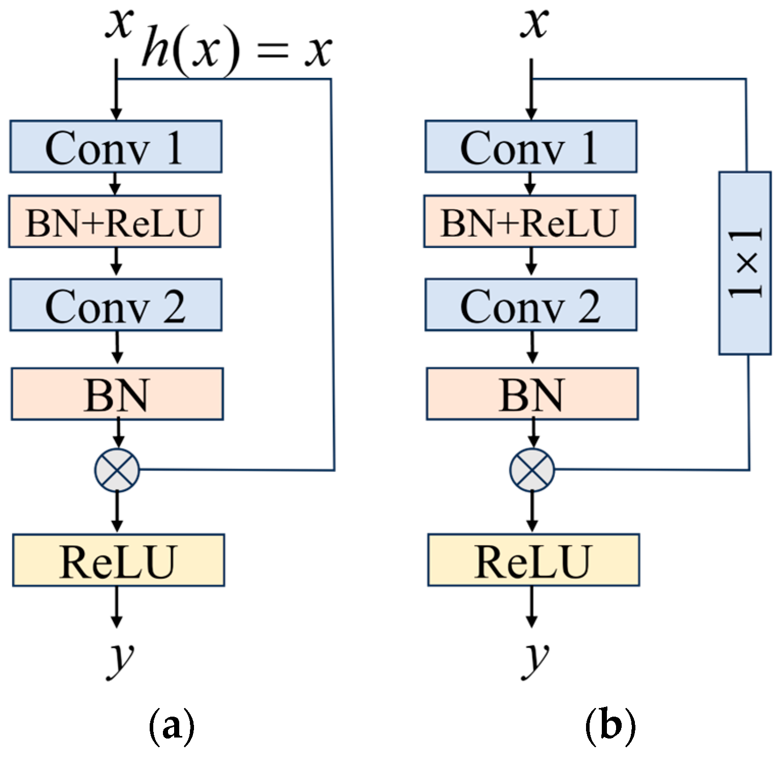
2.3.2. Residual Structure

In neural networks, the introduction of a residual structure through shortcut connections that skip one or more layers allows the input to be directly added to the network’s output. This design enables the network to focus on refining the input rather than learning an entirely new mapping technique, significantly diminishing training challenges, and mitigates issues such as gradient vanishing and explosion, which are common in networks with numerous convolutional and activation layers. Consequently, this approach enhances training convergence and simplifies the training process of deep networks. The typical configuration of a residual structure is depicted in Figure 2.

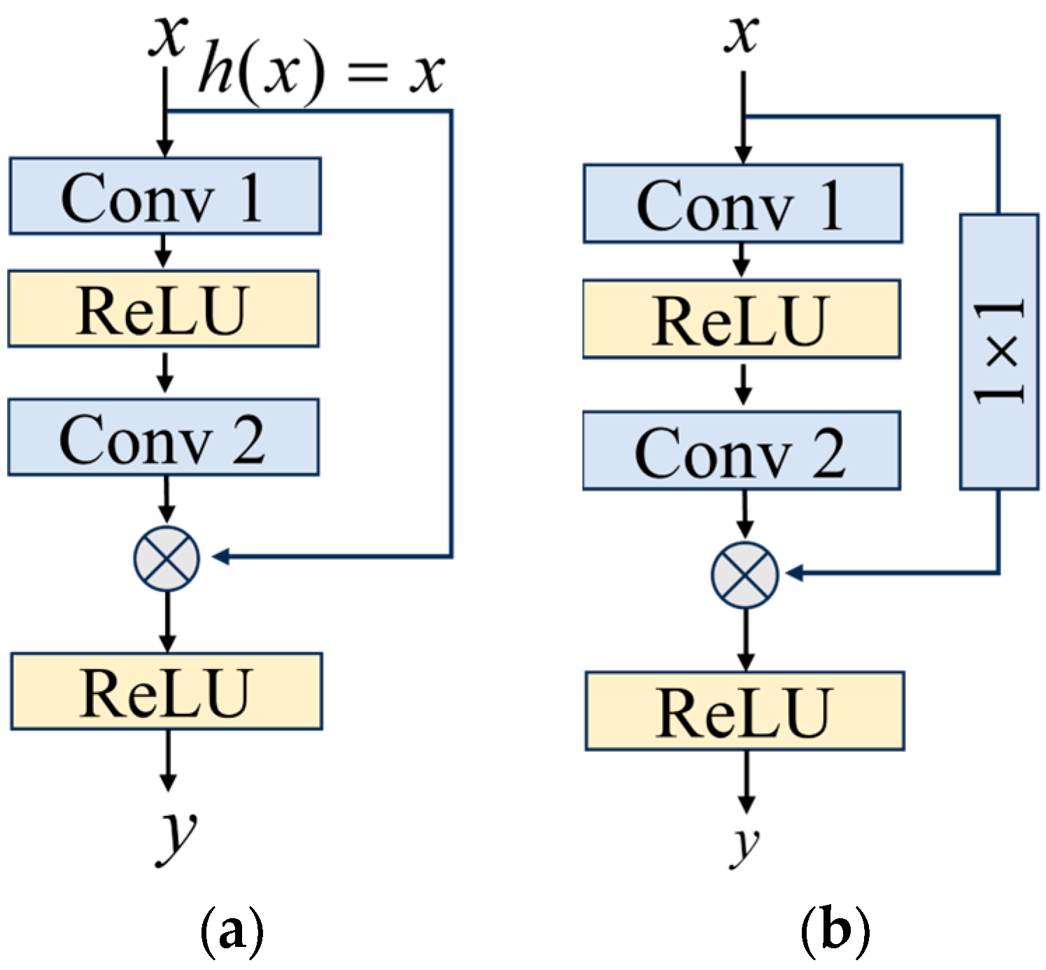
Mapping techniques can be categorized into the following two distinct methods based on the consistency of the input and output dimensions: identity mapping and projection mapping. Identity mapping is employed when the dimensions align, while projection mapping is utilized to reconcile dimensional discrepancies. Simplifying shallow networks by eliminating BN layers reduces the parameter count, accelerating training without increasing computational complexity. This adjustment makes the model more adaptable to small-scale datasets. Figure 3 illustrates the residual structure implemented in further experiments.

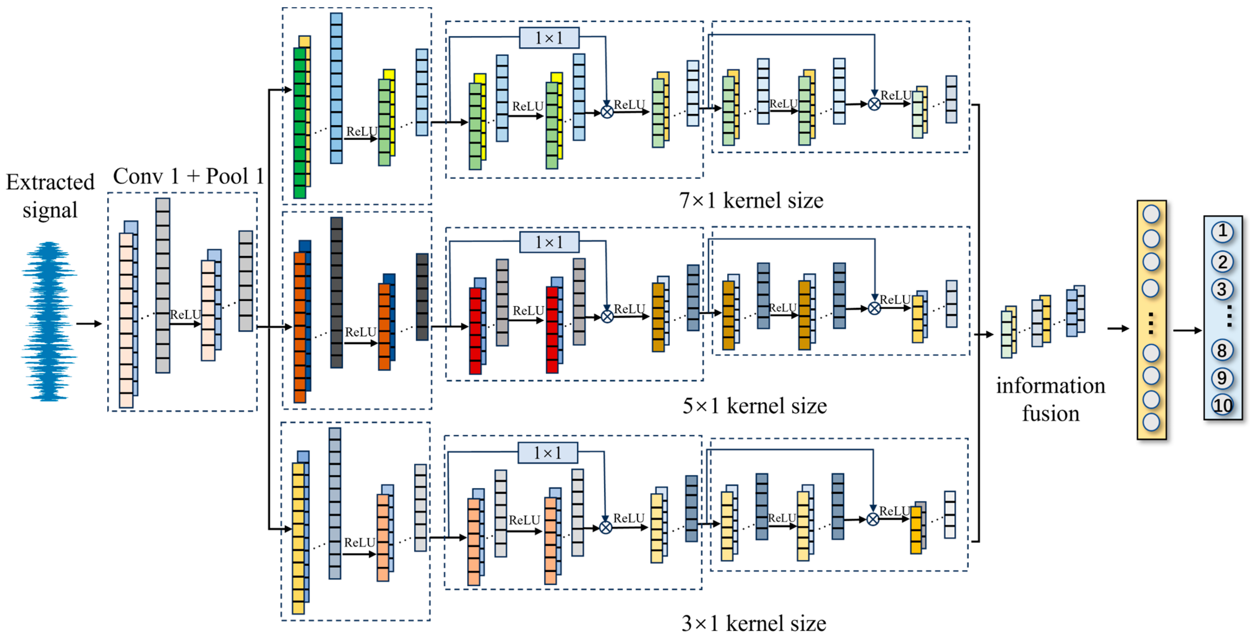
2.3.3. One-Dimensional Multi-Scale Residual Convolutional Neural Network

Utilizing convolution kernels of varying sizes to construct a multi-scale fusion CNN enables the integration of information across different scales. Initially, the network employs a large convolution kernel in its first layer to extract basic features from the vibration signal. Subsequently, convolution kernels of sizes 7 × 1, 5 × 1, and 3 × 1 are deployed in parallel to obtain more in-depth knowledge on the signal’s features. This approach not only facilitates the fusion of information, but also incorporates modified residual blocks to expedite convergence. Following this, the GAP layer processes the extracted features, leading to the final classification stage performed by the Softmax layer. The structure of the one-dimensional multi-scale residual convolutional neural network is shown in Figure 4. The parameters of the 1D-MRCNN are shown in

Table 1. The parameters of the 1D-MRCNN.

Layers	Kernel Width	Steps	Convolution Kernels	Features of the Output
Input	2048 × 1	-	-	-
Conv1	32 × 1	16 × 1	16	128 × 16
Pool1	2 × 1	2 × 1	16	64 × 16
Conv7(5,3)_1	7 × 1 (5 × 1, 3 × 1)	1 × 1	16	64 × 16
Pool7(5,3)_1	2 × 1	2 × 1	16	32 × 16
Conv7(5,3)_2	7 × 1 (5 × 1, 3 × 1)	1 × 1	32	32 × 32
Pool7(5,3)_2	2 × 1	2 × 1	32	16 × 32
Conv7(5,3)_3	7 × 1 (5 × 1, 3 × 1)	1 × 1	64	16 × 64
Pool7(5,3)_3	2 × 1	2 × 1	64	8 × 64
GAP	-	-	-	192
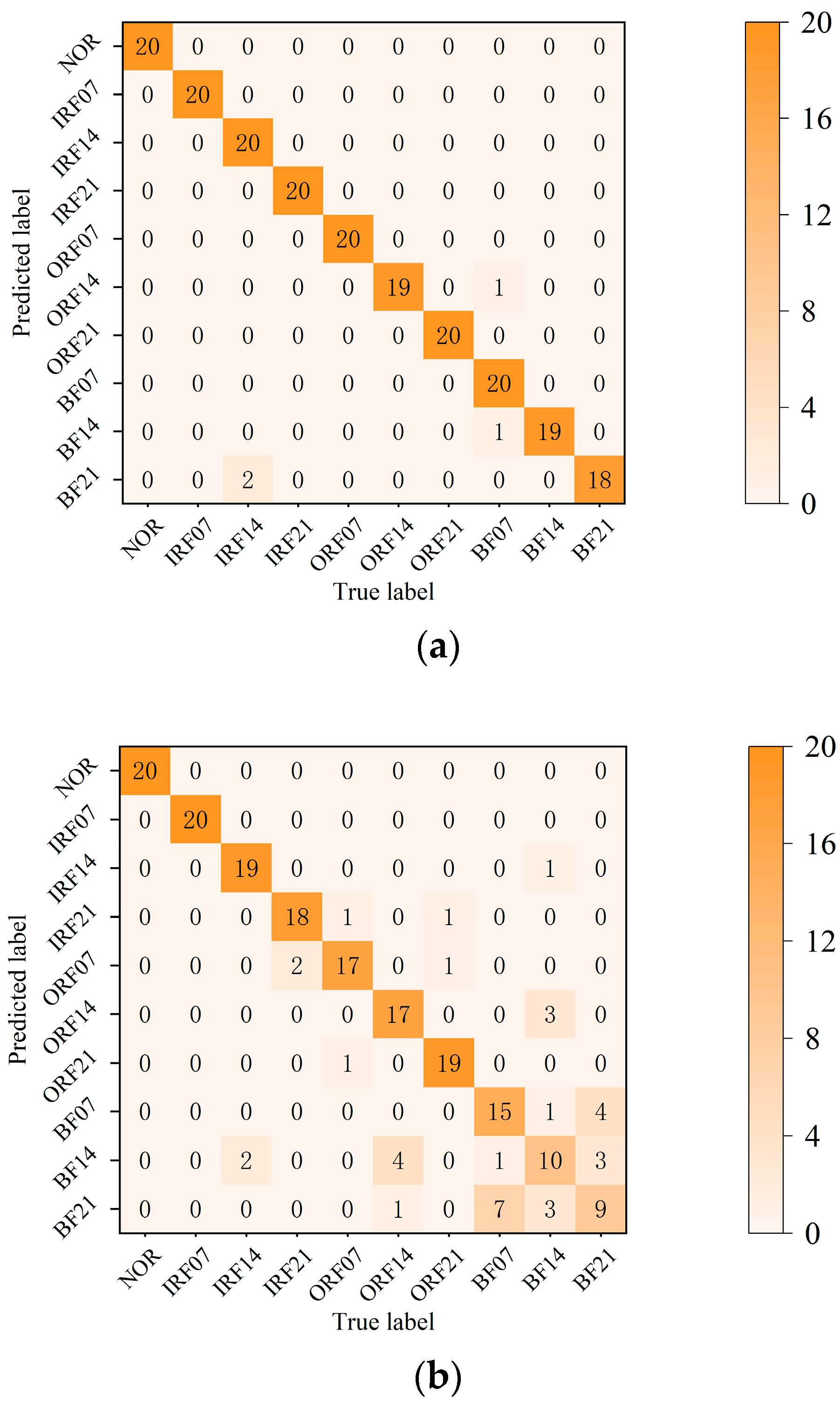
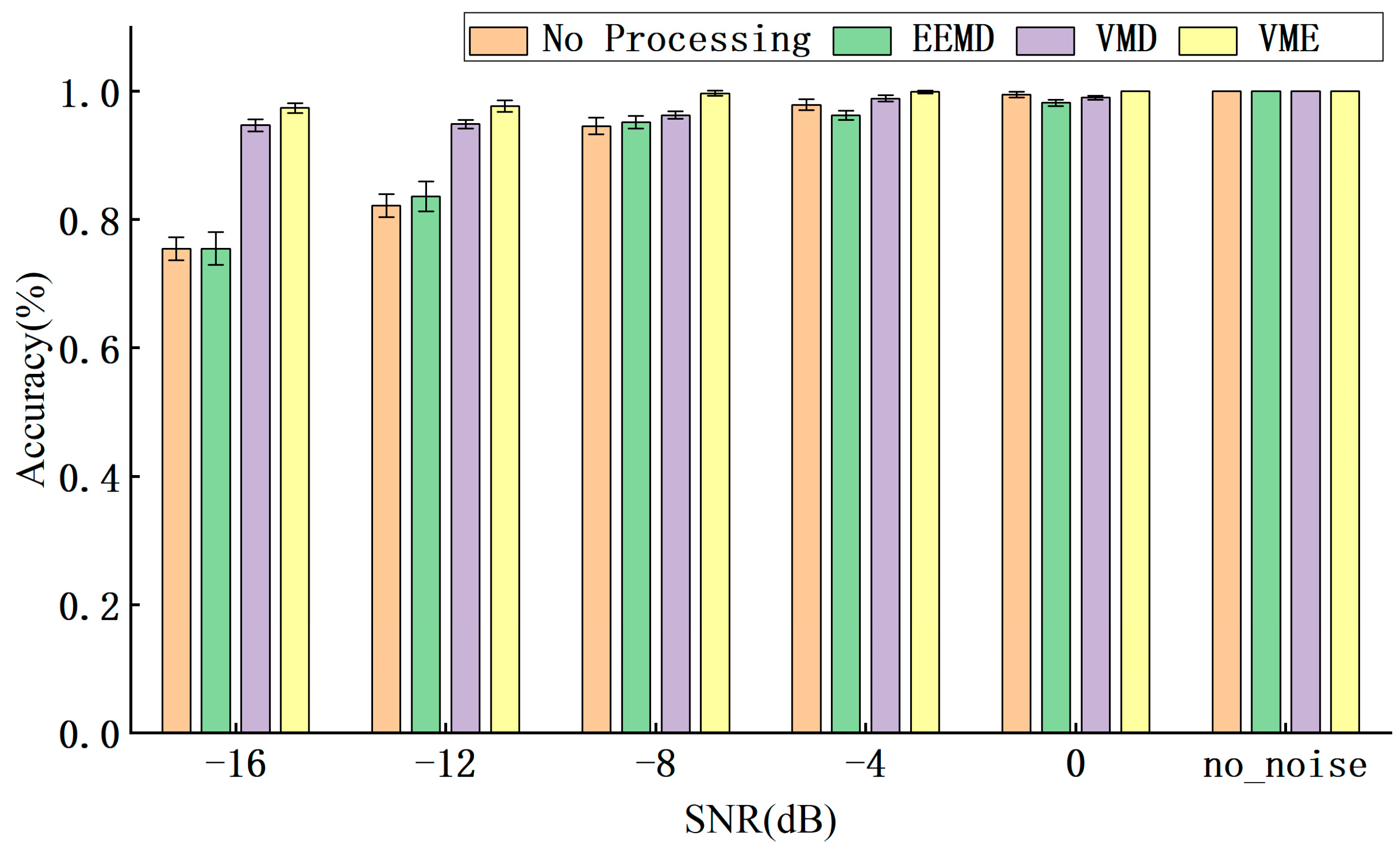
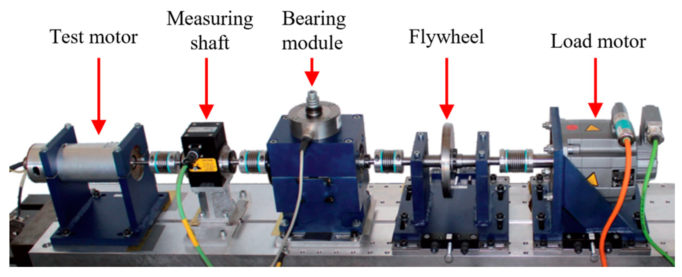
Softmax	-	-	-	10

. The vibration signal extracted using parameter-optimized VME will be converted into a dataset for input into the 1D-MRCNN.

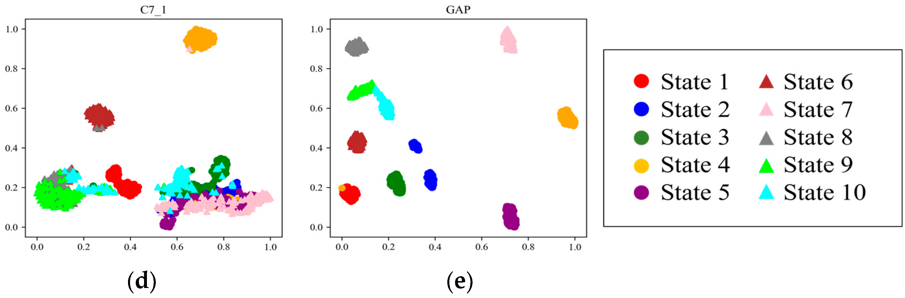
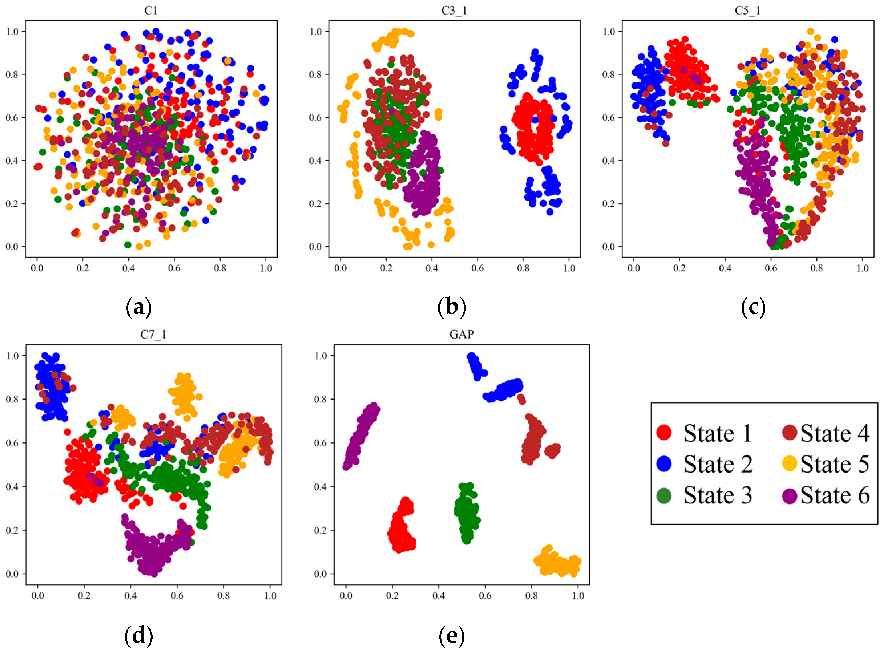
3. Fault Simulation Signal Analysis

In order to illustrate the effectiveness of the algorithm in this paper, a rolling bearing fault model is constructed to simulate the inner fault, and random shocks, periodic harmonics and Gaussian white noise are added, and the simulated signals are constructed as follows:

$$\left\{\begin{array}{l}\mathrm{x}(\mathrm{t})={\mathrm{x}}_1(\mathrm{t})+{\mathrm{x}}_2(\mathrm{t})+{\mathrm{x}}_3(\mathrm{t})+\mathrm{n}(\mathrm{t})\hfill \\ {\mathrm{x}}_1(\mathrm{t})={\displaystyle \sum _{\mathrm{i}}{\mathrm{A}}_{\mathrm{i}}}{\mathrm{s}}_{\mathrm{i}}\left(\mathrm{t}-\mathrm{i}{\mathrm{T}}_{\mathrm{a}}-{\mathsf{\tau }}_{\mathrm{i}}\right)\hfill \\ {\mathrm{x}}_2(\mathrm{t})={\displaystyle \sum _{\mathrm{j}}{\mathrm{B}}_{\mathrm{j}}}{\mathrm{s}}_{\mathrm{j}}\left(\mathrm{t}-\mathrm{j}{\mathrm{T}}_{\mathrm{b}}\right)\hfill \\ {\mathrm{x}}_3(\mathrm{t})={\displaystyle \sum _{\dot{\mathrm{k}}}{\mathrm{P}}_{\mathrm{k}}}\sin \left(2\mathsf{\pi }{\mathrm{f}}_{\mathrm{k}}\mathrm{t}+{\mathsf{\phi }}_{\mathrm{k}}\right)\hfill \end{array}\right.$$

(27)

In Equation (27), $\mathrm{x}(\mathrm{t})$ represents the mixed signal; ${\mathrm{x}}_1(\mathrm{t})$ represents the bearing inner fault; ${\mathrm{x}}_2(\mathrm{t})$ represents the random shocks caused by electromagnetic interference or the external environment; ${\mathrm{x}}_3(\mathrm{t})$ represents periodic harmonics; $\mathrm{n}(\mathrm{t})$ represents Gaussian white noise; $\mathrm{A}$, $\mathrm{B}$, and $\mathrm{P}$ denote different amplitudes; $\mathrm{T}$ denotes the interval between two adjacent pulses; $\mathsf{\tau }$ represents the small fluctuations caused by random sliding of the rolling element, which accounts for 1% of $\mathrm{T}$; ${\mathrm{f}}_{\mathrm{k}}$ denotes the frequency of the periodic harmonics; ${\mathsf{\phi }}_{\mathrm{k}}$ denotes the phase of the periodic harmonics; and $\mathrm{s}(\mathrm{t})$ denotes the impulse response function. The expression of $\mathrm{A}$ is as follows:

$$\mathrm{A}=1+{\mathrm{A}}_0\cos (2\mathsf{\pi }{\mathrm{f}}_{\mathrm{r}}\mathrm{t})$$

(28)

In Equation (28), ${\mathrm{f}}_{\mathrm{r}}$ denotes the frequency conversion.

The expression of $\mathrm{s}(\mathrm{t})$ is as follows:

$$\mathrm{s}(\mathrm{t})={\mathrm{e}}^{-{\mathrm{C}}_{\mathrm{n}}\mathrm{t}}\cos (2\mathsf{\pi }{\mathrm{f}}_{\mathrm{n}}\mathrm{t}+\mathsf{\phi })$$

(29)

In Equation (29), ${\mathrm{f}}_{\mathrm{n}}$ denotes the resonant frequency, $\mathsf{\phi }$ denotes the phase position, and ${\mathrm{C}}_{\mathrm{n}}$ denotes the attenuation coefficient.

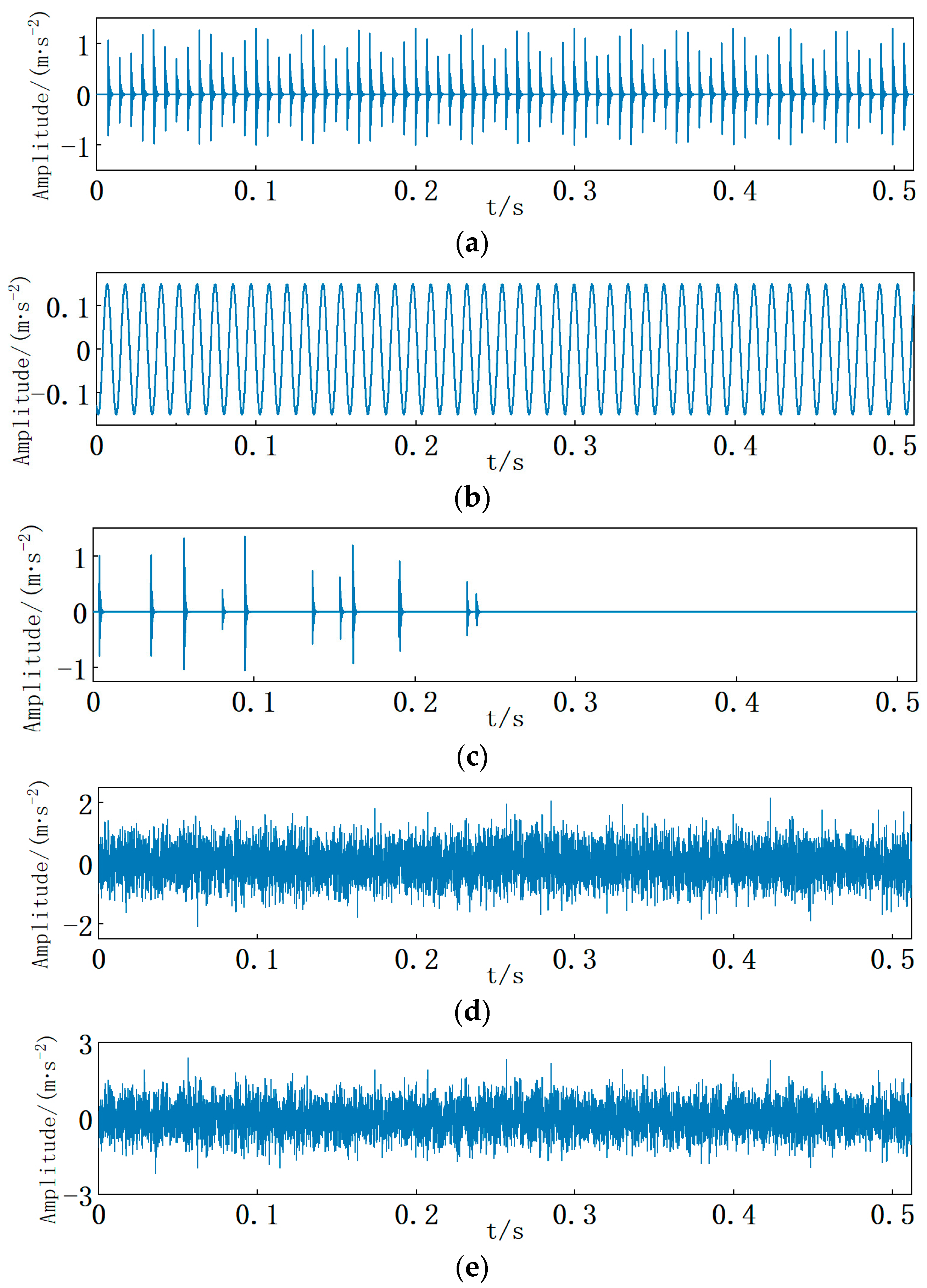
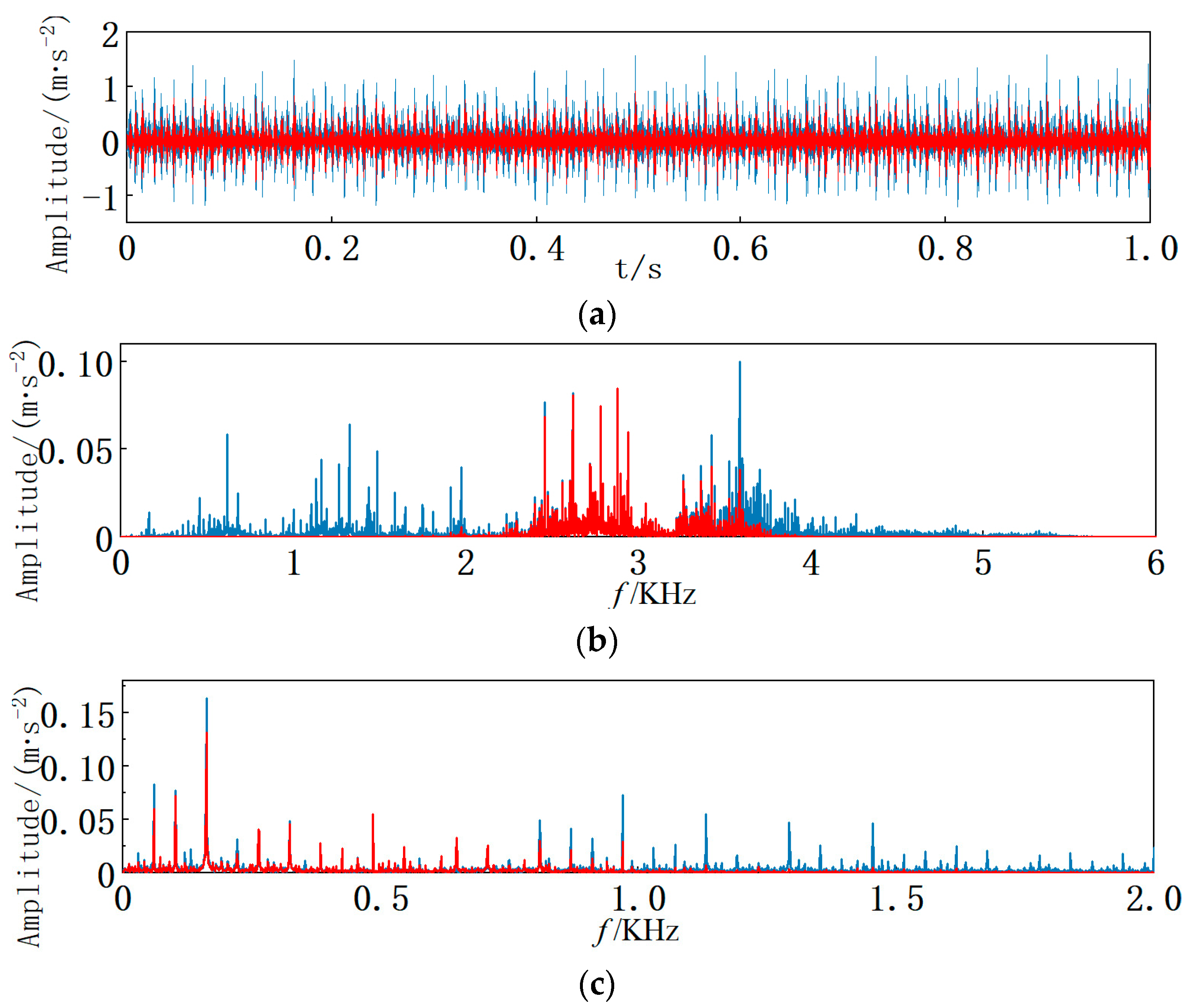
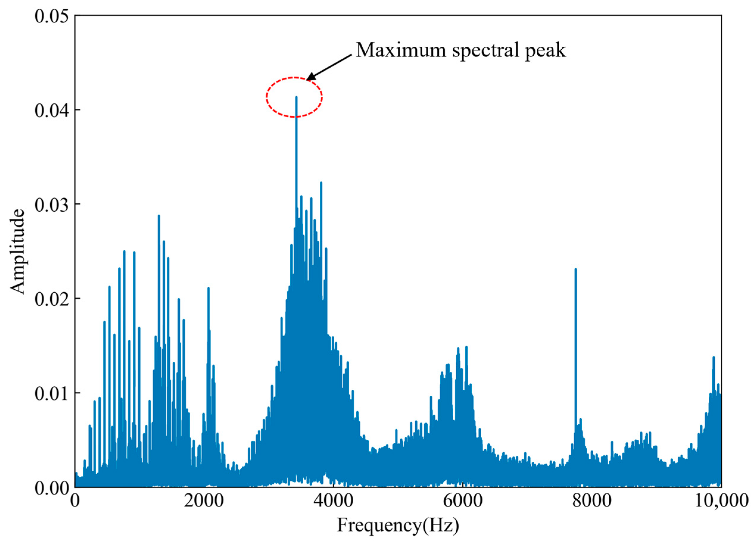
The inner fault simulation signal constructed in this paper is shown in Figure 5. The key parameters are as follows: the sampling frequency ${\mathrm{f}}_{\mathrm{s}}$ is set to 16 kHz, the sampling number to 8192, and the frequency conversion ${\mathrm{f}}_{\mathrm{r}}$ to 30 Hz, and the inner fault characteristic frequency is ${\mathrm{f}}_{\mathrm{i}}=1/{\mathrm{T}}_{\mathrm{a}}=140\mathrm{Hz}$. The resonance frequencies of the inner fault and random shocks are 3500 Hz and 4000 Hz, respectively. The attenuation coefficients are 800 and 2000, respectively. ${\mathrm{A}}_{\mathrm{o}}$ is set to 0.3, $\mathrm{B}$ is a random number in the range [0.25,1.25], $\mathrm{P}$ is set to 0.15, ${\mathrm{T}}_{\mathrm{b}}$ is a random number in the range [100,200], and $\mathrm{n}(\mathrm{t})$ is set to −10 dB of Gaussian white noise.

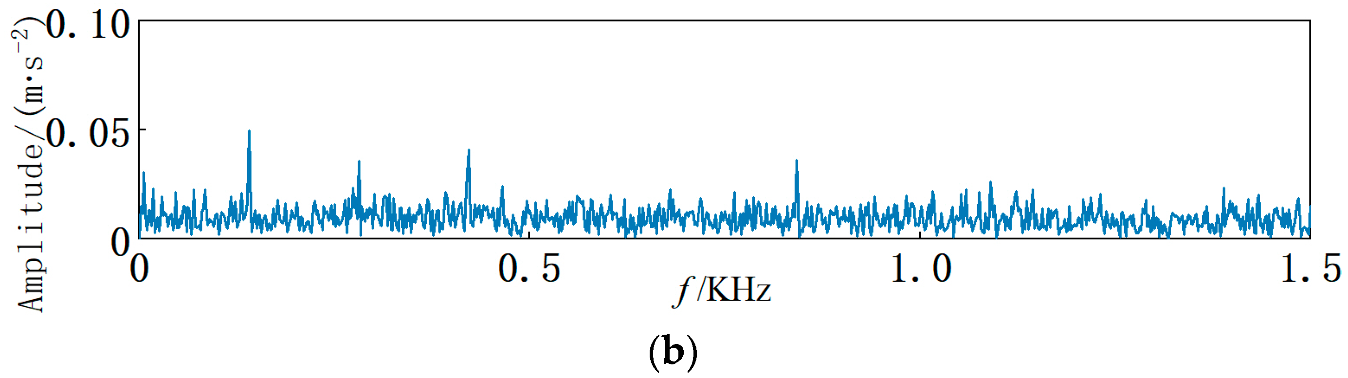
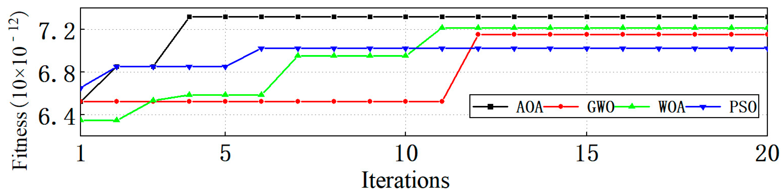
Signal and envelope spectrum diagrams of the inner fault are represented in Figure 6. To accurately identify the type of rolling bearing fault, the parameter-optimized VME method was employed for signal analysis. Firstly, the parameter $[\mathsf{\alpha },\mathsf{\omega }]$ in the VME algorithm was optimized, and the variation curve of WCK with respect to the number of iterations is shown in Figure 7.

After applying the AOA, the best parameter combination is determined to be [265,4271]. Further validation of the AOA’s efficiency for parameter optimization was conducted through comparative iterative optimization with the grey wolf algorithm (GWO), the whale optimization algorithm (WOA), and particle swarm optimization (PSO). The comparison reveals that the fitness values of the AOA, GWO, WOA, and PSO after the 4th, 12th, 11th, and 6th generations are 7.31, 7.15, 7.21, and 7.02, respectively (unit: 10 × 10⁻¹²).

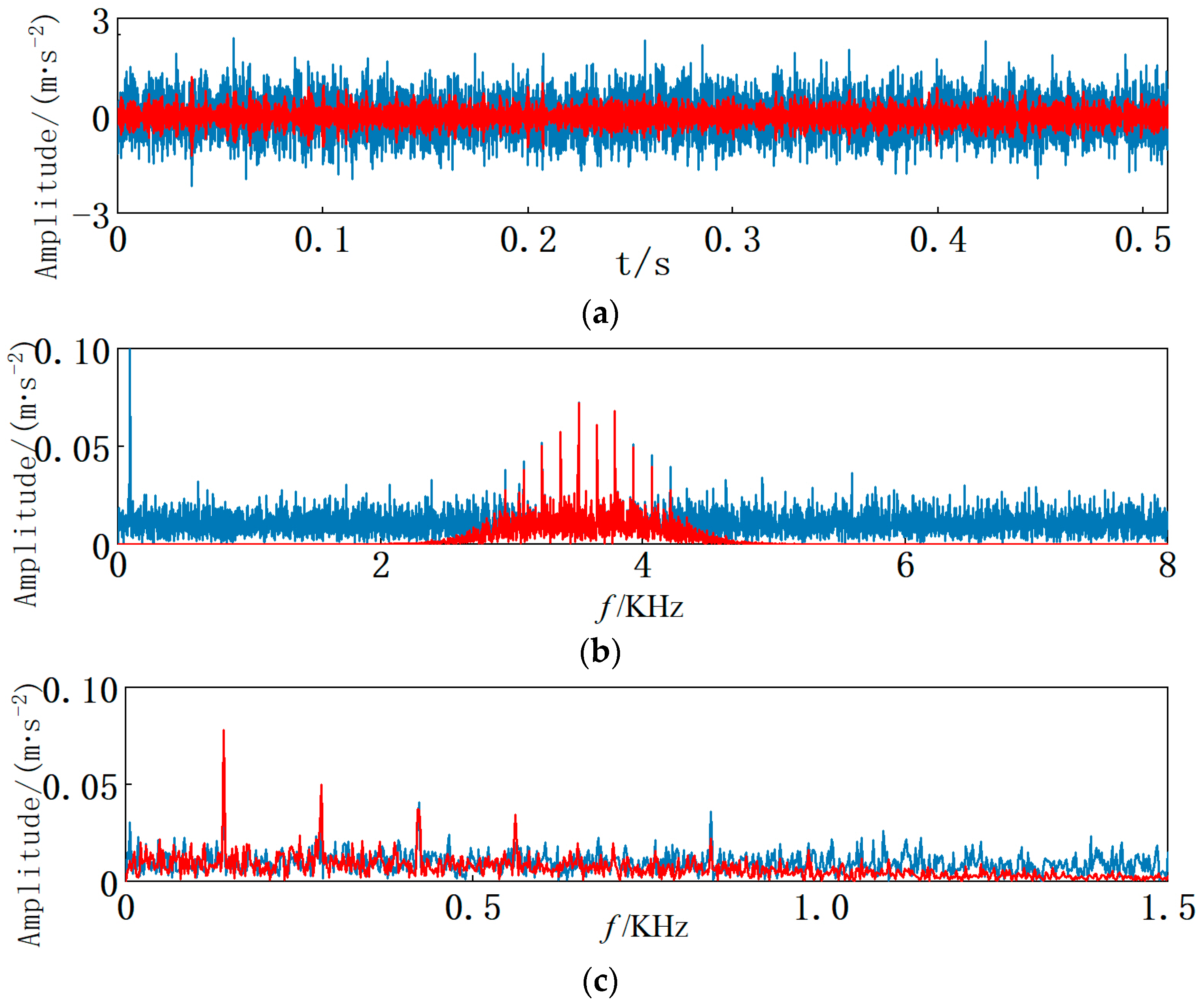
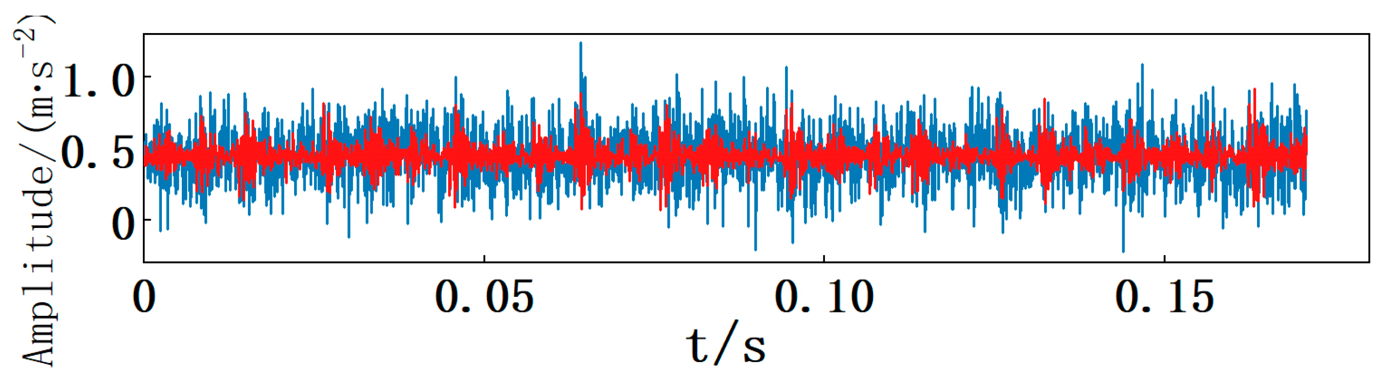
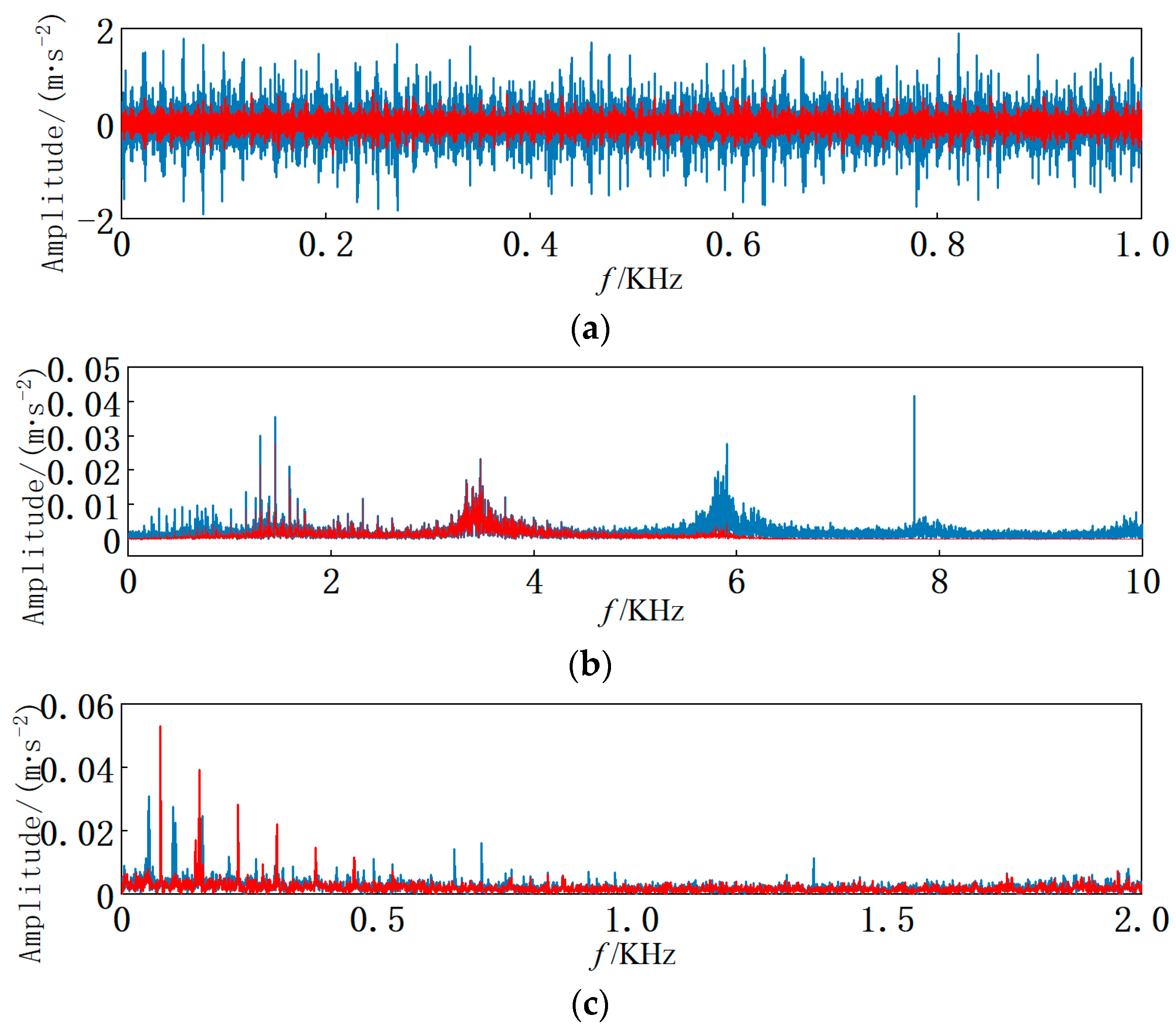
This analysis demonstrates that the AOA converges more rapidly and is less prone to becoming trapped in the local optimal solution. The results of the parameter-optimized VME are shown in Figure 8. Where the blue portion indicates the original signal, while the red portion indicates the extracted signal. The envelope spectrum reveals the inner fault frequency, accompanied by significant frequency doubling. The use of WCK as the objective function to optimize the VME parameters is demonstrated to be rational.

4. Fault Experiment Signal Analysis

A flow chart of the IVME-MRCNN is shown in Figure 9.

The steps are as follows:

• The vibration signal is acquired from the rolling bearing.
• The vibration signal is preprocessed by the parameter-optimized VME. The AOA is used to extract the signal from the optimal parameter [α, ω], where $\mathsf{\alpha }\in [0,10000]$ and $\mathsf{\omega }\in [0,\mathrm{f}\mathrm{s}/2]$, and the objective function is WCK.
• Dataset expansion is achieved through overlapping the sampling of the extracted signals with a 512-length sliding window. For each fault type, 200 samples are generated and randomly segmented into training, validation, and test sets, in specific ratios, with appropriate labels assigned to each data type.
• The training and validation sets are input into the 1D-MRCNN model for training. To ensure experimental fairness, the experiment is repeated five times using the average outcome as the final result.
• The test set is input into the trained 1D-MRCNN model to perform fault diagnosis classification.

4.1. Case Western Reserve University (CWRU) Dataset

4.1.1. Description of Experimental Equipment and Bearing Data

Data from the Electrical Engineering Laboratory at Case Western Reserve University were utilized to further demonstrate the effectiveness of the proposed method on actual rolling bearing fault signals [46]. The experimental setup, illustrated in Figure 10, included an electric motor, a torque transducer, and a dynamometer, etc.

Table 2. Rolling bearing parameters.

Bearing Type	Bearing Diameter/mm	Inner Diameter/mm	Outer Diameter/mm	Roller Diameter/mm	Number of Rollers	Contact Angle/(°)
SKF6205-2RS	39.04	25	52	7.94	9	0

displays the dimensional parameters of the test bearing. An accelerometer, with a sampling frequency of 12 kHz, was installed on the electric motor. In the experiment, an EDM at 1797 r/min was used to induce three single-point faults on the bearing: an inner fault, an outer fault, and a ball fault. Each fault type was characterized by three diameters, namely the early (0.1778 mm), middle (0.3556 mm), and late (0.5334 mm) stages, resulting in nine different states and one healthy state (see

Table 3. Details of CWRU dataset.

Fault Type	Fault Diameter (mm)	Number of Samples	Label
Normal (N)	0	200	0
Inner Fault 1 (IRF1)	0.1778	200	1
Inner Fault 2 (IRF2)	0.3556	200	2
Inner Fault 3 (IRF3)	0.5334	200	3
Outer Fault 1 (ORF1)	0.1778	200	4
Outer Fault 2 (ORF2)	0.3556	200	5
Outer Fault 3 (ORF3)	0.5334	200	6
Ball Fault 1 (BF1)	0.1778	200	7
Ball Fault 2 (BF2)	0.3556	200	8
Ball Fault 3 (BF3)	0.5334	200	9

). The acquired samples were allocated into training, validation, and test sets, with ratios of 70%, 20%, and 10%, respectively.

4.1.2. Experimental Validation

Firstly, the AOA optimizes the VME parameters $[\mathsf{\alpha },\mathsf{\omega }]$ to extract the desired mode components from the original vibration signals. For example, considering inner fault 1, the optimal parameter combination is [203, 2524]. The results of the parameter-optimized VME are shown in Figure 11. The signal undergoes decomposition during VME by optimizing the parameters $[\mathsf{\alpha },\mathsf{\omega }]$, based on the optimal combination identified in

Table 4. Optimal parameter combination for VME.

Fault Type	$[\mathbf{\alpha },\mathbf{\omega }]$	Fault Type	$[\mathbf{\alpha },\mathbf{\omega }]$
Normal	[726, 1497]	ORF2	[877, 4296]
IRF1	[203, 2524]	ORF3	[201, 2370]
IRF2	[378, 1892]	BF1	[2271, 3459]
IRF3	[200, 4865]	BF2	[2778, 3088]
ORF1	[2847, 765]	BF3	[386, 2333]

.

The neural network parameters were set as follows: the number of Softmax classification layers corresponded to the total number of fault types, which was 10. For the training set, the parameters were configured with an Adam optimizer learning rate of 0.002, a batch size of 32, and a maximum of 100 training iterations, and the chosen loss function was categorical cross-entropy. To demonstrate the need to remove the residual structure of the BN layer, we compared a model with the BN layer removed, a model retaining the BN layer, and an MSCNN without the residual structure; the results are displayed in Figure 12. The training and validation sets achieve a steady state after four iterations in the model without the BN layer’s residual structure. While all three models achieve 100% accuracy, the model lacking the BN layer’s residual structure exhibits the best convergence. The confusion matrix is shown in Figure 13.

4.1.3. Experiment Validation in Noisy Environments

To further validate the effectiveness of the method in noisy environments, Gaussian white noise was introduced into the bearing vibration signals. Noisy datasets with signal-to-noise ratios of −16 dB, −12 dB, −8 dB, −4 dB, and 0 dB were generated. Figure 14 illustrates the mixed signal resulting from the addition of noise.

In order to demonstrate the effectiveness and superiority of the IVME-MRCNN method, we processed the same experimental data with the MRCNN, akin to a traditional CNN and MSCNN, and compared it with the non-parameter-optimized VME method. The outcomes are displayed Figure 15. Parameter-optimized VME significantly enhances the overall accuracy when analyzing noisy bearing signal data, particularly at noise levels of −16 dB and −12 dB. As the SNR decreases, all six methods experience a drop in accuracy. However, the IVME-MRCNN demonstrates superior robustness, maintaining an accuracy of 97.7 ± 0.93 (%), even in the −16 dB environment.

To enhance the intuitiveness of the feature learning process in the proposed method, t-distributed Stochastic Neighbor Embedding (t-SNE) was employed to transform high-dimensional features into two-dimensional ones, facilitating the visualization of different network layers. The results are shown in Figure 16. Figure 16a provides a visualization of the original data. The points, representing various bearing faults and differentiated by color, are scattered and challenging to distinguish. Figure 16b–d provides a visualization of the results for the three distinct branches, where points within the same category appear more clustered. Figure 16e presents the results after global average pooling, where points in the same category are clustered, with only a few outliers, demonstrating the MRCNN’s feature extraction capability.

To demonstrate the benefits of parameter-optimized VME, we compared it to the approach by Ye et al. [26], who employed a fixed α value of 1000. The selection was based on the frequency value corresponding to the highest spectral peak in the bearing vibration signal. The selected values are shown in

Table 5. The center frequency of the bearing vibration signal for different fault types.

Fault Type	$\mathbf{\omega }$/Hz	Fault Type	$\mathbf{\omega }$/Hz
Nor	1000	ORF14	3400
IRF07	3500	ORF21	3400
IRF14	3500	BF07	3400
IRF21	2800	BF14	3400
ORF07	2800	BF21	3400

.

Table 6. Accuracy of parameter-optimized VME and empirical VME within the MRCNN model.

Parameter Optimized	No Noise	0 dB	−4 dB	−8 dB	−12 dB	−16 dB
Yes	100 ± 0	100 ± 0	99.9 ± 0.1	99.7 ± 0.4	97.7 ± 0.93	97.4 ± 0.74
No	99.9 ± 0.2	99.1 ± 0.2	98.0 ± 0.5	95.9 ± 1.0	84.8 ± 1.3	82.8 ± 2.5

presents the results of the comparison between the parameter-optimized VME and empirical VME, within the MRCNN model. The signal features extracted using parameter-optimized VME are more obvious than those extracted using empirical VME. In the case of no noise, 0 dB and −4 dB, the accuracy of VME using the empirical method is also close to 100%. As the SNR decreases further, the advantages of signal extraction using parameter-optimized VME become more evident. Figure 17 displays confusion matrixes for both methods at −16 dB. The diagnostic accuracy, as shown in the confusion matrixes, is significantly enhanced with parameter-optimized VME.

The impact of the signal preprocessing method (VMD, EEMD) on the results were analyzed. VMD employs WCK as the objective function for signal decomposition, selecting the IMF’s mode component with the maximum WCK value as the optimal component. In EEMD decomposition, the noise amplitude ratio is set to $\mathsf{\epsilon }=0.2$ relative to the signal amplitude’s standard deviation, with N = 100 trials conducted, and mode component 1 is selected as the principal component. Hence, the results indicate that preprocessing the noisy original vibration signal with parameter-optimized VME can enhance accuracy and save time.

Table 7. The average time of each decomposition using different signal preprocessing methods.

Methods	VME	VMD	EEMD
Time(s)	0.02	4.32	4.98

presents the average decomposition time for each signal preprocessing method. Figure 18 illustrates the results from employing different signal preprocessing methods within the MRCNN. With parameter-optimized VME, the MRCNN demonstrates robustness as the SNR decreases. While parameter-optimized VMD is less robust compared to VME, and EEMD shows minimal improvement in terms of accuracy, both methods have longer running times than VME. These results indicate that preprocessing the noisy original vibration signal with parameter-optimized VME can enhance accuracy and save time.

4.2. Paderborn University (PU) Dataset

4.2.1. Description of Experimental Equipment and Bearing Data

The experimental data were provided by the Design and Drive Technology Center at Paderborn University. The test rig comprised basic components, such as a test motor, measuring shaft, bearing module, flywheel, and load motor, as illustrated in Figure 19. The failures included both human damage and accelerated experimental damage. Artificial damage was inflicted using traditional processing techniques such as drilling, EDM, and an electric engraver. The experiment included healthy conditions, as well as inner, outer, and compound faults. The stator current and vibration signals were collected using a current sensor and a piezoelectric accelerometer, respectively, with a 64 K sampling frequency and 4 s per sample, and the experiment included a total of 2560 samples. The test conditions included varying speeds of 900 r/min and 1500 r/min, loads of 0.1 Nm and 0.7 Nm, and radial forces of 1000 N and 400 N, and vibration signals recorded at radial forces of 1500 r/min, 0.7 Nm load, and 1000 N were utilized as the experimental dataset. Six distinct fault types were analyzed: healthy, IR1 (inner ring damage degree 1), IR2 (inner ring damage degree 2), OR1 (outer ring damage degree 1), OR2 (outer ring damage degree 2), and compound faults involving both the inner and outer rings.

For each fault type, 200 samples were allocated to training, validation, and test sets in 60%, 20%, and 20% ratios, respectively.

Table 8. Details of PU dataset.

Fault Type	Fault Level	Number of Samples	Level
Normal (N)	/	200	0
Inner Fault 1	1	200	1
Inner Fault 2	2	200	2
Outer Fault 1	1	200	3
Outer Fault 2	2	200	4
Compound	/	200	5

displays the bearing dataset details. Firstly, the AOA optimized the VME parameters $[\mathsf{\alpha },\mathsf{\omega }]$ to extract the desired mode components from the original vibration signals. Take outer fault 2 as an example; the best parameter combination identified is [2616, 4084]. Figure 20 illustrates the results of the parameter-optimized VME. In regard to the time-domain signal processed by the optimally parameterized VME, more impact components are observable. The interference spectrum lines around the fault characteristic frequency are significantly reduced in regard to the envelope spectrum. The signal is decomposed by optimizing $[\mathsf{\alpha },\mathsf{\omega }]$ in VME, according to the optimal parameter combination listed in

Table 9. Optimal parameter combination for VME.

Fault Type	$[\mathbf{\alpha },\mathbf{\omega }]$	Fault Type	$[\mathbf{\alpha },\mathbf{\omega }]$
Normal	[863, 1363]	ORF1	[1201, 2752]
IRF1	[1827, 2059]	ORF2	[2616, 4084]
IRF2	[807, 3917]	COM	[1186, 4051]

.

The divided training set and validation set are fed into the MRCNN for training. Figure 21 displays the training results, showing that the accuracy and loss curves stabilize after 15 iterations. The loss value approaches 0, while the accuracy approaches 100%. The test samples are input into the trained MRCNN for testing, with the outcomes depicted in the confusion matrix shown in Figure 22. Apart from one compound fault sample misclassified as inner fault 2, all other test samples are correctly identified, demonstrating the proposed method’s accuracy.

4.2.2. Experimental Validation in Noisy Environments

To validate the proposed method’s efficacy against noise, Gaussian white noise was introduced into the bearing vibration signal, creating noisy datasets at −16 dB, −12 dB, −8 dB, −4 dB, and 0 dB. The performance of the traditional CNN and MSCNN and the proposed MRCNN were compared, both with and without optimized VME parameters. The results are shown in Figure 23. At an SNR of 0 dB, the accuracy levels of the six methods are comparable, each surpassing 95% accuracy. However, with a further reduction in the SNR, the benefits of parameter-optimized VME preprocessing become increasingly evident. Additionally, the proposed MRCNN demonstrates higher recognition accuracy and greater robustness compared to the traditional CNN and MSCNN.

The impacts of parameter-optimized VME and empirical signal preprocessing on MRCNN training were compared using a fixed value of 1000 and a frequency corresponding to the highest spectral peak. ORF2 is used as an example, as shown in Figure 24. Figure 24a offers a graphical representation of the initial data. These points, indicative of different bearing faults and distinguished by color, are dispersed and difficult to identify. In Figure 24b–d, the outcomes for the three separate branches are visually represented, showing a greater clustering of points within the same category. In Figure 24e, the outcomes post-global average pooling are displayed, highlighting the clustering of points within the same category with minimal outliers, showcasing the MRCNN’s proficiency in extracting features.

Table 10. Center frequencies for different fault types.

Fault Type	$\mathbf{\omega }$/Hz	Fault Type	$\mathbf{\omega }$/Hz
Normal	1302	ORF1	3427
IRF1	1258	ORF2	7747
IRF2	1303	COM	532

displays the center frequencies associated with each fault type.

Table 11. Accuracy of parameter-optimized VME and empirical VME within MRCNN model.

Parameter Optimized	No Noise	0 dB	−4 dB	−8 dB	−12 dB	−16 dB
Yes	99.4 ± 0.2	98.5 ± 0.4	96.0 ± 0.2	95.8 ± 0.6	94.8 ± 0.5	94.4 ± 0.4
No	100 ± 0	99.5 ± 0.2	96.5 ± 0.6	94.3 ± 0.6	87.3 ± 0.6	77.3 ± 0.9

presents the comparison results for parameter-optimized VME and empirical VME within the MRCNN model. The choice of α for Empirical VME is the same as by Ye et al. [26], which is 1000. The frequency value corresponding to the highest spectral peak takes ORF2 in Figure 25 as an example. Under noise-free conditions and at 0 dB and −4 dB SNR levels, the accuracy of empirical VME slightly surpasses that of parameter-optimized VME. However, at lower SNR levels, parameter-optimized VME demonstrates greater robustness than empirical VME, maintaining an accuracy of 94.4 ± 0.4 (%) at −16 dB. In contrast, the accuracy of empirical VME drops to 77.3 ± 0.9 (%) at the same SNR level. Figure 26 illustrates the confusion matrixes for both methods at −16 dB, and it is demonstrated that parameter-optimized VME is significantly more effective in high-noise environments.

To further assess the impact of various signal preprocessing methods on the outcomes, the approach depicted in Figure 17 was applied. The results are shown in Figure 27. At no noise, 0 dB, and −4 dB, parameter-optimized VMD shows higher accuracy than parameter-optimized VME; however, VME is less time consuming and better suited to preprocessing multiple signal samples. At −8 dB and below, VME outperforms the other algorithms in terms of accuracy. Thus, parameter-optimized VME emerges as a more advantageous method for signal preprocessing.

5. Conclusions

This paper introduces a new method for fault feature extraction in rolling bearings that involves optimizing the parameters of VME with an AOA, and proposes a 1D-MRCNN model with an improved residual structure for the automatic identification of fault types in rolling bearings. Initially, the AOA is employed to optimize the parameters [α, ω] of VME, reduce noise in the original vibration signals, and extract fault features. Subsequently, the extracted vibration signals are divided into datasets and input into the 1D-MRCNN for training. Finally, a test is conducted to validate the proposed method’s fault classification accuracy, leading to the following conclusions:

(1)

In the optimization of the VME parameters with the AOA, weighted correlated kurtosis (WCK) is employed as the objective function. Both simulated and experimental signals demonstrate that this objective function can effectively extract fault information, confirming that this method enhances the accuracy of fault feature extraction in noisy environments. Through comparative analysis with other optimization algorithms, it has been demonstrated that AOA exhibits superior capabilities when addressing complex problems prone to local optimal solutions. This lays a foundation for subsequent fault classification in rolling bearings.

(2)

A multi-scale residual convolutional neural network is proposed. Compared with the traditional CNN and MSCNN, it can be concluded that a multi-scale convolution kernel can more effectively achieve information complementarity at different scales, a gap layer can reduce the number of network parameters, and an improved residual structure can improve the training speed, and improve the accuracy of fault recognition.

(3)

Upon comparing parameter-optimized VME with empirical VME, parameter-optimized VMD, EEMD, and unprocessed vibration signals, it is revealed that parameter-optimized VME retains higher recognition accuracy than empirical VME, EEMD, and unprocessed vibration signals in noisy environments. Compared with parameter-optimized VMD, it offers a low computational cost and reduced processing time. This underlines its clear advantages over other algorithms.

(4)

The computational efficiency of the proposed method, although improved, still poses challenges when deployed in real-time monitoring systems, particularly in resource-constrained environments. Future work will aim to address these limitations by exploring more adaptive signal processing techniques and further refining the network architecture to enhance its applicability and efficiency in a broader range of operational contexts.

References

1. Jiao, J.; Zhao, M.; Lin, J.; Liang, K. Hierarchical discriminating sparse coding for weak fault feature extraction of rolling bearings. Reliab. Eng. Syst. Saf. 2019, 184, 41–54. [Google Scholar] [CrossRef]
2. Shi, H.; Hou, M.; Wu, Y.; Li, B. Incipient Fault Detection of Full Ceramic Ball Bearing Based on Modified Observer. Int. J. Control Autom. Syst. 2022, 20, 727–740. [Google Scholar] [CrossRef]
3. Gao, S.; Han, Q.; Zhang, X.; Pennacchi, P.; Chu, F. Ultra-high-speed hybrid ceramic triboelectric bearing with real-time dynamic instability monitoring. Nano Energy 2022, 103, 107759. [Google Scholar] [CrossRef]
4. Jin, Z.; He, D.; Wei, Z. Intelligent fault diagnosis of train axle box bearing based on parameter optimization VMD and improved DBN. Eng. Appl. Artif. Intell. 2022, 110, 104713. [Google Scholar] [CrossRef]
5. Moore, K.J.; Kurt, M.; Eriten, M.; McFarland, D.M.; Bergman, L.A.; Vakakis, A.F. Wavelet-bounded empirical mode decomposition for measured time series analysis. Mech. Syst. Signal Process. 2018, 99, 14–29. [Google Scholar] [CrossRef]
6. Gao, Y.; Villecco, F.; Li, M.; Song, W. Multi-Scale Permutation Entropy Based on Improved LMD and HMM for Rolling Bearing Diagnosis. Entropy 2017, 19, 176. [Google Scholar] [CrossRef]
7. Guo, W.; Tse, P.W. A novel signal compression method based on optimal ensemble empirical mode decomposition for bearing vibration signals. J. Sound Vib. 2013, 332, 423–441. [Google Scholar] [CrossRef]
8. Hu, C.; Xing, F.; Pan, S.; Yuan, R.; Lv, Y. Fault Diagnosis of Rolling Bearings Based on Variational Mode Decomposition and Genetic Algorithm-Optimized Wavelet Threshold Denoising. Machines 2022, 10, 649. [Google Scholar] [CrossRef]
9. Wang, L.; Liu, Z.; Miao, Q.; Zhang, X. Time–frequency analysis based on ensemble local mean decomposition and fast kurtogram for rotating machinery fault diagnosis. Mech. Syst. Signal Process. 2018, 103, 60–75. [Google Scholar] [CrossRef]
10. Dragomiretskiy, K.; Zosso, D. Variational Mode Decomposition. IEEE Trans. Signal Process. 2014, 62, 531–544. [Google Scholar] [CrossRef]
11. Jiang, X.; Wang, J.; Shen, C.; Shi, J.; Huang, W.; Zhu, Z.; Wang, Q. An adaptive and efficient variational mode decomposition and its application for bearing fault diagnosis. Struct. Health Monit. 2020, 20, 2708–2725. [Google Scholar] [CrossRef]
12. Wang, Y.; Markert, R.; Xiang, J.; Zheng, W. Research on variational mode decomposition and its application in detecting rub-impact fault of the rotor system. Mech. Syst. Signal Process. 2015, 60–61, 243–251. [Google Scholar] [CrossRef]
13. Li, K.; Su, L.; Wu, J.; Wang, H.; Chen, P. A Rolling Bearing Fault Diagnosis Method Based on Variational Mode Decomposition and an Improved Kernel Extreme Learning Machine. Appl. Sci. 2017, 7, 1004. [Google Scholar] [CrossRef]
14. Zhang, X.; Miao, Q.; Zhang, H.; Wang, L. A parameter-adaptive VMD method based on grasshopper optimization algorithm to analyze vibration signals from rotating machinery. Mech. Syst. Signal Process. 2018, 108, 58–72. [Google Scholar] [CrossRef]
15. Dibaj, A.; Hassannejad, R.; Ettefagh, M.M.; Ehghaghi, M.B. Incipient fault diagnosis of bearings based on parameter-optimized VMD and envelope spectrum weighted kurtosis index with a new sensitivity assessment threshold. ISA Trans. 2021, 114, 413–433. [Google Scholar] [CrossRef] [PubMed]
16. Wang, Q.; Yang, C.; Wan, H.; Deng, D.; Nandi, A.K. Bearing fault diagnosis based on optimized variational mode decomposition and 1D convolutional neural networks. Meas. Sci. Technol. 2021, 32, 104007. [Google Scholar] [CrossRef]
17. Wang, X.; Liu, X.; Wang, J.; Xiong, X.; Bi, S.; Deng, Z. Improved Variational Mode Decomposition and One-Dimensional CNN Network with Parametric Rectified Linear Unit (PReLU) Approach for Rolling Bearing Fault Diagnosis. Appl. Sci. 2022, 12, 9324. [Google Scholar] [CrossRef]
18. He, D.; Liu, C.; Jin, Z.; Ma, R.; Chen, Y.; Shan, S. Fault diagnosis of flywheel bearing based on parameter optimization variational mode decomposition energy entropy and deep learning. Energy 2022, 239, 122108. [Google Scholar] [CrossRef]
19. Gai, J.; Shen, J.; Hu, Y.; Wang, H. An integrated method based on hybrid grey wolf optimizer improved variational mode decomposition and deep neural network for fault diagnosis of rolling bearing. Measurement 2020, 162, 107901. [Google Scholar] [CrossRef]
20. Miao, Y.; Zhao, M.; Lin, J. Identification of mechanical compound-fault based on the improved parameter-adaptive variational mode decomposition. ISA Trans. 2019, 84, 82–95. [Google Scholar] [CrossRef]
21. Li, H.; Liu, T.; Wu, X.; Chen, Q. An optimized VMD method and its applications in bearing fault diagnosis. Measurement 2020, 166, 108185. [Google Scholar] [CrossRef]
22. Lyu, X.; Hu, Z.; Zhou, H.; Wang, Q. Application of improved MCKD method based on QGA in planetary gear compound fault diagnosis. Measurement 2019, 139, 236–248. [Google Scholar] [CrossRef]
23. McDonald, G.L.; Zhao, Q.; Zuo, M.J. Maximum correlated Kurtosis deconvolution and application on gear tooth chip fault detection. Mech. Syst. Signal Process. 2012, 33, 237–255. [Google Scholar] [CrossRef]
24. Yu, M.; Fang, M. Feature extraction of rolling bearing multiple faults based on correlation coefficient and Hjorth parameter. ISA Trans. 2022, 129 Pt B, 442–458. [Google Scholar] [CrossRef]
25. Nazari, M.; Sakhaei, S.M.; Nazari, M.; Sakhaei, S.M. Variational Mode Extraction: A New Efficient Method to Derive Respiratory Signals from ECG. IEEE J. Biomed. Health Inform. 2018, 22, 1059–1067. [Google Scholar] [CrossRef] [PubMed]
26. Ye, M.; Yan, X.; Chen, N.; Jia, M. Intelligent fault diagnosis of rolling bearing using variational mode extraction and improved one-dimensional convolutional neural network. Appl. Acoust. 2023, 202, 109143. [Google Scholar] [CrossRef]
27. Yan, X.; Xu, Y.; She, D.; Zhang, W. A Bearing Fault Diagnosis Method Based on PAVME and MEDE. Entropy 2021, 23, 1402. [Google Scholar] [CrossRef] [PubMed]
28. Liu, C.; Tan, J.; Huang, Z. Adaptive variational mode extraction method for bearing fault diagnosis based on window fusion. Measurement 2022, 202, 111856. [Google Scholar] [CrossRef]
29. Guo, X.; Chen, L.; Shen, C. Hierarchical adaptive deep convolution neural network and its application to bearing fault diagnosis. Measurement 2016, 93, 490–502. [Google Scholar] [CrossRef]
30. Saucedo-Dorantes, J.J.; Arellano-Espitia, F.; Delgado-Prieto, M.; Osornio-Rios, R.A. Diagnosis Methodology Based on Deep Feature Learning for Fault Identification in Metallic, Hybrid and Ceramic Bearings. Sensors 2021, 21, 5832. [Google Scholar] [CrossRef]
31. Wen, L.; Li, X.; Gao, L.; Zhang, Y. A New Convolutional Neural Network-Based Data-Driven Fault Diagnosis Method. IEEE Trans. Ind. Electron. 2018, 65, 5990–5998. [Google Scholar] [CrossRef]
32. Zhao, M.; Zhong, S.; Fu, X.; Tang, B.; Pecht, M. Deep Residual Shrinkage Networks for Fault Diagnosis. IEEE Trans. Ind. Inform. 2020, 16, 4681–4690. [Google Scholar] [CrossRef]
33. Chen, C.-C.; Liu, Z.; Yang, G.; Wu, C.-C.; Ye, Q. An Improved Fault Diagnosis Using 1D-Convolutional Neural Network Model. Electronics 2020, 10, 59. [Google Scholar] [CrossRef]
34. Lyu, P.; Zhang, K.; Yu, W.; Wang, B.; Liu, C. A novel RSG-based intelligent bearing fault diagnosis method for motors in high-noise industrial environment. Adv. Eng. Inform. 2022, 52, 101564. [Google Scholar] [CrossRef]
35. Hoang, D.-T.; Kang, H.-J. Rolling element bearing fault diagnosis using convolutional neural network and vibration image. Cogn. Syst. Res. 2019, 53, 42–50. [Google Scholar] [CrossRef]
36. Gu, J.; Peng, Y.; Lu, H.; Chang, X.; Chen, G. A novel fault diagnosis method of rotating machinery via VMD, CWT and improved CNN. Measurement 2022, 200, 111635. [Google Scholar] [CrossRef]
37. Guo, Y.; Jiang, S.; Yang, Y.; Jin, X.; Wei, Y. Gearbox Fault Diagnosis Based on Improved Variational Mode Extraction. Sensors 2022, 22, 1779. [Google Scholar] [CrossRef]
38. Xiao, Q.; Li, S.; Zhou, L.; Shi, W. Improved Variational Mode Decomposition and CNN for Intelligent Rotating Machinery Fault Diagnosis. Entropy 2022, 24, 908. [Google Scholar] [CrossRef] [PubMed]
39. Wang, T.; Chen, C.; Dong, X.; Liu, H. A Novel Method of Production Line Bearing Fault Diagnosis Based on 2D Image and Cross-Domain Few-Shot Learning. Appl. Sci. 2023, 13, 1809. [Google Scholar] [CrossRef]
40. Ding, X.; He, Q. Energy-Fluctuated Multiscale Feature Learning With Deep ConvNet for Intelligent Spindle Bearing Fault Diagnosis. IEEE Trans. Instrum. Meas. 2017, 66, 1926–1935. [Google Scholar] [CrossRef]
41. Wang, H.; Liu, Z.; Peng, D.; Cheng, Z. Attention-guided joint learning CNN with noise robustness for bearing fault diagnosis and vibration signal denoising. ISA Trans. 2022, 128 Pt B, 470–484. [Google Scholar] [CrossRef]
42. Wang, X.; Mao, D.; Li, X. Bearing fault diagnosis based on vibro-acoustic data fusion and 1D-CNN network. Measurement 2021, 173, 108518. [Google Scholar] [CrossRef]
43. Habbouche, H.; Amirat, Y.; Benkedjouh, T.; Benbouzid, M. Bearing Fault Event-Triggered Diagnosis Using a Variational Mode Decomposition-Based Machine Learning Approach. IEEE Trans. Energy Convers. 2022, 37, 466–474. [Google Scholar] [CrossRef]
44. Shao, Y.; Yuan, X.; Zhang, C.; Song, Y.; Xu, Q. A Novel Fault Diagnosis Algorithm for Rolling Bearings Based on One-Dimensional Convolutional Neural Network and INPSO-SVM. Appl. Sci. 2020, 10, 4303. [Google Scholar] [CrossRef]
45. Hashim, F.A.; Hussain, K.; Houssein, E.H.; Mabrouk, M.S.; Al-Atabany, W. Archimedes optimization algorithm: A new metaheuristic algorithm for solving optimization problems. Appl. Intell. 2020, 51, 1531–1551. [Google Scholar] [CrossRef]
46. Smith, W.A.; Randall, R.B. Rolling element bearing diagnostics using the Case Western Reserve University data: A benchmark study. Mech. Syst. Signal Process. 2015, 64–65, 100–131. [Google Scholar] [CrossRef]
Figure 1. Flowchart of adaptive VME method based on AOA.
Applsci 14 03289 g001
Figure 2. Two forms of the residual structure: (a) identity mapping; (b) projection mapping.
Applsci 14 03289 g002
Figure 3. Two modified residual network structures: (a) identity mapping; (b) projection mapping.
Applsci 14 03289 g003
Figure 4. The 1D-MRCNN architecture.
Applsci 14 03289 g004
Figure 5. Simulated signal with inner fault: (a) inner fault; (b) random shocks; (c) periodic harmonics; (d) Gaussian white noise; (e) mixed signal.
Applsci 14 03289 g005
Figure 6. Signal and envelope spectrum of the simulated signal: (a) signal spectrum; (b) envelope spectrum.
Applsci 14 03289 g006aApplsci 14 03289 g006b
Figure 7. Comparison of different parameter-optimized VME methods.
Applsci 14 03289 g007
Figure 8. Simulated signal after parameter-optimized VME: (a) time-domain signal; (b) signal spectrum; (c) envelope spectrum.
Applsci 14 03289 g008
Figure 9. Flow chart of the IVME-MRCNN.
Applsci 14 03289 g009
Figure 10. CWRU test rig.
Applsci 14 03289 g010
Figure 11. Inner fault 1 after parameter-optimized VME: (a) time-domain signal; (b) signal spectrum; (c) envelope spectrum.
Applsci 14 03289 g011
Figure 12. Training curves: (a) accuracy curve; (b) loss curve.
Applsci 14 03289 g012
Figure 13. The confusion matrix without noise.
Applsci 14 03289 g013
Figure 14. Mixed signal after adding noise.
Applsci 14 03289 g014
Figure 15. Comparison of IVME-MRCNN with other methods.
Applsci 14 03289 g015
Figure 16. Visualization results of different layers under t-SNE.
Applsci 14 03289 g016aApplsci 14 03289 g016b
Figure 17. Confusion matrixes at −16 dB: (a) parameter-optimized VME; (b) empirical VME.
Applsci 14 03289 g017
Figure 18. Results for the MRCNN model using different signal preprocessing methods.
Applsci 14 03289 g018
Figure 19. PU test rig.
Applsci 14 03289 g019
Figure 20. Outer fault 2 after parameter-optimized VME: (a) time-domain signal; (b) signal spectrum; (c) envelope spectrum.
Applsci 14 03289 g020
Figure 21. Training curves: (a) accuracy curve; (b) loss curve.
Applsci 14 03289 g021
Figure 22. The confusion matrix without noise.
Applsci 14 03289 g022
Figure 23. Comparison of IVME-MRCNN with other methods.
Applsci 14 03289 g023
Figure 24. Visualization results for different layers under t-SNE.
Applsci 14 03289 g024
Figure 25. The frequency values corresponding to the highest spectral peak of ORF2.
Applsci 14 03289 g025
Figure 26. Confusion matrixes at −16 dB: (a) parameter-optimized VME; (b) empirical VME.
Applsci 14 03289 g026
Figure 27. Results for MRCNN model under different signal preprocessing methods.
Applsci 14 03289 g027