Transient Phenomena of Dynamic Contact Angle in Micro Capillary Flows ^†

Abstract

This study is devoted to investigating the dynamics of liquid driven by capillary force in a circular tube. A microscope was used to visualize the meniscus movement and the contact angle. The experiments were carried out with glycerin–water mixtures with viscosity ranging from 0.21 to 1.36 Pa∙s by filling the test liquid in a borosilicate glass tube with an inner diameter of 200 μm. The wetting distances of the meniscus with time were compared with the theoretical solution by considering the dynamic variation of contact angle. The results show that the theoretical solution agrees well with experimental data due to the reflection of the actual dynamic contact angle for the transient motions in the developing entrance region. In view of momentum balance, variations of dominant force according to the time were determined by separated inertial periods, such as inertial, inertial-viscous, and viscous time stages.

1. Introduction

Liquid penetrates into a narrow gap by capillary action at the gas–liquid interface. This is called a micro capillary flow and has practical importance in a wide range of technology, such as flow through porous materials in micro heat pipes and micro coolers and underfilling process in flip chip packaging [1,2,3]. The fundamental research for micro capillary flow is the liquid penetration into a capillary tube. Washburn [4] derived a theoretical equation by considering the force balance between capillary force and viscous drag, neglecting gravitation and other effects. To extend Washburn’s law, Rideal [5] imparted momentum for both length of the tube wetted and velocity of flow. Bosanquet [6] considered the initial period of acceleration when the liquid is attached to the inlet of a tube. For the early stage of the capillary rise, Quere [7] neglected viscous force using a liquid of low viscosity.

One of the critical drawbacks in these previous studies is the assumption of a constant contact angle at the flow meniscus. In practice, the contact angle does not always keep its equilibrium status but changes dynamically since the flow near the meniscus affects the contact line of the solid–gas–liquid interface [8]. Hoffman [9] estimated the advancing dynamic contact angle in capillary flow. He presented contact angle versus a function of the capillary number. Based on Hoffman’s study, more studies for the approximation of the dynamic contact angle were carried out by other researchers [10,11,12]. In a molecular approach, Martic et al. [13] attempted to address the change in dynamic contact angle by applying molecular dynamics. In a more advanced study, Wu et al. [14] proposed a self-layered molecular model capable of simulating changes in contact angle resulting from energy dissipation but no one proposed a perfect form, considering that the contact angle decreases as time goes on.

At the earlier stage of the capillary action, the liquid experiences an acceleration force so that the transient term in the governing equation should be considered. Thus, Ichikawa and Satoda [15] and Ichikawa et al. [16] analyzed the dynamic interface motion for circular and rectangular microchannels. They proposed the dimensionless equations of the interface movement in the condition of a wet solid surface. Thereafter, Delannoy et al. [17] visualized the meniscus of the fluid rising in a wet capillary tube and analyzed the moving speed. Here, it was found that the rising speed of the meniscus increased with the wet thickness of the capillary surface. Despite the great progress in measurement techniques for micro-scale flows, the transient behavior of dynamic contact angle in a capillary channel has not been discussed experimentally.

The present study focuses on the transient phenomena of the dynamic contact angle in micro capillary flows. With the help of flow visualization and image processing techniques, the wetting distance and meniscus velocity as well as dynamic contact angle are simultaneously measured under the flow. To observe the effect of viscosity on these properties, glycerin–water mixtures with various volume fractions are filled into a circular micro tube. Then, the measured data are compared with the theoretical model, and the dominant force acting on a capillary flow is determined by momentum balance.

2. Theoretical Approach

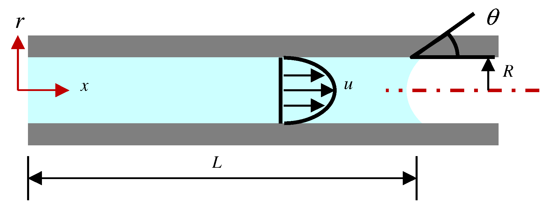
Figure 1 shows the schematic of the capillary-driven micro flow through a circular tube. For a Newtonian viscous liquid, if flow is laminar and incompressible, the governing equation for the unsteady flow velocity u(r, t) can be written as follows:

$$\frac{\partial u}{\partial t}=-\frac{1}{\rho }\frac{\partial p}{\partial x}+\frac{\mu }{\rho }\frac{1}{r}\frac{\partial }{\partial r}\left(r\frac{\partial u}{\partial r}\right)$$

(1)

where p is the pressure inside the tube, μ is the fluid viscosity, and ρ is the density. From the Laplace–Young equation, the driving capillary force at the meniscus is $2\sigma \cos \theta /R$, where σ is the surface tension coefficient, θ(t) is the dynamic contact angle, and R is the tube radius. The pressure gradient inside the tube is assumed to be linear and the fully developed laminar velocity profile can be used.

$$-\frac{dp}{dx}=\frac{1}{L(t)}\frac{2\sigma \cos \theta }{R}$$

(2)

$$u(r,t)=2L^{\prime }(t)\left(1-\frac{r^2}{R^2}\right)$$

(3)

where L(t) is the wetting distance at time t. In most previous approaches, the transient term $\partial u/\partial t=L^{″}$ is neglected. By substituting Equations (2) and (3) for Equation (1), an ordinary differential equation for the wetting distance is given as follows:

$$\frac{8\mu L}{\rho R^2}{L}^{\prime }-\frac{2\sigma \cos \theta (t)}{\rho R}=0$$

(4)

If the contact angle is assumed to be constant as a static contact angle θ_s, the solution for the wetting distance is the well-known Washburn equation [4].

$$\mathrm{Washburn} \mathrm{model}: L=\sqrt{\frac{2R\sigma \cos {\theta }_s}{4\mu }t}$$

(5)

Meanwhile, Ichikawa and Satoda [15] analyzed the interface dynamics of capillary flow in a tube considering inertial acceleration at the inlet of the tube and energy dissipation just after the meniscus. The dynamic balance of force in a horizontal tube is described as

$$\left(L+l\right)L^{″}+\frac{m}{2}{\left(L^{\prime }\right)}^2+\frac{8\mu L}{\rho R^2}{L}^{\prime }-\frac{2\sigma \cos \theta }{\rho R}=0$$

(6)

where l and m are correction factors for the inertial force and energy dissipation, respectively. The first and second terms in Equation (6) represent the inertial forces by tube entrance and liquid velocity itself, respectively. The third term is viscous force, and the fourth term is capillary force. Batten [18] assumed the values of l = 7R/6 from the inertial force in a hemispherical region of the tube inlet and m = 3.41 from an empirical relation. There is no analytic solution for Equation (6), but it can be solved numerically using the Runge–Kutta method by considering the dynamic variation of contact angle.

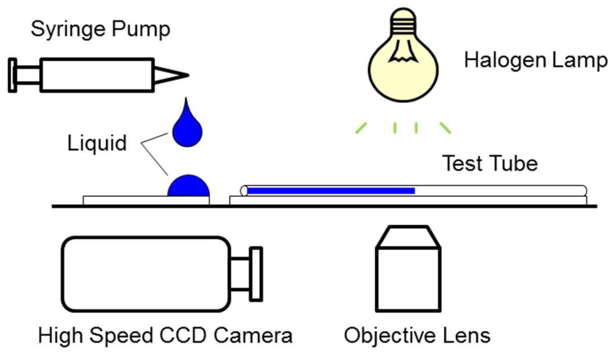
3. Experimental Apparatus

Figure 2 shows the schematic of the experimental setup. A drop of liquid is dispensed at the edge of a glass plate by a syringe pump, and then the glass plate is attached to a capillary tube in order to fill the liquid in by only the capillary force. The motion of the flow meniscus is observed using a fluorescence microscope (Nikon, Eclipse Ti, Tokyo, Japan) with a 4× objective lens. A halogen lamp is used as an illuminating light source and a high-speed CCD camera (SVSI) captures the images. The capillary tube is made of borosilicate glass with an inner diameter of 200 μm. The tube diameter is selected considering the typical gap height of the underfill process by capillary force in flip chip packaging. Careful attention was paid to tube cleaning because dust on the surface can distort the contact angle, or the wet surface can alter the interfacial force. In the cleaning process, the tube was kept immersed in water for six hours and then in a mixture of ammonium hydroxide, hydrogen peroxide, and water for one hour. Again, it was immersed in water for more than 24 h. Finally, it was dried in an electrolysis desiccator for 24 h. By changing the volume fraction of the glycerin–water mixture, the viscosity of the operating liquid is controlled. A small amount of water added to the mixture significantly changes the viscosity of the mixture. In the present study, the volume fractions of glycerin are 85.7%, 93.75%, 96.87%, and 99% at room temperature 20 °C, which yields the viscosity to be μ = 0.21, 0.54, 0.82, and 1.36 Pa∙s, respectively. The viscosity was measured by a rheometer (Brookfield DVIII + ULTRA). However, the fluid density ρ and surface tension coefficient σ are not sensitive to the small amount of added water [19,20]. Thus, ρ = 1260 kg/m³ and σ = 0.063 N/m are used for all the glycerin–water mixtures.

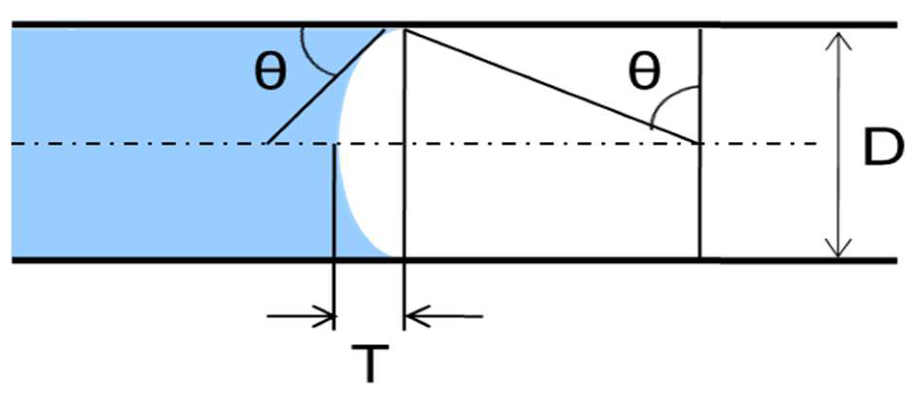
In order to measure the dynamic contact angle, the thickness T of the shadow image of the flow meniscus is obtained as shown in Figure 3. If the interfacial shape is assumed to be a part of a circle, the contact angle θ can be calculated by $\theta =2{\tan }^{-1}\left(0.5D/T\right)-\pi /2$ [21]. The spatial resolution for the contact angle measurement is enhanced by a high magnification microscope. The scale factor in image plane is 3.0 μm/pixel. The static equilibrium contact angle θ_s is evaluated from the image when there is no fluid motion.

Table 1. Static equilibrium contact angles and viscosities for various glycerin–water mixtures.

Volume Fraction of Glycerin (%)	Static Equilibrium Contact Angle (°)	Viscosity (Pa·s)
87.5	7.95°	0.21
93.75	7.98°	0.54
96.87	8.45°	0.82
99.0	8.95°	1.36

shows the values measured in this experiment. The dynamic contact angle, however, varies during the meniscus movement. The measurement length of the micro tube is 0–10 mm, so that the CCD camera cannot capture the whole field of view at one time. Thus, the measurement length is divided into three sub-sections, and then their data are combined successively. During the experiments, the tube inlet and the end of the camera screen are aligned on the same line after positioning the tube on the stage. Then, images are captured by incrementally moving the stages at intervals of 3.5 mm using a micro-axis transfer device. For each case, five experiments are conducted to obtain an average value. Since the interface movement depends on surface condition, all tubes are washed and dried for several hours. The careful cleaning of the tube surface assures the convergence of experimental data.

4. Results and Discussion

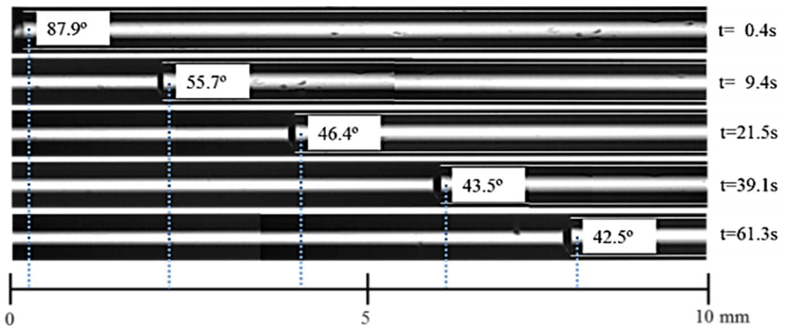
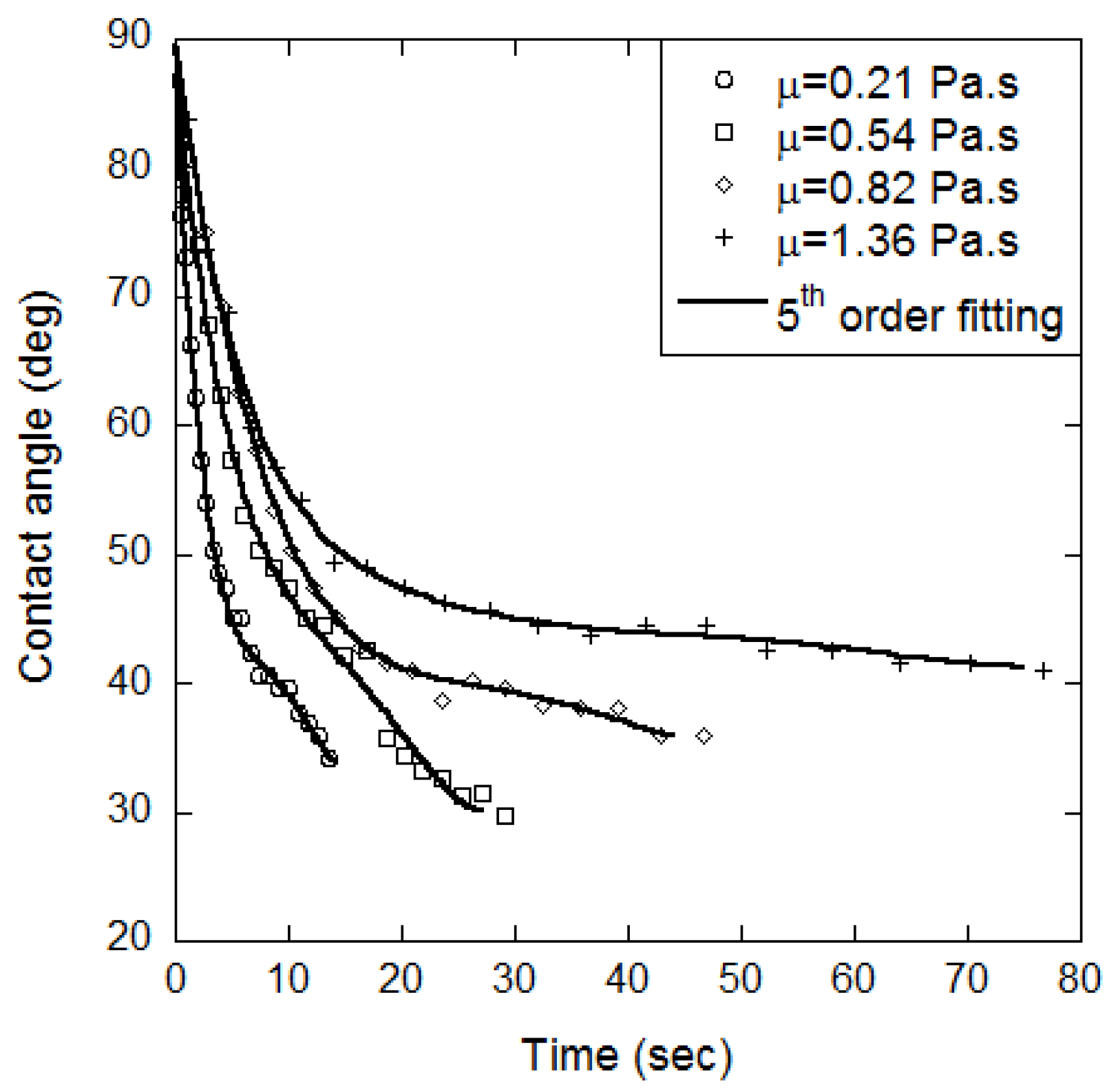
In Figure 4, the movement of the flow meniscus in the unsteady capillary flow is visualized for the whole measurement length in the case of a 99% glycerin–water mixture. In the visualization images, the meniscus has a maximum width of 174 pixels and a maximum thickness of 37 pixels. When the meniscus lies at the entrance region, the contact angle is nearly 90°, but it gradually decreases as the flow goes on. In many studies, approximate equations were developed for dynamic contact angles, such as empirical equations and the function of exponential. However, any of these equations do not have a perfect form for the decaying rate as time goes on. To minimize error, in the present study, the dynamic contact angle was determined by a polynomial equation with the least-square fitting method. Based on the visualized images in Figure 4, the variations of contact angle for all fluid viscosities are plotted in Figure 5. Here, the symbols denote the experimental data. The solid lines are least-squares fitted data to a polynomial function, respectively. The present data indicate that it approaches 90° at t = 0, and then it decreases according to the time until it reaches an equilibrium value. The higher viscosity of the liquid takes more time to reach the equilibrium contact angle.

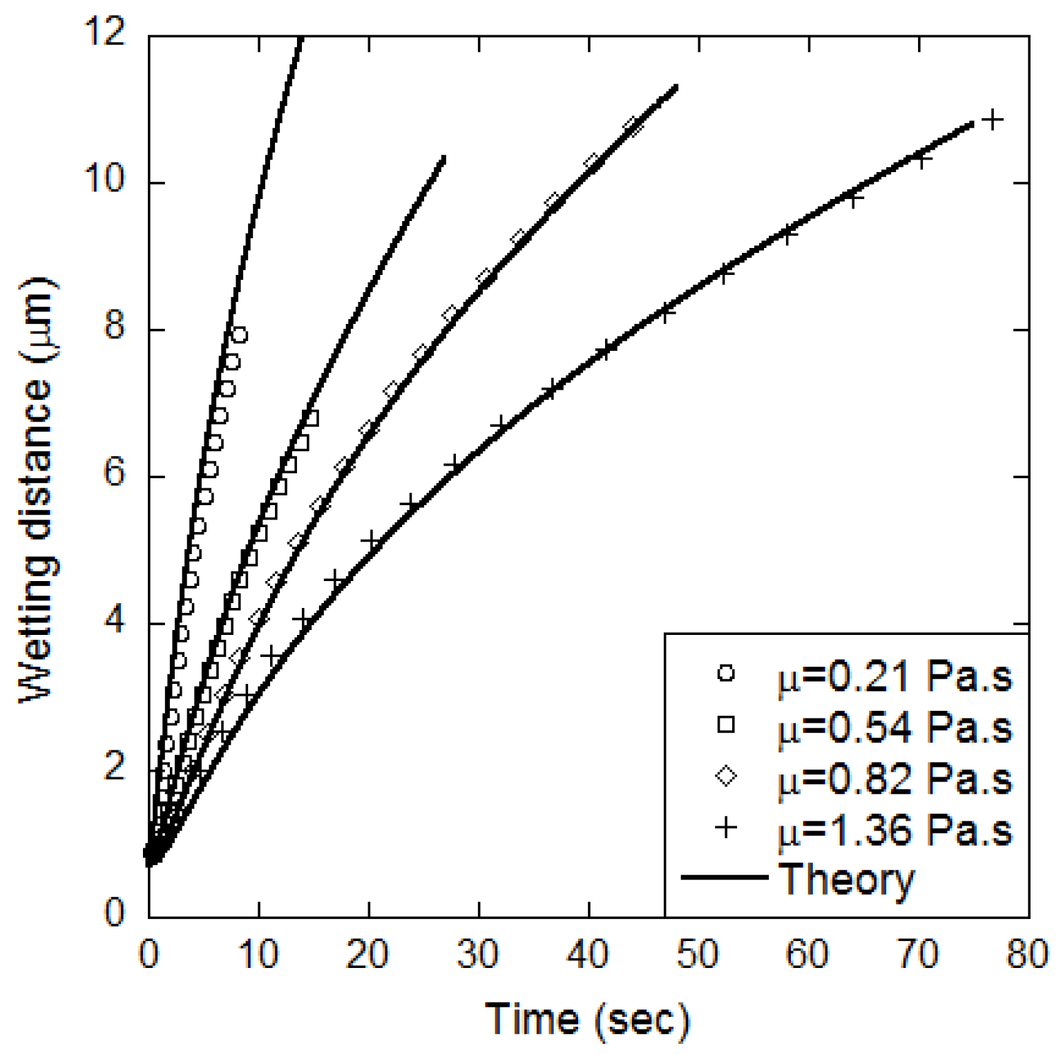
Figure 6 shows the wetting distances for various viscosities as a function of the filling time of the capillary meniscus. The measured data are averaged by five experiments in each case. The measured initial length is 700 μm from the inlet of the tube, and this initial length is also taken into account in the theoretical calculation. The overall patterns of wetting distance show that the meniscus moves fast just after fluid is dispensed at the edge, and then its traveling speed becomes slow. As the viscosity decreases, it takes more time for the meniscus to travel a given wetting distance. Theoretically, due to the viscous force acting as a resistance of the capillary flow, the fluid with a higher viscosity takes a shorter time to travel the same distance.

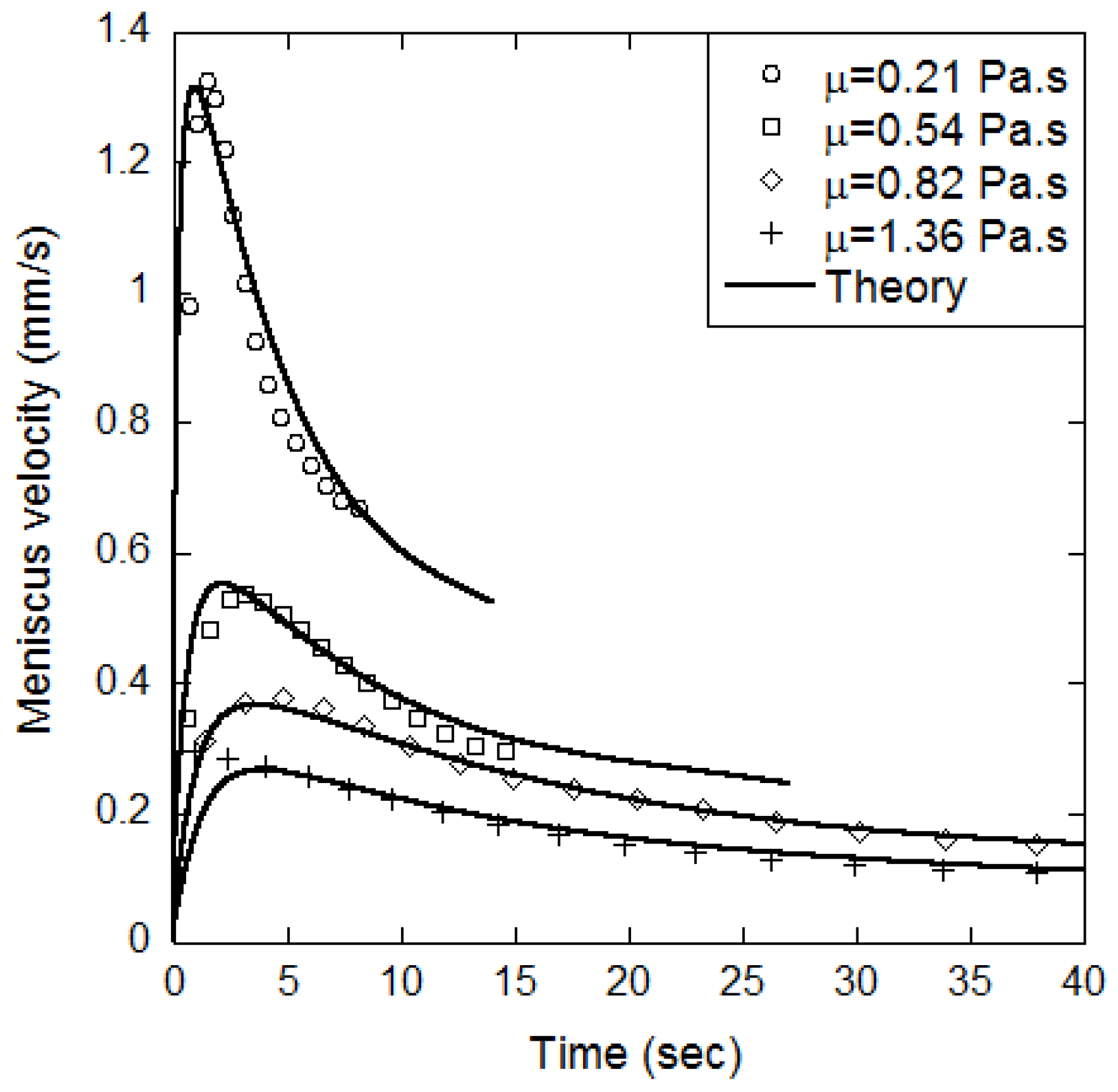
From the movement of the meniscus position in Figure 6, the meniscus velocity can be obtained by differentiating the meniscus position with time as shown in Figure 7. The velocity is very high at the entrance region, and then it decreases gradually. As the viscosity becomes lower, this results in higher velocity and a higher decreasing rate. Despite such a drastic change in the initial velocity, the theoretical data by Equation (6) agree well with experimental data. This agreement results from the consideration of all force terms acting on the capillary flow. However, it is still unknown which force is dominant in the flow. Thus, it is necessary to investigate the variation of each force in Equation (6) separately and search for the dominant force in capillary flow.

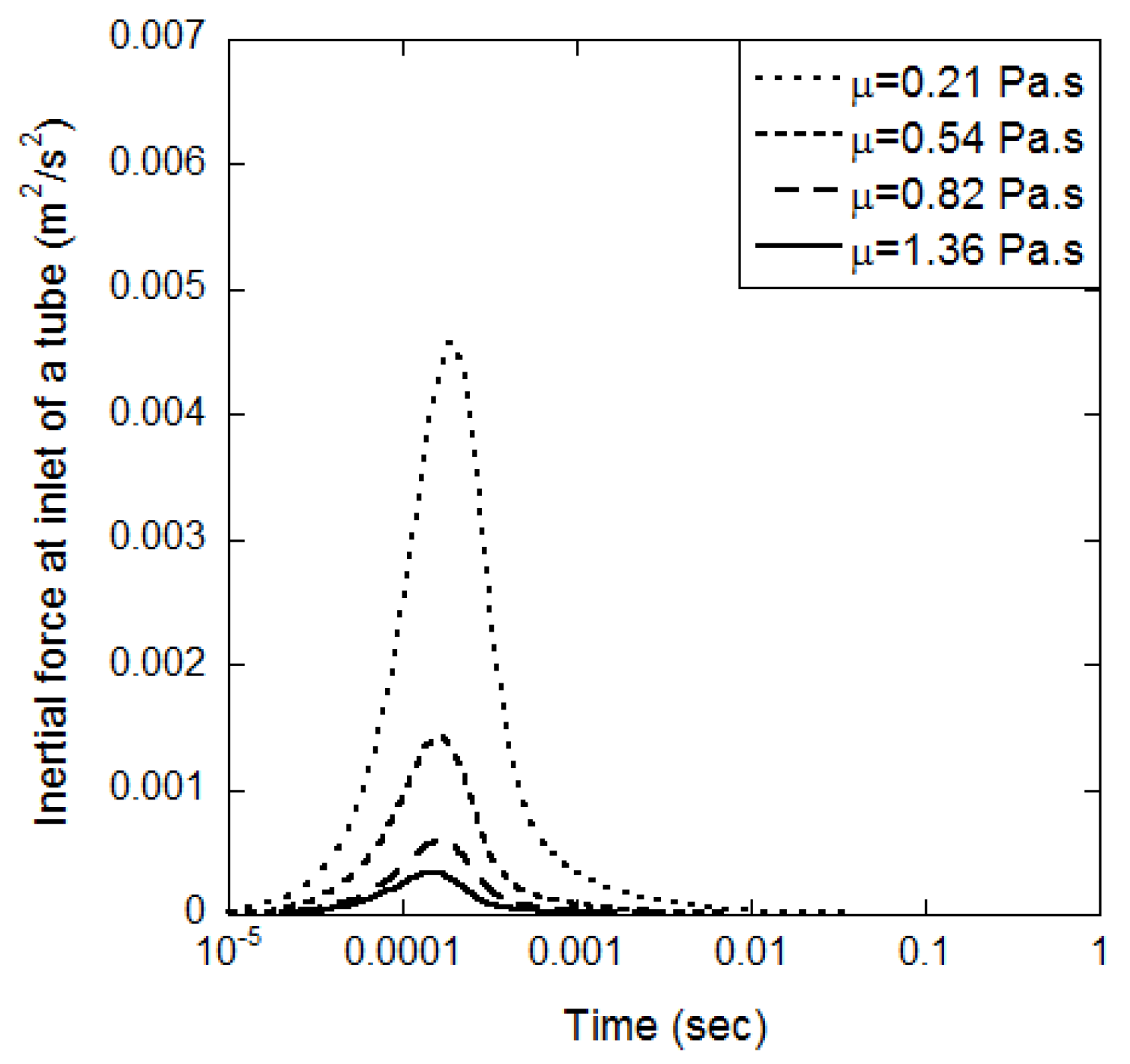
Figure 8 shows the inertial force at the inlet of the tube for various viscosities according to the time on a log scale. The inertial force starts from zero at the entrance of the tube and increases until it becomes maximum. Then, it decreases to zero within a short time. Since this force is a function of velocity, the force with the lower viscosity has the higher peak value. Szekely et al. [22] showed that the largest irreversible energy dissipation occurs through the formation of a vena contracta at the inlet of the tube. Batten [18] proved it by considering circular flow below the meniscus. On the other hand, in the present study, the magnitude of this force is very small compared with the other forces, so it does not have a significant impact on the overall flow. However, one should keep in mind that the force becoming larger at lower viscosity could not be neglected.

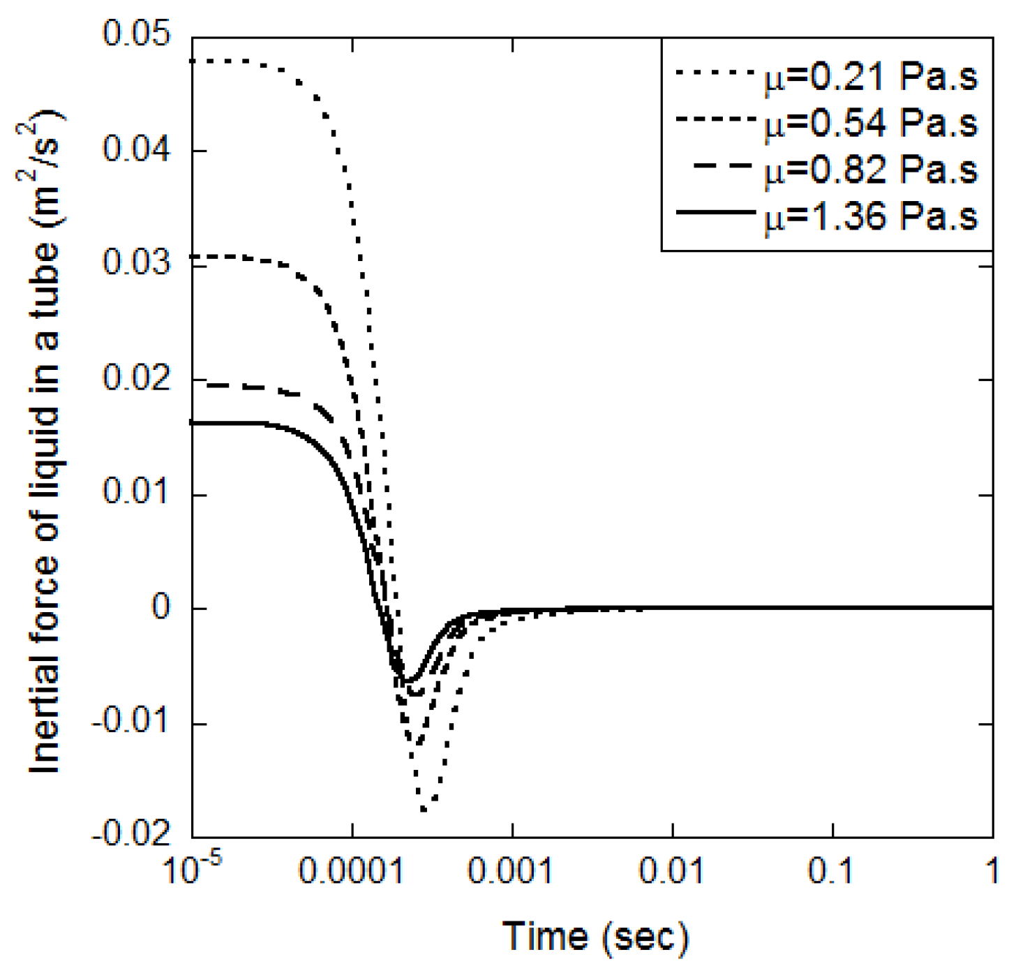
Figure 9 shows the variation of inertial forces of liquid in a tube with various viscosities according to the time. The highest inertial force is observed immediately after the fluid is attached at the inlet of the tube, and it sharply decreases until the minimum value. There is a temporary negative value of inertial force due to the sharp decreasing rate and the magnitude is larger at a lower viscosity. The negative inertial force is close to zero thereafter, and its magnitude is kept constant. It is also the same trend as the meniscus acceleration due to this force as a function of acceleration term. Based on the effect of inertial force by viscosity, the Washburn model [4], which neglects the inertial force, can be suitable for the high viscous fluid; however, inertial force significantly impacts the capillary flow.

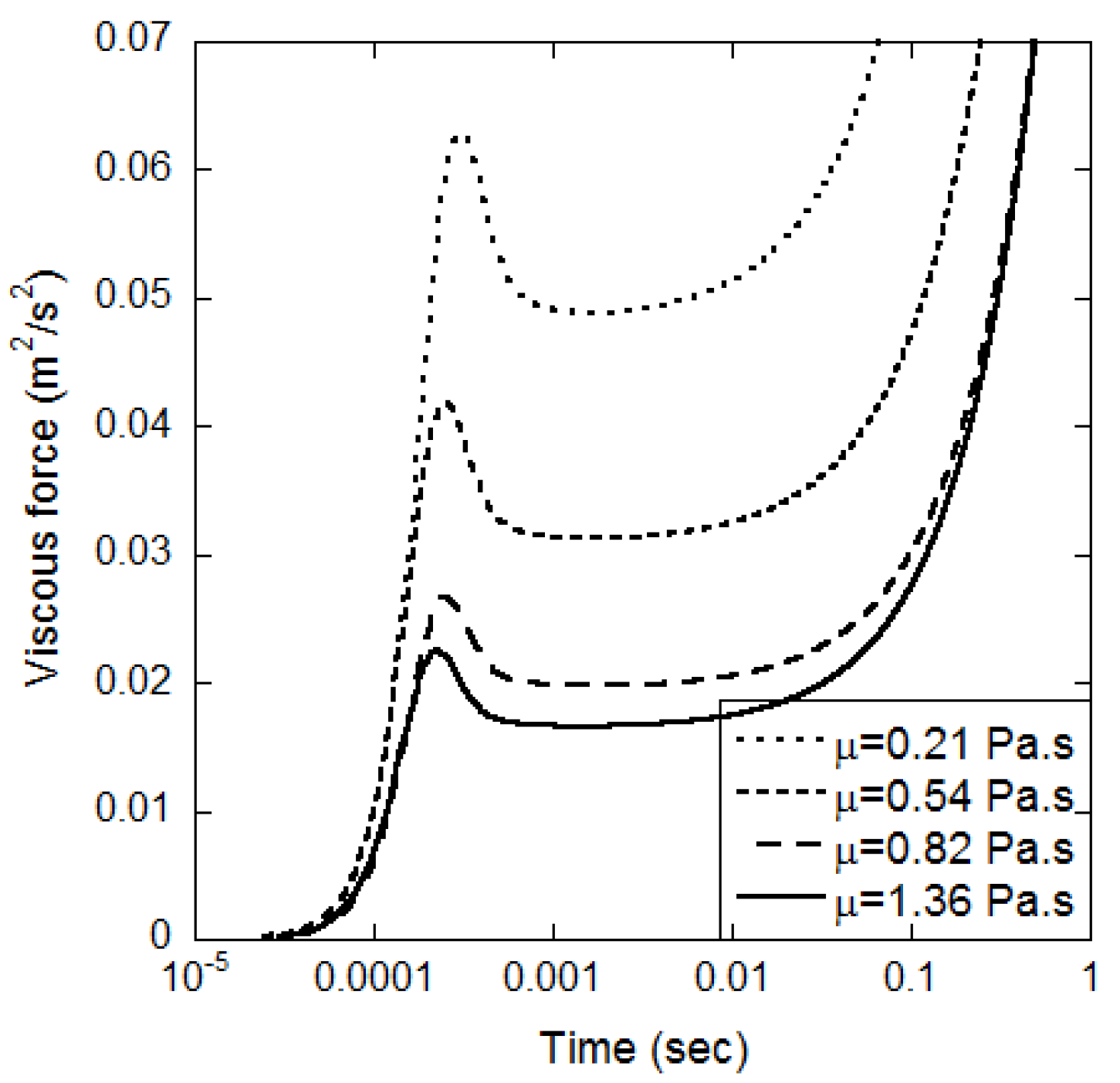
Figure 10 shows the variation of viscous forces of liquid in a tube with various viscosities according to the time. The lower viscosity has the larger viscous force, and it seems like a reverse trend of the inertial force. A faster fluid velocity by increasing inertial force causes increasing frictional resistance against a surrounding wall. Thus, the viscous force represented by the resistance within the fluid depends on the inertial force acting on the acceleration of the fluid.

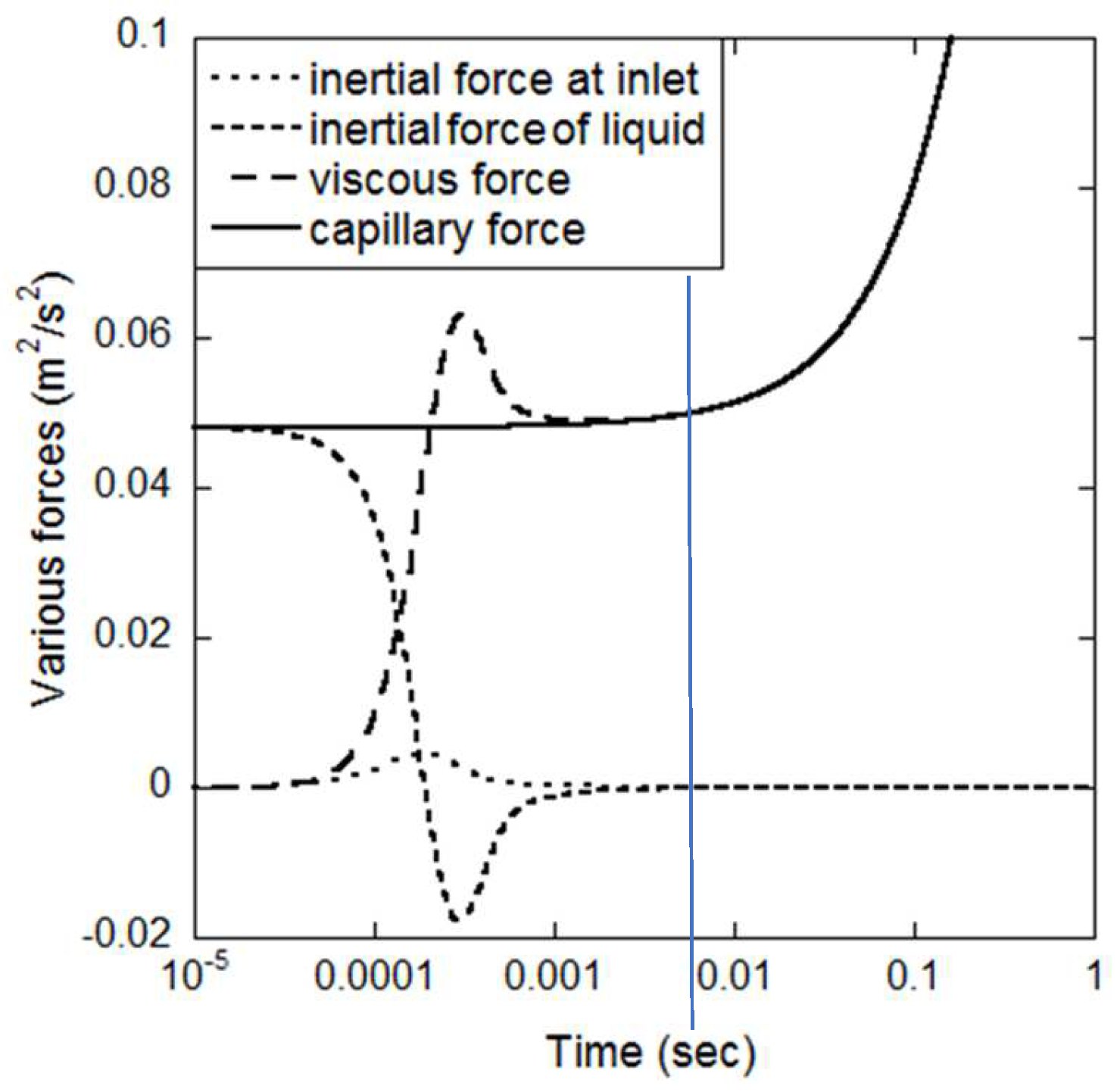
Figure 11 shows that the momentum balance of four forces is concerned with capillary flow. To magnify the initial regime, the time axial has a range up to 0.001 s, in which capillary force is equal to the viscous force. At the beginning (t = 0), there is a decrease in the inertial force of liquid in a tube and an increase in viscous force after the viscous force becomes dominant over the inertial force. The velocity is at maximum at 0.0002 s, and it is at this point where the inertial force at the inlet of a tube is at maximum. Thereafter, since the inertial forces of the two types are reduced close to zero, the forces acting on the fluid become gradually trivial. Meanwhile, the capillary force is equal to the sum of the overall force acting on the fluid. Hence, it is equal to the inertial force at first time; after time, it is equal to the viscous force. Even if the viscous force increases after the maximum velocity, the capillary force by influence of dynamic contact angle also increases. This is the reason why the velocity of actual capillary flow has declined very slowly.

Fries and Dreyer [23] provided a method to determine a dominant region divided into three stages, such as the purely inertial, viscous–inertial, and purely viscous stages. To separate the stages, the times calculated by Quere [7], Bosanquet [6], and Washburn’s equation [4] are defined as 3% deviation criteria computed result. In a similar method, the present study’s time stages were separated by momentum previously calculated, and the formulas are given as follows:

$$\begin{gathered} \mathrm{Purely} \mathrm{inertial} \mathrm{time} \mathrm{stage} \\ \hspace{1em}\hspace{1em}\hspace{1em}\hspace{1em} \frac{inertial-viscous}{capillary}=0.97 \end{gathered}$$

(7)

$$\begin{gathered} \mathrm{Viscous}–\mathrm{inertial} \mathrm{time} \mathrm{stage} \\ \frac{viscous-inertial}{capillary}=0.97 \end{gathered}$$

(8)

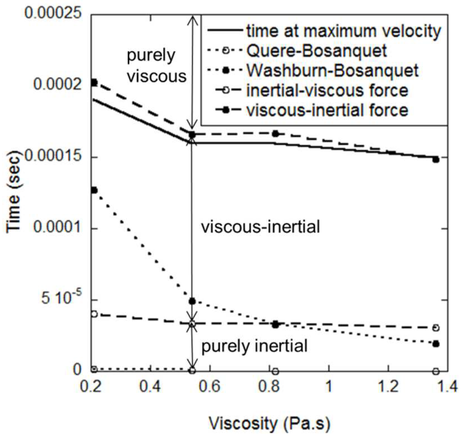
Figure 12 shows the times for the dominant momentum according to the various viscosities in comparison with Fries’ approach [23]. As viscosity lowers, the interval between two different approaches is greater, but overall initial time becomes shorter at a higher viscosity. This result brings to mind that the capillary force varying with dynamic contact angle plays an important role in determining the maximum velocity. Due to assuming a constant contact angle, the constant capillary force caused high initial velocity in a short time, and it slowed down fairly fast. However, rapidly changing velocity within a short time does not occur in actual flow; thus, a wider time interval for the present approach is closer to the actual flow. As proof of this, the time at maximum velocity exists in the viscous–inertial region as positive acceleration, but it is not included in the purely viscous region as negative acceleration.

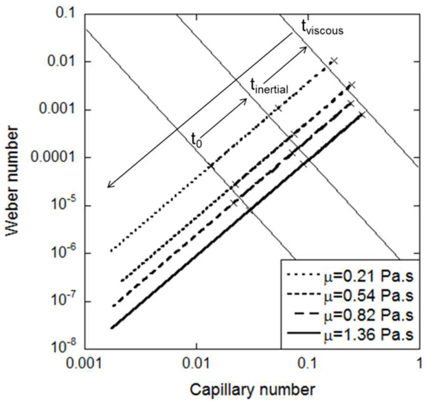
In order to compare the magnitude of interfacial force, inertial force, and viscous force, Hoffman [9] used the dimensionless numbers with regard to the capillary flows, such as the capillary number (Ca = μV/σ) and Weber number (We = 2ρVL/σ). In the same way, Figure 13 shows the magnitude of three forces for various viscosities as a function of the dimensionless number. It is found that the data lines are overlapped in a certain interval, which is separated by three asymptotic lines obtained from time stages [8,9]. In the plot, the capillary number and Weber number rapidly increase and reach maximum until the viscous–inertial regime (t₀ < t < t_viscous), but the numbers continually decrease after that until the end of the process (t > t_viscous). This is the same manner with meniscus velocity due to the dimensionless number as a function of velocity. In terms of dominant force, at low capillary and Weber numbers, the interfacial force is absolutely dominant, which agrees with the result of Hoffman’s review table [9]. In addition, there exists only the inertial force as the dominant force at purely inertial regime (t₀ < t < t_inertial), and the viscous forces are significantly increased at viscous–inertial regime (t_inertial < t < t_viscous), where inertial and viscous forces exist as dominant forces but proceed in opposite directions. Thus, lower viscosity increases inertial force, and higher viscosity increases interfacial and viscous forces.

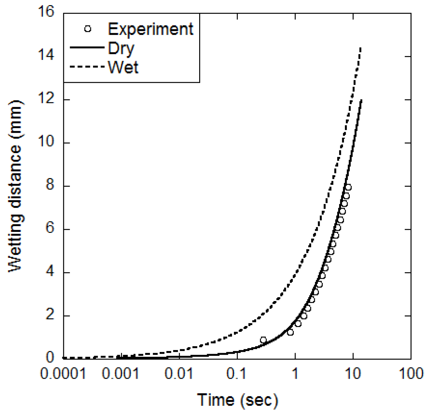
The capillary force determines the balance of other forces, and it has various parameters, such as density, surface tension, and contact angle. If variations of density and surface tension are neglected, the capillary force varies with the contact angle from the equations. The contact angle depends on the surface conditions inside the tube, which causes a considerable problem in liquid penetration tests. Ichigawa’s experiment [15] has two different conditions, in which the surfaces of the inner tube are dry or wet. In their study, the result showed that the experimental data for the wet condition agrees quite well with the theory. However, in Figure 14, the experimental data are found to be similar to the dry condition rather than the wet condition. This result comes from the consideration of the dynamic contact angle. Generally, if the contact angle is ignored or considered as a static contact angle, its value is calculated using a 0° or fixed equilibrium value. This assumption corresponds to the wet conditions due to covering with liquid of the inner surface. On the other hand, if the condition of the inner surface is completely dry, and theoretical data are considered the time-varying dynamic contact angle from 90 to the equilibrium value, it corresponds to the flow of the fluid in the dry condition. Thus, in this plot, it is found that the experimental data for dry conditions agree well with the theoretical data that considered dynamic contact angle.

5. Conclusions

The present study investigated the dynamic behavior of the micro capillary flow in a circular tube. The wetting distance, dynamic contact angle, and meniscus velocity have been measured for liquids with different viscosities using a microscope. The analytical model is calculated with the estimated physical properties and function of the dynamic contact angle. By comparing the experimental data with the analytical data, the model fits well with experimental data as the fluid with a lower viscosity has a faster velocity. In other words, as the viscosity decreases, it takes less time for the meniscus to move a given wetting distance. Based on the model, the momentum balance of four forces is concerned with capillary flow. Here, the capillary force increases as time goes on; the inertial and viscous forces corresponding to the capillary force have reversed trends. Furthermore, in order to determine which time section is dominant, the time is separated by dominant forces. As a result, the time stage with a lower viscosity is longer than the others. By using these time stages, the magnitudes of the forces according to the dimensionless number were compared. As a result, lower viscosity increases inertial force, and higher viscosity increases interfacial and viscous forces. Finally, the surface condition with regard to the interfacial force is completely dry, and the analytical data agree well with the experimental results.