Abstract
Considering that the choice of loss function plays a significant role in the derivation of Bayesian estimators, we propose a novel asymmetric loss function named the weighted Q-symmetric entropy loss for computing the estimates of the parameter and reliability function of the Burr XII distribution. This paper covers the classical maximum-likelihood, uniformly minimum-variance unbiased, and Bayesian estimation methods under the squared error loss, general entropy loss, Q-symmetric entropy loss, and new loss functions. Through Monte Carlo simulation, the respective performances of the considered estimators for the reliability function are evaluated, indicating that the Bayesian estimator under the new loss function is more efficient than those under other loss functions. Finally, a real data set is used to demonstrate the practicality of the presented estimators.
1. Introduction
A system’s reliability function, , represents the probability that an object survives longer than time t, which is also called the survival function. Reliability analyses are mainly devoted to forecasting the probability of survival time for experimental systems, which can help administrators control costs, plan maintenance actions, and assess system availability. Based on the needs of practical applications, numerous scholars have investigated the reliability of different distributions, making use of classical estimators and Bayesian estimators under various loss functions and different priors. The authors of [1] provided the maximum-likelihood and Bayesian estimates for the three-parameter exponential–Weibull distribution with type-II censored samples. The authors of [2] analyzed the parameter estimates and reliability features of the one-parameter Lindley distribution using classical and Bayesian techniques with progressive type-II censored samples. A novel parameter estimation method named the E-Bayesian method was introduced in [3], which was used to estimate the reliability under a binomial distribution. Under a hybrid model with two exponential distributions of certain mixing proportions, the authors of [4] investigated the unbiased estimations of the reliability function. Furthermore, the equivalent unbiased estimators of the reliability were also derived under the scenario where the negative weighting of the components of the mixture distribution was allowed. The authors of [5] considered an estimator of the reliability function of the power Lomax distribution in stress–strength models. The authors of [6] obtained the classical reliability estimations of a multi-component system, in which the stress and strength variables followed the unit-generalized exponential distributions. The Bayesian estimations with Gamma and weighted Lindley priors were also discussed. On account of the situation where the data of torpedo loading tests were limited and included samples without failures, the authors of [7] proposed a new Bayesian evaluation method based on fused information to estimate the reliability of torpedo loading, for which the lifetime distribution and failure rate prior distribution were assumed to follow exponential and Gamma distributions, respectively. The authors of [8] calculated the estimators of the reliability for the adaptive, type-II progressive censored data of the unit-Lindley distribution using frequentist and Bayesian methods.
In contrast to the limitations of classical estimation methods, which exclude prior information, Bayesian estimates have been more abundantly researched by scholars in recent years due to their consideration of prior distributions, allowing for the inclusion of historical or subjective information. In Bayesian methods, estimates are obtained using different loss functions. Therefore, one of the main challenges for researchers is choosing the right loss functions according to the specific situation; that is, a well-designed loss function yields a more accurate Bayesian estimator. Many scholars have investigated new loss functions and compared the performance of Bayesian estimators under different loss functions. The authors of [9] discussed the Bayesian parameter estimator of the Lindley distribution and their corresponding posterior risks separately using seven different loss functions. However, in response to the derivation error of the posterior risks under the entropy loss function in the paper, a correct derivation was given in [10]. The authors of [11] proposed a novel analysis method to evaluate potential loss in a process safety field. The potential loss analysis was discussed in detail along with case studies. The authors of [12] suggested defining a new loss function for use in Bayesian methods to decrease the effects of outliers in crowd behavior analysis. The authors of [13] proposed a novel loss function named the weighted composite Linex loss function and compared the performance of the estimators under it with other estimators under the Linex loss, weighted Linex loss, and composite Linex loss functions. The authors of [14] introduced a novel weighted general entropy loss function and compared it with other loss functions. The authors of [15] derived the parameter estimations of the exponential distribution with complete data, which were comparatively analyzed using maximum-likelihood and Bayesian estimations with the squared error loss, entropy loss, and composite Linex loss functions.
The Burr XII distribution is very flexible as a lifetime distribution, as its hazard rate function can be either monotonic or unimodal, which means that it is much more suitable for modeling different types of lifetime data. Thus, it is more compatible with the precise situations of system reliability analysis and has been widely studied by scholars and applied in practice.
The probability density function (PDF) and cumulative distribution functions are expressed as
where and represent the shape parameters.
The hazard rate and reliability functions are expressed as
As a vitally flexible distribution, the Burr XII distribution has many tight connections with other well-known distributions. When , , and , the Burr XII distribution is equivalent to the Pareto, log-logistic, and paralogistic distributions, respectively, with all their scale parameters equal to 1.
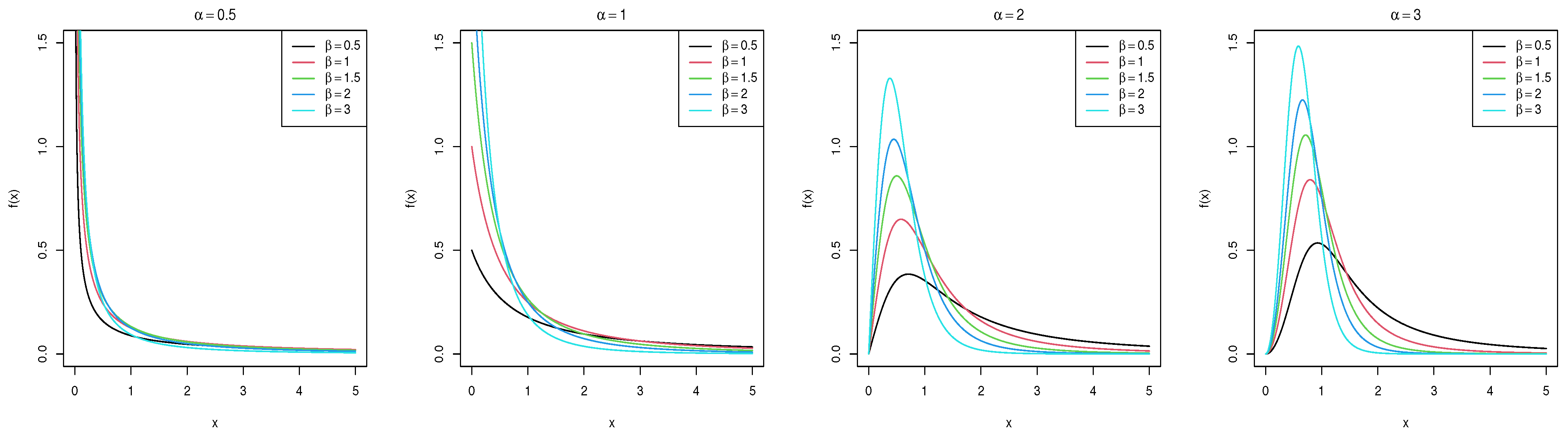
The PDF plots corresponding to the selected parameter values are shown in Figure 1.
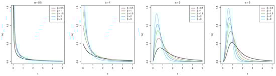
Figure 1.
PDF plots of the Burr XII distribution for varying parameter values.
Based on Figure 1, when , the PDF plots of the Burr XII distribution have a single peak, which is skewed to the right. As increases, the density plot becomes steeper. In contrast to the case of , the function curve monotonically decreases when .
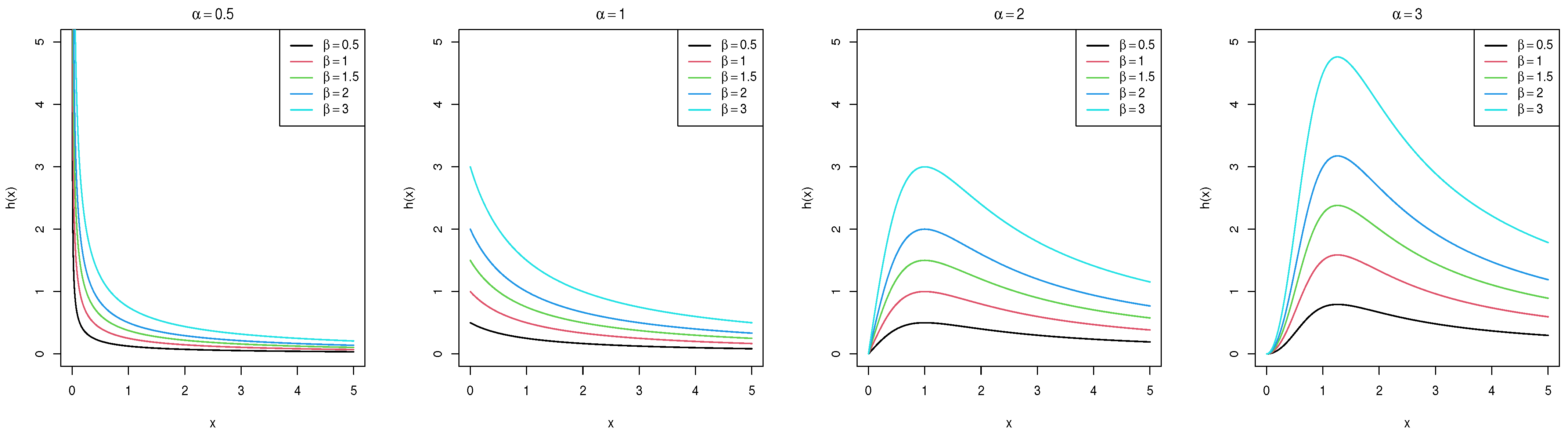
The hazard rate plots with different values of are shown in Figure 2, indicating that the hazard rate decreases monotonically for . However, when , the hazard rate quickly reaches its peak and then decreases as the argument x increases. As x approaches ∞, the hazard rate value converges to a constant value. Moreover, the hazard rate has higher values when is larger.
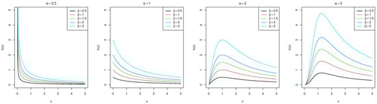
Figure 2.
Hazard rate plots of the Burr XII distribution with different values of .
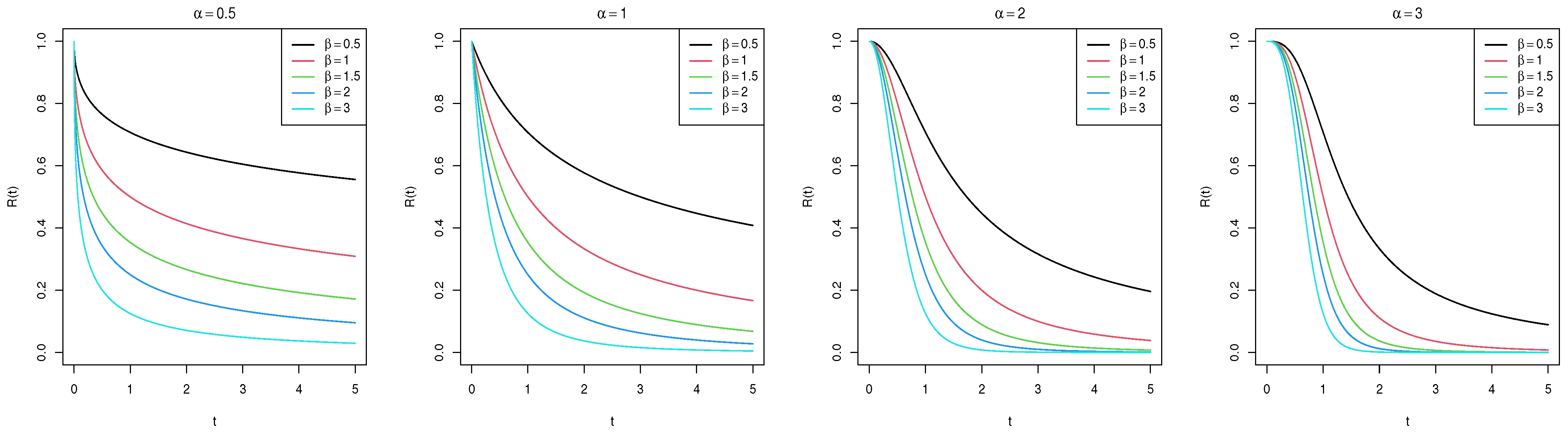
The reliability plots are shown in Figure 3.
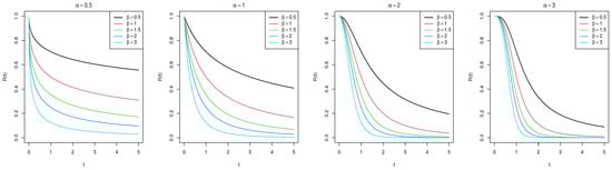
Figure 3.
Reliability plots of the Burr XII distribution with different values of .
The Burr XII distribution has a broad range of applications in lifetime analysis due to its excellent flexibility and practicality as a lifetime distribution. The Burr XII distribution was adopted in [16] to investigate the reliability of a transit traffic control system with medium loads. Using a progressive type-II censored scheme, the authors of [17] considered estimates for the Burr XII distribution using E-Bayesian methods. The authors of [18] discussed the Bayesian estimators of the parameters and reliability under the Burr XII distribution, which were compared with classical maximum-likelihood estimation. For a mixture system of three Burr XII distributions, the authors of [19] analyzed the Bayesian and maximum-likelihood estimators, along with the elegant closed-form algebraic expressions of Bayesian estimators, as well as the posterior risks. Under the Burr XII distribution, the authors of [20] introduced an improved adaptive type-II progressive censoring scheme, in which the frequentist and Bayesian inferences were established.
Concentrating on the Burr XII distribution, this study covers the maximum-likelihood estimation (MLE), uniformly minimum-variance unbiased estimation (UMVUE), and Bayesian estimations of the shape parameter and the reliability function. For Bayesian estimations, the squared error loss (SEL), general entropy loss (GEL), and Q-symmetric entropy loss (QEL) functions, together with the new loss function proposed in this paper named the weighted Q-symmetric entropy loss (WQEL), were applied. Our innovation lies in providing UMVUE and Bayesian estimations under the new loss function for the reliability of the Burr XII distribution. The evaluation of the given estimators, especially the Bayesian estimators under the new WQEL function, is also discussed.
The remainder of this paper is structured as follows. In Section 2, the frequentist methods of the MLE and UMVUE under the Burr XII distribution are investigated. Section 3 deals with the Bayesian estimators under the three pre-existing loss functions, namely the SEL, GEL, and QEL functions. In Section 4, a novel loss function named the weighted Q-symmetric entropy loss function is proposed and applied. The Monte Carlo simulation is established in Section 5, which is conducted to assess the performance of the given estimators. In Section 6, a remission time data set is used to demonstrate the utility of the discussed estimators.
2. The Classical Estimators of the Parameters and Reliability
In this section, we focus on the calculation of the classical estimators, including the MLE and UMVUE, for both the parameter and the reliability function.
2.1. Maximum-Likelihood Estimation
Let denote a sample of size n from the Burr XII distribution; therefore, the likelihood function is computed as
and the log-likelihood function is
Consequently, the derivative of Function (6) concerning is
The second-order derivative of Function (6) is expressed as
which means that exists and is unique.
We set Function (7) to zero in order to find the value of that maximizes Function (6), which is also the MLE of . It is obtained as follows:
where is supposed to be known.
According to the unique invariance property of the MLE, is naturally computed as
2.2. Uniformly Minimum-Variance Unbiased Estimation
Suppose that represents a random sample of the Burr XII distribution. Then, the statistic has a distribution, for which the PDF is structured as follows:
where denotes the Gamma function.
The statistic S can be proved to be a sufficiently complete statistic for . According to the Lehmann–Scheffé theorem, given , the UMVUE of the parameter is
and the approximate UMVUE expression of is
In order to obtain an accurate expression for the UMVUE of , we present the following theorems.
Theorem 1.
When considering the random sample from the Burr XII distribution, the UMVUE of the PDF at a given point, x, is expressed as
where .
Proof.
Based on the Lehmann–Scheffé theorem, as S is a completely sufficient statistic, we can infer that , which is the conditional PDF of given S, is the UMVUE of .
Let L denote , for which the PDF is structured as
where .
Then, considering the independence between L and , the joint PDF of L and is written as .
As , we perform a variable transformation to obtain the joint PDF of , which is
Additionally, the PDF of S is
Thus, the conditional PDF of given S is obtained as . That is, the UMVUE of is calculated as
□
Based on Theorem 1, the UMVUE of is presented in Theorem 2.
Theorem 2.
Given the estimate of the PDF , the UMVUE of the reliability function is derived as
Proof.
In order to prove the first equality of the theorem, we note that is the function of S, which is sufficient and complete for . Thus, we only need to prove that is unbiased for .
where denotes the PDF of S.
Then, we can calculate the specific expression for as follows:
□
3. Bayesian Estimation under the SEL, GEL, and QEL Functions
The choice of loss function is an essential element of Bayesian methods. In this section, we first compute the Bayesian estimators under three commonly applied loss functions, including the squared error loss (SEL), general entropy loss (GEL), and Q-symmetric entropy loss (QEL) functions, in order to compare the effects of the estimators under the newly proposed loss function.
Suppose is the estimate for the parameter to be estimated. Then, the SEL, GEL, and QEL functions are defined as follows:
In order to evaluate the performance of different Bayesian estimators in multiple scenarios, we consider both informative and non-informative priors.
3.1. Bayesian Estimation under the Informative Prior
Assume that follows the informative Gamma prior distribution with the hyperparameters , which is expressed as
Therefore, the posterior distribution function of is
The Bayesian estimations of the parameter under the above loss functions are, respectively, computed as
Furthermore, the Bayesian estimations of under the SEL, GEL, and QEL functions are calculated separately as
3.2. Bayesian Estimation under the Non-Informative Prior
The non-informative prior utilized is the quasi-density prior. It has broad applications, such as its employment in [21] for the calculation of the Bayesian and Bayesian shrinkage estimators. The quasi-density prior of is defined as
Based on the quasi-density prior, the posterior distribution function follows . Due to the positivity of the hyperparameters of the Gamma distribution, it is important to ensure that is greater than 0. The Bayesian estimations of the parameter are given as
The Bayesian estimators of are expressed as follows
4. A Novel Loss Function: The Weighted Q-Symmetric Entropy Loss (WQEL) Function
Inspired by the weighted general entropy loss function introduced in [14], the proposed novel loss function, WQEL, is defined based on the QEL function. In this section, we present the definition and a brief description of the WQEL function. The relevant Bayesian estimators under it are also included.
4.1. The Definition of the WQEL Function
The WQEL function is derived from the QEL function and is defined as
where denotes the weighted function imposed on the expression of the QEL function. Obviously, the WQEL function is a generalized form of the QEL function, and it is asymmetric. When , the WQEL devolves into the QEL.
For symmetric loss functions, such as the QEL function, overestimates and underestimates have the same effects on its function value. Thus, the estimates obtained from the QEL are inaccurate in cases where there is a bias toward overestimated or underestimated values. In contrast to the symmetry of the QEL function, the new WQEL function is asymmetric, which means that it is more practical and flexible than the QEL function.
Specifically, when , the WQEL function degrades into the QEL function, the estimator of which has no preference for overestimation or underestimation. When , the estimator under the WQEL function is more biased toward the case of , and vice versa for the case of .
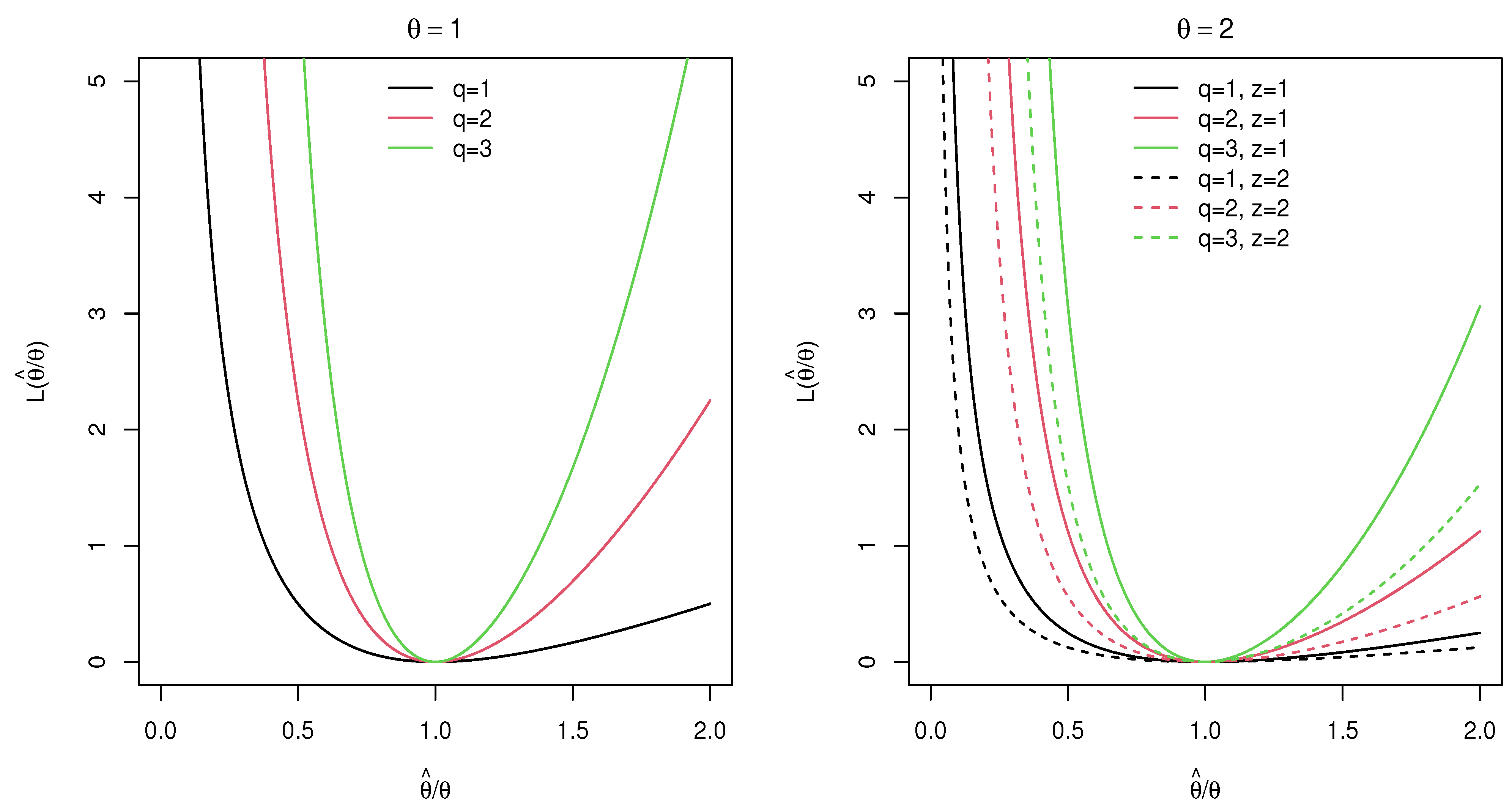
Figure 4 provides a graphical representation of the WQEL function with the given parameter values and the chosen values of q and z.
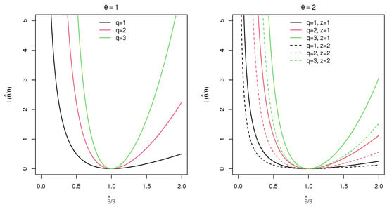
Figure 4.
The plots of the WQEL function.
From Figure 4, we can conclude that the WQEL function is strictly convex and non-negative. Moreover, regardless of the values of the parameters q and z, as the deviation of from 1 increases, the value of the WQEL function grows larger, fulfilling the requirements for a loss function. However, when , the WQEL is equivalent to the QEL function, which means that the value of z has no effect on the value of the WQEL function. Additionally, increasing the value of q or decreasing the value of z leads to a larger function value.
Theorem 3.
Under the WQEL function , the Bayesian estimate of θ to be estimated is derived as
Proof.
The Bayesian estimation for is the estimate used to minimize the posterior risk, which is expressed as
where refers to the given posterior distribution. Considering that the parameter estimate under the WQEL function aims to minimize the posterior risk, we find
It is worth clarifying that is a convex function; thus, we can straightforwardly obtain the minima of the posterior risk by setting . Consequently, the Bayesian estimation of under the WQEL function is
□
Moreover, it is worth mentioning that when and , the estimators under the WQEL function are equivalent to the estimators under the SEL function; that is, the WQEL function is an extension of the SEL function.
4.2. Bayesian Estimations under the WQEL Function
According to Theorem 3, the Bayesian estimator of under the informative Gamma prior distribution with the hyperparameters is given as
Furthermore, the reliability function’s Bayesian estimator for the Burr XII distribution is represented as follows:
Regarding the non-informative quasi-density prior, as , the Bayesian estimations of and under the new loss function are expressed separately as
5. Simulation
Monte Carlo simulation is widely employed in the literature to assess the performance of different models. For example, the authors of [22] employed it to estimate the reliability of logistics and supply chain networks. This section concentrates on a graphical demonstration of the performance under the applied reliability estimators for comparison and assessment purposes using Monte Carlo simulation. The simulation program was operated using the statistical software R, version 4.2.2. We conducted the simulation using a Windows 10 system with an 11th Gen Intel(R) Core(TM) i5-1135G7 @ 2.42 GHz CPU.
Different estimation methods were evaluated by comparing the mean squared error (MSE), which is defined as
where N represents the number of iterations.
Given that the acts on a given value t for , we then adopted the Mean Integrated Squared Error () to measure the performance of the discussed estimators for the reliability function globally. The is defined as
where refers to the particular values of t selected from the reliability function and T is the number of the selected values denoted by .
The simulation involved the following procedures:
- (1)
- Before proceeding with the simulation, we initially determined the values of each known parameter in the model. The parameters and appeared in the Burr XII distribution and were set as and . We employed sample sizes of and . In the Bayesian estimators, the hyperparameters of the informative Gamma prior were , and the values of m in the quasi-density prior were . As for the value p, which occurred in the GEL function, it was set as and . We considered for the QEL function, as well as and for the WQEL function. For the choice of , we aimed to verify that the WQEL estimator for was equivalent to the estimator under the SEL function. For the latter, it represented a choice of parameters for the WQEL estimator that exhibited the best performance, which we determined after many attempts.
- (2)
- We obtained n samples randomly selected from the Burr XII distribution using the inverse transforming sampling method with the given values of and .
- (3)
- We repeated step (2) times and calculated the values. When N was large enough, the effects of random errors occurring each time we obtained the random sample in step (2) diminished, resulting in more informative simulation results.
As observed in Figure 1, significant variations emerged with small values of t in the probability density plots. Thus, it should be noted that when computing the , we took the argument of the reliability function as . The simulation records are presented in Table 1, Table 2, Table 3, Table 4 and Table 5.

Table 1.
The MLE and UMVUE of , with their MSEs shown in brackets.
Table 2.
The Bayesian estimates under the SEL function and and , with their MSEs shown in brackets.
Table 3.
The Bayesian estimates under the GEL function and and , with their MSEs shown in brackets.
Table 4.
The Bayesian estimates under the QEL function and and , with their MSEs shown in brackets.
Table 5.
The Bayesian estimates under the WQEL function and and , with their MSEs shown in brackets.
The estimates were evaluated with varying values of , n, m, p, q, and z.
From the Monte Carlo simulation results, we can conclude the following:
- (1)
- By comparing Table 2, Table 3, Table 4 and Table 5, it is evident the estimators under the WQEL function for the parameter exceeded the estimators under other loss functions from a comprehensive point of view due to their smaller MISE values. This result is better visualized in Figure 5.
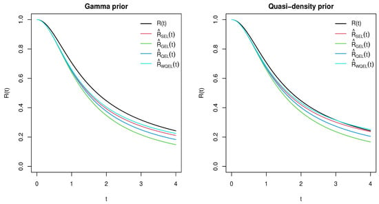 Figure 5. Plots of the Bayesian estimators under the SEL, GEL, QEL, and WQEL functions.
 - (2)
- Based on the results in Table 2 and Table 5, a Wilcoxon signed-rank test was conducted for the corresponding estimates under different priors in order to determine whether the estimates under the SEL and the WQEL with were significantly different. The null hypothesis for the test was that there was no significant difference between the two sets of data. The significance level was set at . Based on the results in Table 2 and Table 5, the p-value of the Wilcoxon signed-rank test was calculated as , indicating that the estimates under the SEL and WQEL function with had similar values. Thus, when , the estimators under the WQEL function were equivalent to those under the SEL function. This demonstrates the flexibility and advantages of the new WQEL function.
- (3)
- As seen in Table 1, the classical estimators under the Burr XII distribution with parameter were more efficient than the estimators when .
- (4)
- As seen in Table 2, Table 3, Table 4 and Table 5, regardless of the loss function used, the estimates under the informative Gamma prior were more efficient than those under the non-informative quasi-density prior, which demonstrates the benefit of an appropriate informative prior distribution for Bayesian estimators.
- (5)
- (6)
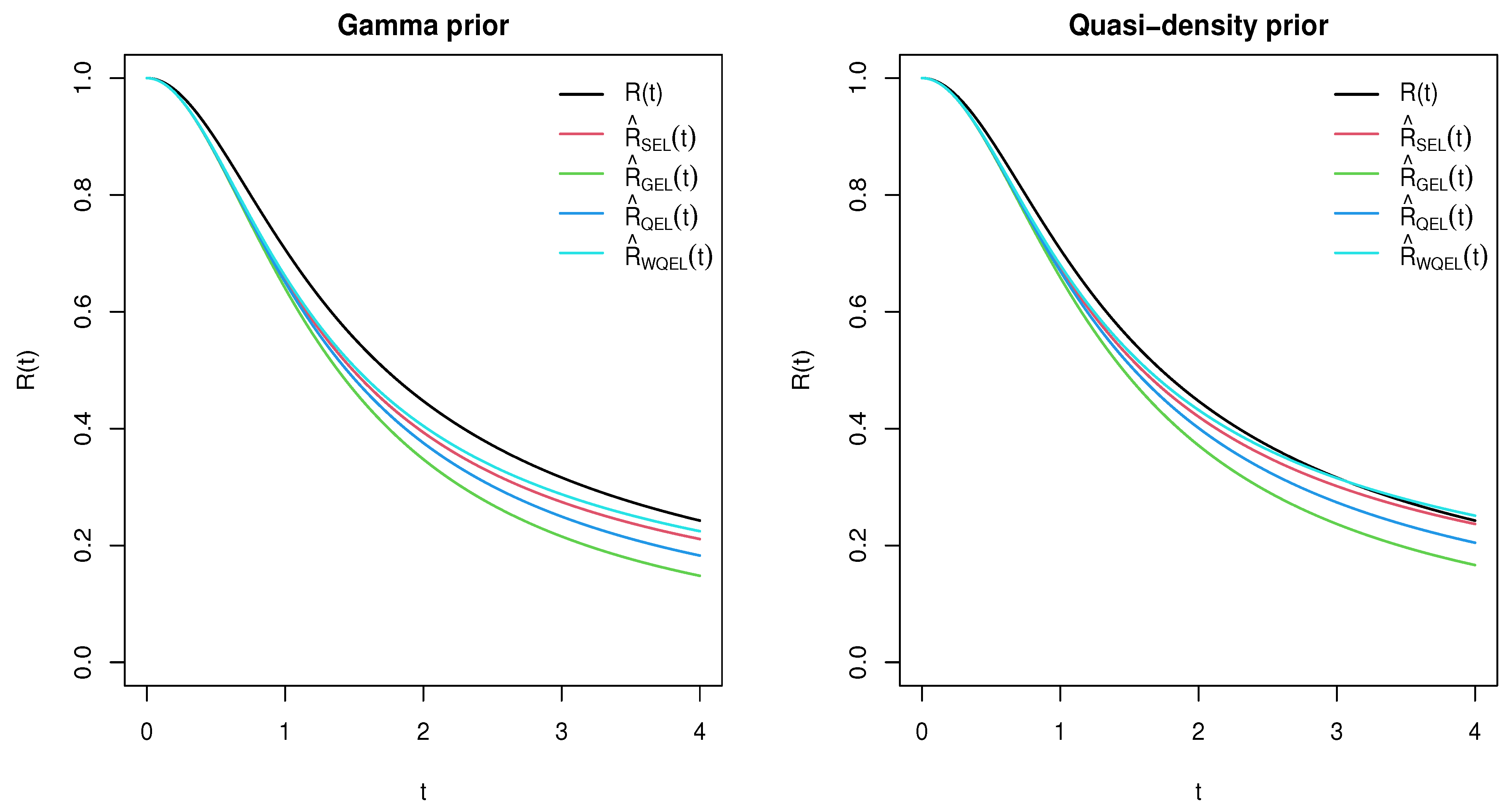
In order to provide an intuitive overview of the estimated reliability function under different estimators, Figure 5 and Figure 6 illustrate the differences between the Bayesian and classical estimators of the Burr XII distribution with the parameters and , assuming a sample size of . In Figure 5, the Gamma prior is set as , while the parameter in the quasi-density prior is set to . Meanwhile, the estimates under the SEL, GEL, QEL, and WQEL functions are compared for and .
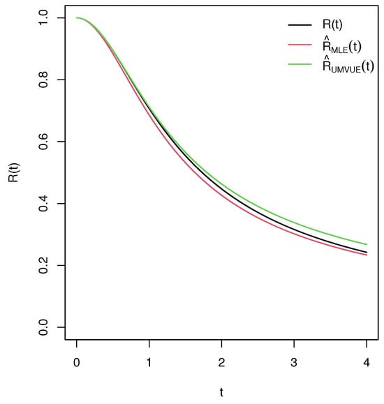
Figure 6.
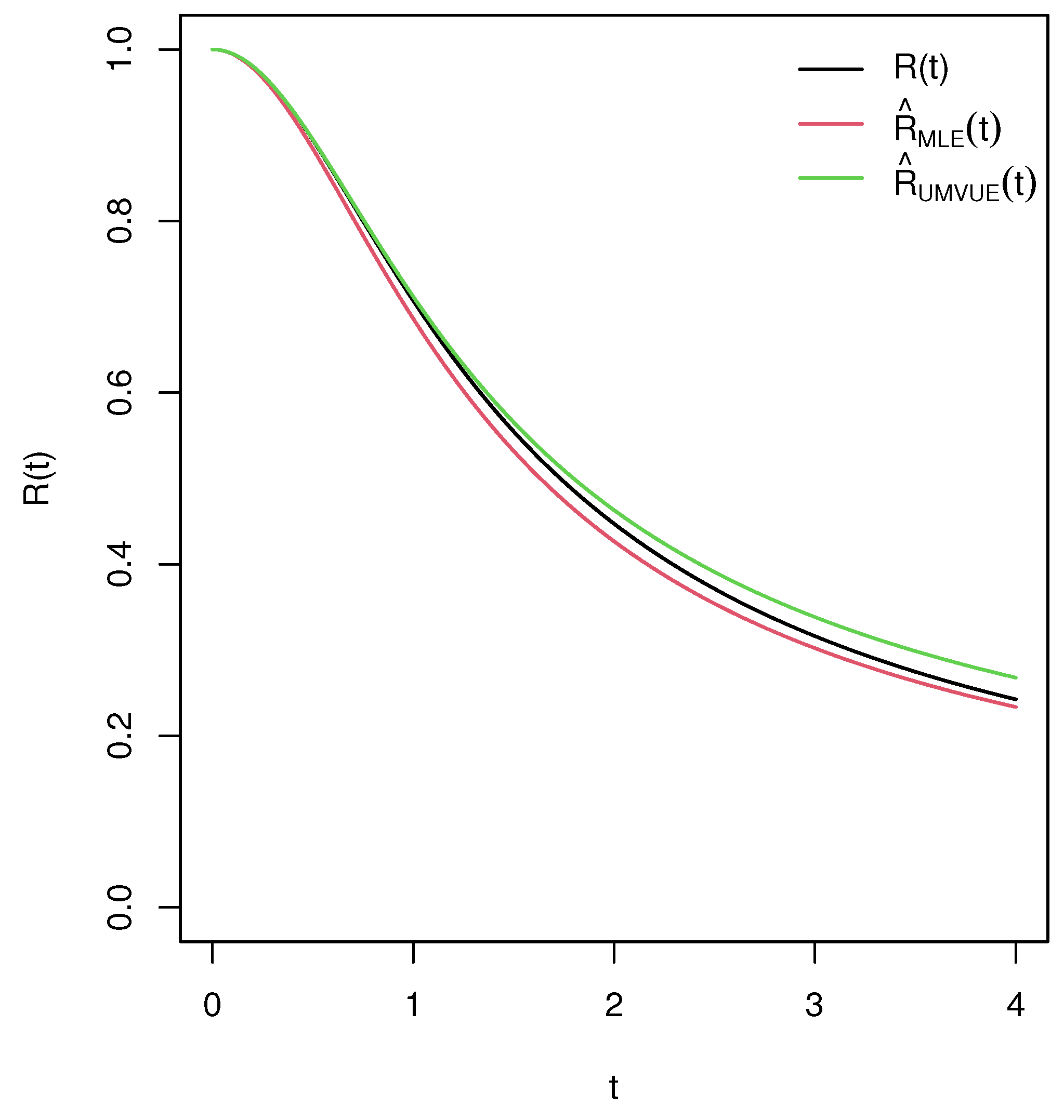
The MLE and UMVUE of the Burr XII distribution reliability function.
In Figure 5, it can be observed that the reliability functions estimated using the WQEL function are closer to the real value of , which indicates the superiority of the estimators under the WQEL function when compared with other estimators.
Figure 6 shows that as t increases, the estimated progressively approaches the true value of , whereas the UMVUE of progressively deviates.
6. Real Data Analysis
A real data set was employed in this section to illustrate the utility of the Burr XII distribution and its corresponding estimators. The data set comprises 128 observations recording the remission time (in years) of bladder cancer patients, as studied in [23]. An effective and accurate estimator of the reliability functions can greatly assist doctors in understanding the remission time of bladder patients globally and in managing the therapeutic interventions for these patients.
Before estimating the reliability of this data set, we initially calculated the Bayesian information criterion (BIC) for this data set for various commonly used lifetime distributions, including the Burr XII, Gamma, Weibull, Lindley, log-logistic, and linear–exponential distributions, to determine whether it is plausible to fit this data set with the Burr XII distribution.
The PDFs of the considered candidate distributions are structured as follows:
The goodness-of-fit results are shown in Table 6.
Table 6.
MLEs of the candidate models and their BICs on the data set.
The results in Table 6 show that the Burr XII distribution should be selected over the other candidate distributions due to its smaller BIC values.
In order to enhance the persuasive power of this study, a Kolmogorov–Smirnov test was conducted as a validation supplement. Let , , and denote the underlying distribution of the data, the estimated Burr XII distribution, and the empirical distribution, respectively. The test statistic for the null hypothesis versus the alternative hypothesis is shown below:
The Kolmogorov–Smirnov distance between the estimated Burr XII distribution and the empirical distribution was calculated as . This suggests that under a significance level of , there are no significant discrepancies between the estimated Burr XII distribution and the empirical distribution of the data. Moreover, the p-value of the test was calculated as . A high p-value indicates a high probability of obtaining the observed results, thus we cannot reject the null hypothesis, which verifies the correctness of choosing the Burr XII distribution as the best-fitting distribution.
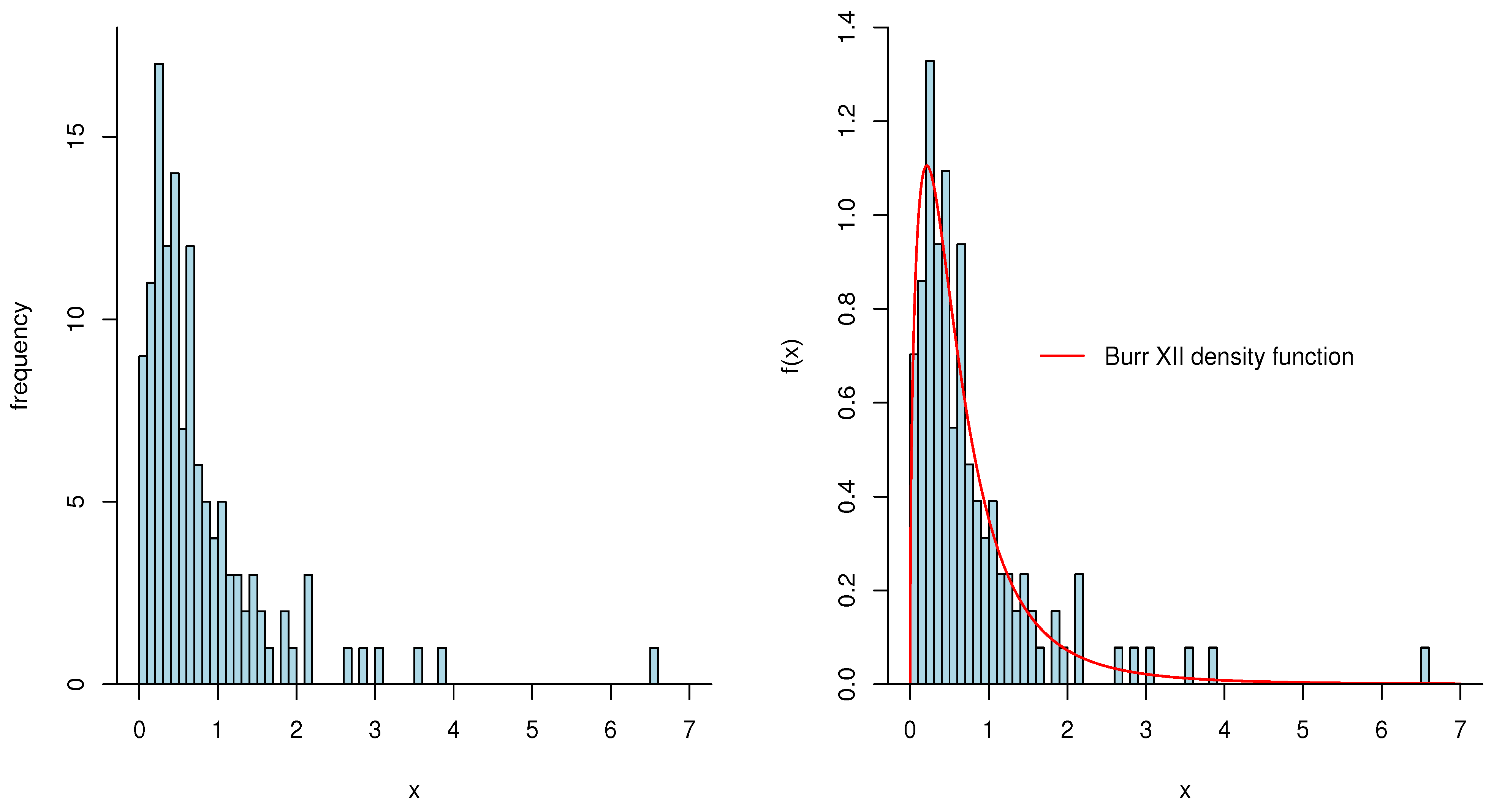
In order to visualize this data set more intuitively and compare it with the fitted Burr XII distribution, the histogram of the remission time data and the corresponding Burr XII distribution are shown in Figure 7. This suggests that both the histogram of the real data and the PDF of the underlying distribution exhibit similar patterns.
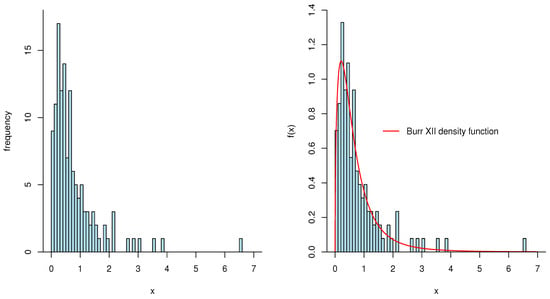
Figure 7.
Histogram of the remission time and its fitted Burr XII distribution.
Table 6 indicates that for the Burr XII distribution, the MLE of is . In order to verify that the real data are consistent with the case of a fixed and unknown as studied in this paper, we carried out a likelihood ratio test for the integrity of our studies using the Burr XII distribution. Let the null and alternative hypotheses be and , respectively. The test statistic is
Considering that approximately obeys a chi-square distribution with 1 degree of freedom, the p-value was calculated as , which indicates that under a significance level of , we cannot reject the null hypothesis. Therefore, we determined that the real data set obeys the Burr XII distribution with and unknown.
Consequently, the classical and Bayesian estimates for selected points of the reliability function of the remission time data are presented in Table 7. For the Bayesian estimates, we adopted the non-informative quasi-density prior with , and the parameters in the GEL, QEL, and WQEL functions were considered as , and , respectively.
Table 7.
The estimates of the reliability for selected points of the data set along with the corresponding running times.
In Table 7, it is evident that the running time of the estimator under the WQEL function was slightly longer than that of the other estimators, but the difference was not significant. Considering that the accuracy of the estimator under the WQEL function was better than that of the other estimators, such a time cost is acceptable.
7. Conclusions
Originating from the QEL function, we have proposed a new loss function called the WQEL and discuss the corresponding parameter and reliability function estimators of the Burr XII distribution under it. Classical estimators, including the maximum-likelihood and uniformly minimum-variance unbiased estimations, were also derived comprehensively. Considering Gamma and quasi-density priors, we discussed the estimators under the SEL, GEL, and QEL functions for Bayesian procedures and compared them with the estimators under the new loss function. Through Monte Carlo simulation, the estimator under the WQEL function was found to be superior to the other estimators, as can be seen in the tables and plots depicting the discussed estimators of the reliability function. Then, a remission time data set was analyzed to verify the applicability of the estimators introduced in this study. Before handling the data set with different estimators, we carried out BIC, Kolmogorov–Smirnov testing, and histogram procedures to confirm that the distribution underlying the real data was a Burr XII distribution. Finally, we presented the estimators of the reliability for the adopted data set.
We investigated frequentist and Bayesian inferences of the reliability function under the Burr XII distribution with a single unknown parameter and complete samples in this study. In future research, we expect to explore the corresponding estimators of the Burr XII distribution with double unknown parameters, as well as various censored schemes. We will also investigate the performance and provide specific guidance regarding the parameters of the new loss function in more cases and models.
Author Contributions
Investigation, K.H.; Supervision, W.G. All authors have read and agreed to the published version of the manuscript.
Funding
This research was supported by Project 202410004192 which was supported by National Training Program of Innovation and Entrepreneurship for Undergraduates.
Institutional Review Board Statement
Not applicable.
Informed Consent Statement
Not applicable.
Data Availability Statement
The data presented in this study are openly available in [23].
Conflicts of Interest
The authors declare no conflict of interest.
References
- Singh, U.; Gupta, P.K.; Upadhyay, S. Estimation of three-parameter exponentiated-Weibull distribution under type-II censoring. J. Stat. Plan. Inference 2005, 134, 350–372. [Google Scholar] [CrossRef]
- Krishna, H.; Kumar, K. Reliability estimation in Lindley distribution with progressively type II right censored sample. Math. Comput. Simul. 2011, 82, 281–294. [Google Scholar] [CrossRef]
- Han, M. E-Bayesian estimation of the reliability derived from Binomial distribution. Appl. Math. Model. 2011, 35, 2419–2424. [Google Scholar] [CrossRef]
- Nie, K.; Sinha, B.K.; Hedayat, A. Unbiased estimation of reliability function from a mixture of two exponential distributions based on a single observation. Stat. Probab. Lett. 2017, 127, 7–13. [Google Scholar] [CrossRef]
- Hamad, A.M.; Salman, B.B. On estimation of the stress-strength reliability on POLO distribution function. Ain Shams Eng. J. 2021, 12, 4037–4044. [Google Scholar] [CrossRef]
- Jha, M.K.; Dey, S.; Alotaibi, R.; Alomani, G.; Tripathi, Y.M. Multicomponent Stress-Strength Reliability estimation based on Unit Generalized Exponential Distribution. Ain Shams Eng. J. 2022, 13, 101627. [Google Scholar] [CrossRef]
- Liang, Q.; Yang, C.; Hu, S.; Huang, H. Reliability evaluation method of torpedo loading based on zero-failure data. Ocean. Eng. 2023, 278, 114431. [Google Scholar] [CrossRef]
- Alrumayh, A.; Weera, W.; Khogeer, H.A.; Almetwally, E.M. Optimal analysis of adaptive type-II progressive censored for new unit-lindley model. J. King Saud Univ. Sci. 2023, 35, 102462. [Google Scholar] [CrossRef]
- Ali, S.; Aslam, M.; Kazmi, S.M.A. A study of the effect of the loss function on Bayes Estimate, posterior risk and hazard function for Lindley distribution. Appl. Math. Model. 2013, 37, 6068–6078. [Google Scholar] [CrossRef]
- Han, M. A note on the posterior risk of the entropy loss function. Appl. Math. Model. 2023, 117, 705–713. [Google Scholar] [CrossRef]
- Khan, F.; Wang, H.; Yang, M. Application of loss functions in process economic risk assessment. Chem. Eng. Res. Des. 2016, 111, 371–386. [Google Scholar] [CrossRef]
- Razavi, M.; Sadoghi Yazdi, H.; Taherinia, A.H. Crowd analysis using Bayesian Risk Kernel Density Estimation. Eng. Appl. Artif. Intell. 2019, 82, 282–293. [Google Scholar] [CrossRef]
- Alduais, F.S.; Yassen, M.F.; Almazah, M.M.; Khan, Z. Estimation of the Kumaraswamy distribution parameters using the E-Bayesian method. Alex. Eng. J. 2022, 61, 11099–11110. [Google Scholar] [CrossRef]
- Al-Duais, F.S. Bayesian reliability analysis based on the Weibull model under weighted General Entropy loss function. Alex. Eng. J. 2022, 61, 247–255. [Google Scholar] [CrossRef]
- Alomari, H.M. A Comparison of Four Methods of Estimating the Scale Parameter for the Exponential Distribution. J. Appl. Math. Phys. 2023, 11, 2838–2847. [Google Scholar] [CrossRef]
- Polosin, V.G.; Mitroshin, A.N.; Gerashchenko, S.I. Burr Type XII Distribution in Traffic Control Systems. Transp. Res. Procedia 2023, 68, 433–440. [Google Scholar] [CrossRef]
- Jaheen, Z.F.; Okasha, H.M. E-Bayesian estimation for the Burr type XII model based on type-2 censoring. Appl. Math. Model. 2011, 35, 4730–4737. [Google Scholar] [CrossRef]
- Rastogi, M.K.; Tripathi, Y.M. Estimating the parameters of a Burr distribution under progressive type II censoring. Stat. Methodol. 2012, 9, 381–391. [Google Scholar] [CrossRef]
- Tahir, M.; Abid, M.; Aslam, M.; Ali, S. Bayesian estimation of the mixture of Burr Type-XII distributions using doubly censored data. J. King Saud Univ. Sci. 2019, 31, 1137–1150. [Google Scholar] [CrossRef]
- Yan, W.; Li, P.; Yu, Y. Statistical inference for the reliability of Burr-XII distribution under improved adaptive Type-II progressive censoring. Appl. Math. Model. 2021, 95, 38–52. [Google Scholar] [CrossRef]
- Seyed Rasuol Hosseini, E.D.; Jamkhaneh, E.B. The Bayesian and Bayesian shrinkage estimators under square error and Al-Bayyati loss functions with right censoring scheme. Commun. Stat. Simul. Comput. 2022. [Google Scholar] [CrossRef]
- Ozkan, O.; Kilic, S. A Monte Carlo Simulation for Reliability Estimation of Logistics and Supply Chain Networks. IFAC-PapersOnLine 2019, 52, 2080–2085. [Google Scholar] [CrossRef]
- Lemonte, A.J.; Cordeiro, G.M. An extended Lomax distribution. Statistics 2013, 47, 800–816. [Google Scholar] [CrossRef]
Disclaimer/Publisher’s Note: The statements, opinions and data contained in all publications are solely those of the individual author(s) and contributor(s) and not of MDPI and/or the editor(s). MDPI and/or the editor(s) disclaim responsibility for any injury to people or property resulting from any ideas, methods, instructions or products referred to in the content. |
© 2024 by the authors. Licensee MDPI, Basel, Switzerland. This article is an open access article distributed under the terms and conditions of the Creative Commons Attribution (CC BY) license (https://creativecommons.org/licenses/by/4.0/).