Abstract
Mainstream transferable adversarial attacks tend to introduce noticeable artifacts into the generated adversarial examples, which will impair the invisibility of adversarial perturbation and make these attacks less practical in real-world scenarios. To deal with this problem, in this paper, we propose a novel black-box adversarial attack method that can significantly improve the invisibility of adversarial examples. We analyze the sensitivity of a deep neural network in the frequency domain and take into account the characteristics of the human visual system in order to quantify the contribution of each frequency component in adversarial perturbation. Then, we collect a set of candidate frequency components that are insensitive to the human visual system by applying K-means clustering and we propose a joint loss function during the generation of adversarial examples, limiting the frequency distribution of perturbations during attacks. The experimental results show that the proposed method significantly outperforms existing transferable black-box adversarial attack methods in terms of invisibility, which verifies the superiority, applicability and potential of this work.
1. Introduction
With the increasing application of deep neural networks (DNNs), adversarial examples have also received increasing attention due to their threat to the security of DNNs. The latest research on adversarial attacks has focused on more realistic black-box attack scenarios [1,2], where attackers are assumed to have no knowledge of the target model. In particular, the transferability of adversarial examples has received significant attention recently. Many existing works such as [1,2,3,4] focus on generating transferable adversarial examples by leveraging substitute models, which has significant implications for DNN deployment since transferable adversarial examples can attack various models that are irrelevant with substitute models. However, in black-box scenarios [5,6], noticeable artifacts in adversarial examples may raise the suspicions of the model owner and thus render the attack method impractical. Therefore, guaranteeing the invisibility of adversarial perturbation is critical for black-box adversarial attacks.
Currently, the norm is the most common metric for measuring and constraining the visual difference between adversarial examples and clean ones, which, however, does not fit the human visual system (HVS) well [7]. Recent research [8] has also demonstrated that the constraint is insufficient to guarantee the invisibility of adversarial examples; i.e., adversarial examples may introduce noticeable distortion although the norm between adversarial examples and clean ones can be small [9,10]. To deal with this problem, we draw inspiration from HVSs, which show that different frequency information in images allows for different perturbation strengths while remaining invisible to HVSs. Hence, we propose analyzing adversarial attacks from the frequency domain.
We analyzed the robustness of a DNN model in the Fourier domain. Our results indicated that the generalization and robustness of a model should be jointly determined by the training dataset and the network structure of the model. It can be said that DNN models are commonly more sensitive to certain frequencies in the Fourier domain. In contrast to previous works [11,12], we found that perturbations in both low and high frequencies can result in good attack effects. This insight inspires us to design adversarial perturbations from the perspective of the Fourier domain. By analyzing the frequency sensitivity of DNNs and the HVS characteristics of input samples, we quantify how perturbations in different frequency components affect the transferability and invisibility of adversarial examples. By adjusting the frequency distribution used for generating adversarial perturbation, the invisibility of transferable adversarial attacks can be significantly enhanced.
In summary, the main contributions of this work include the following:
- We propose an invisible adversarial attack method based on Fourier analysis, where the derivation and superposition of adversarial perturbations are performed in the frequency domain, thus avoiding the drawbacks to adversarial attacks due to the use of norm constraints.
- We propose a new optimization objective for adversarial attacks in the Fourier domain, using a joint adversarial loss and frequency loss for optimization. Unlike previous works that mainly focus on generating adversarial examples in the spatial domain and use the norm to constrain the strength of perturbation, which is insufficient for the invisibility of adversarial examples, our analysis of the Fourier domain characteristics of adversarial examples offers a new perspective for further research.
- We have conducted extensive experiments to evaluate the proposed method and compare it with existing transferable adversarial attack methods. The results show that the proposed method significantly enhances the invisibility of adversarial attacks.
2. Related Works
2.1. Black-Box Adversarial Attacks
Black-box adversarial attacks assume that the attacker only knows the output of the target model such as the final prediction and confidence score. Black-box attacks typically include two categories, i.e., query-based attacks and transfer-based attacks. In this paper, we focus on the latter attack and thereby assume that the attacker can only utilize a surrogate model to generate adversarial perturbations without the right to query the target model, which is more suitable for application scenarios.
Fast gradient signed method (FGSM)-based attacks [1,2,3,4,10,13,14], which rely on the transferability of adversarial examples, are the most effective among various black-box attacks. For example, Kurakin et al. [10] enhance the transferability of adversarial examples by introducing the basic iterative method (BIM), also known as the iterative FGSM (I-FGSM). However, the adversarial examples generated by the I-FGSM are prone to overfitting to local optima, which can affect the transferability of the adversarial examples. To deal with this problem, Dong et al. [3] introduce the momentum iterative FGSM (MI-FGSM), which incorporates the concept of momentum into the I-FGSM. The MI-FGSM stabilizes the gradient update direction, effectively passes through local optima, and further enhances the transferability of adversarial examples.
In addition to optimization techniques, model augmentation is also a powerful strategy. For example, Xie et al. [4] solve the overfitting problem of the I-FGSM by using image transformation techniques and named it the diverse iterative FGSM (DI-FGSM). To alleviate the problem of excessive reliance on substitute models, Dong et al. [2] shift the input, create a series of images, and approximately solve the total gradient. Lin et al. [14] use the scale invariance property of DNNs to average the image gradients of different scales to update adversarial examples.
Although these methods have good transferability, they often generate adversarial examples with obvious traces of modification. To address this problem, Ding et al. [15] made improvements to the iterative process of I-FGSM-like algorithms by proposing a selective I-FGSM, which ignores unimportant pixels in the iterative process according to first-order partial derivatives, thus compressing the perturbations and significantly reducing the adversarial example’s image distortion. Wang et al. [16] are concerned about the neglect of global perturbation for image content/spatial structure, which can result in leaving obvious artifacts in otherwise clean regions of the original image, and therefore propose to adaptively assign perturbations based on the Just Noticeable Difference (JND) of the human eye by adaptively adjusting the perturbation strength by using the pixel-by-pixel perceptual redundancy of the adversarial example as a loss function. Similarly, Zhang et al. [17] add the JND of the image as a priori information to the adversarial attack and project the perturbation into the JND space of the original image. Furthermore, they add a visual coefficient to adjust the projection direction of the perturbation to consciously equalize the transferability and invisibility of the adversarial example. Such content-specific adaptive perturbation is inspiring, and they all analyze the effect of image content on the invisibility of perturbation in terms of the spatial domain, whereas the characteristics of the image such as the structure, texture, and so on, are dependent on the distribution of the frequency information. Thus, the approaches of analyzing invisible adversarial attacks in terms of the Fourier domain enable a more comprehensive understanding of the characteristics of the adversarial attack, and we will explore them from the perspective of image frequency information.
2.2. Frequency Principle of Adversarial Examples
Currently, research on the principles of adversarial examples suggests that shallow feature maps of neural networks typically extract edge and texture features, which highlights the importance of high-frequency information for final classification. In [18], Luo et al. theoretically prove the frequency principle (FP) for DNNs through analyzing the spectral response and spectral deviation of DNNs. They reveal the causes and effects of the FP, demonstrating that DNNs exhibit a significant bias towards the information of different frequencies during decision making. The dependence of the model on high-frequency signals is also directly related to the phenomenon of adversarial examples. Zhang et al. [12] propose a practical attack method without a box that introduces small but effective perturbations through a hybrid image transformation (HIT) without changing the semantic information of the image. The authors demonstrate that the HIT can effectively deceive multiple target models and detectors with low computational costs and high success rates.
However, recent research indicates that the conclusion that adversarial examples are high-frequency perturbations is incorrect. In detail, Maiya et al. [19] propose a frequency-analysis-based method for quantifying the adversarial robustness of DNNs. The authors first define a novel frequency sensitivity index (FSI) to measure the model’s sensitivity to perturbations in different frequency ranges. The analysis shows that adversarial examples do not rely only on high or low frequencies, but the impact of the used dataset should be considered.
3. Methodology
3.1. Preliminaries
3.1.1. Adversarial Attack
Let represent a DNN that maps the raw domain to the target domain . In this paper, we limit the DNN to image classification, indicating that corresponds to a number of images, and is a set of classes. Given a sample , an attacker aims to construct a perturbation that the perturbed sample, also called adversarial example, successfully deceives , i.e., . Specifically, in the untargeted attack scenario, this causes the model’s classification to deviate from the original label, and in the targeted attack scenario, this causes the model to classify the samples to the target label.
White-box adversarial attacks produce adversarial examples directly on the target model, which does not work for black-box attacks. To realize successful black-box attacks, a common strategy utilizes a substitute model to generate adversarial examples, which are then used to attack the black-box models, leveraging transferability. Black-box models with various structures are used to simulate the possible target models.
For compactness, let denote the substitute model and denote B black-box models that are independent of . The structures of these models can be different from each other. In the targeted attack scenario, the goal of the attack is to construct adversarial examples with such that these adversarial examples are misclassified as a specified incorrect class by , . For the untargeted attack scenario, the output is not limited to a particular incorrect class.
Mathematically, given a sample , generating the adversarial example with can be formulated as the following problem:
subjected to , where is the loss function and is a threshold given in advance. Existing adversarial attack methods often use cross-entropy loss. The strength of perturbation is constrained by the norm to control the visual differences between the adversarial examples and clean ones. Existing adversarial attacks typically use [20], [9,21], and [9,10,21] to control the perturbation in the spatial domain.
3.1.2. Frequency Domain Robustness
By evaluating the response of DNNs to different frequencies of noise, we can analyze the frequency domain robustness of DNNs [22]. In detail, given an image, every element in the Fourier matrix contains information about the corresponding frequency component and appears as a plane wave in the spatial domain. After shifting the zero-frequency component to the center of the matrix, the distance of each element from the center point describes the frequency of the plane wave. The direction towards the center point represents the direction of the plane wave, and the value of the element represents the amplitude of the plane wave. We put the perturbation in the frequency information of the plane wave, leaving all Fourier matrices’ imaginary parts unchanged. We generate a unit perturbation on each frequency component separately, which gives us Fourier basis noises. We apply Fourier basis noises to the three-color channels with coefficients randomly selected from the set and perturb RGB images using different frequencies separately. After applying Fourier basis noises, we can establish a function between the classification error rate of the model on the noisy test set and the frequency domain information of the noise, which can be visualized as the Fourier heatmap of the model.
3.2. Motivation
In the current field of AI research, researchers are committed to improving the performance of AI systems and many approaches have been proposed including upgrading the model structure, training algorithms, and improving the quality of deployed data, among others, from the field of data-centric and model-centric AI [23]. Adversarial attack research is significant in both fields. Research on adversarial attacks can make adversarial examples more challenging, which is crucial for data-centric AI research to help us better understand the impact of training data on model robustness. In addition, advances in the field of adversarial attacks can lead us to design more robust model structures and guide strategies and techniques for model defense, thereby improving model security and reliability.
In addition to the importance in AI research, high-quality adversarial examples play an important role in many other real-world scenarios of applications, especially in terms of privacy protection, e.g., securing the privacy of social network users. In big data environments such as social media, where people’s personal information and private data can be subject to various forms of attacks and violations, the use of adversarial samples can help protect users’ private data from unauthorized exploitation. Users upload and share adversarial examples of their photos instead of clean photos, which makes it more difficult for the model to identify and utilize personal information and does not affect the photo sharing experience, thus effectively increasing the level of privacy protection for users on social media platforms. Such scenarios place higher demands on the transferability and invisibility of adversarial examples.
Existing works based on the I-FGSM and model augmentation are effective in improving the transferability of adversarial examples while leaving obvious traces of modification. Additionally, recent research [8] demonstrates that constraints in the pixel domain are insufficient to guarantee the visual quality of adversarial examples. Due to the limitations of the I-FGSM, attackers can only use the constraint of the norm to implicitly ensure that the visual distance between adversarial examples and clean ones is not too large, which is insufficient for invisibility.
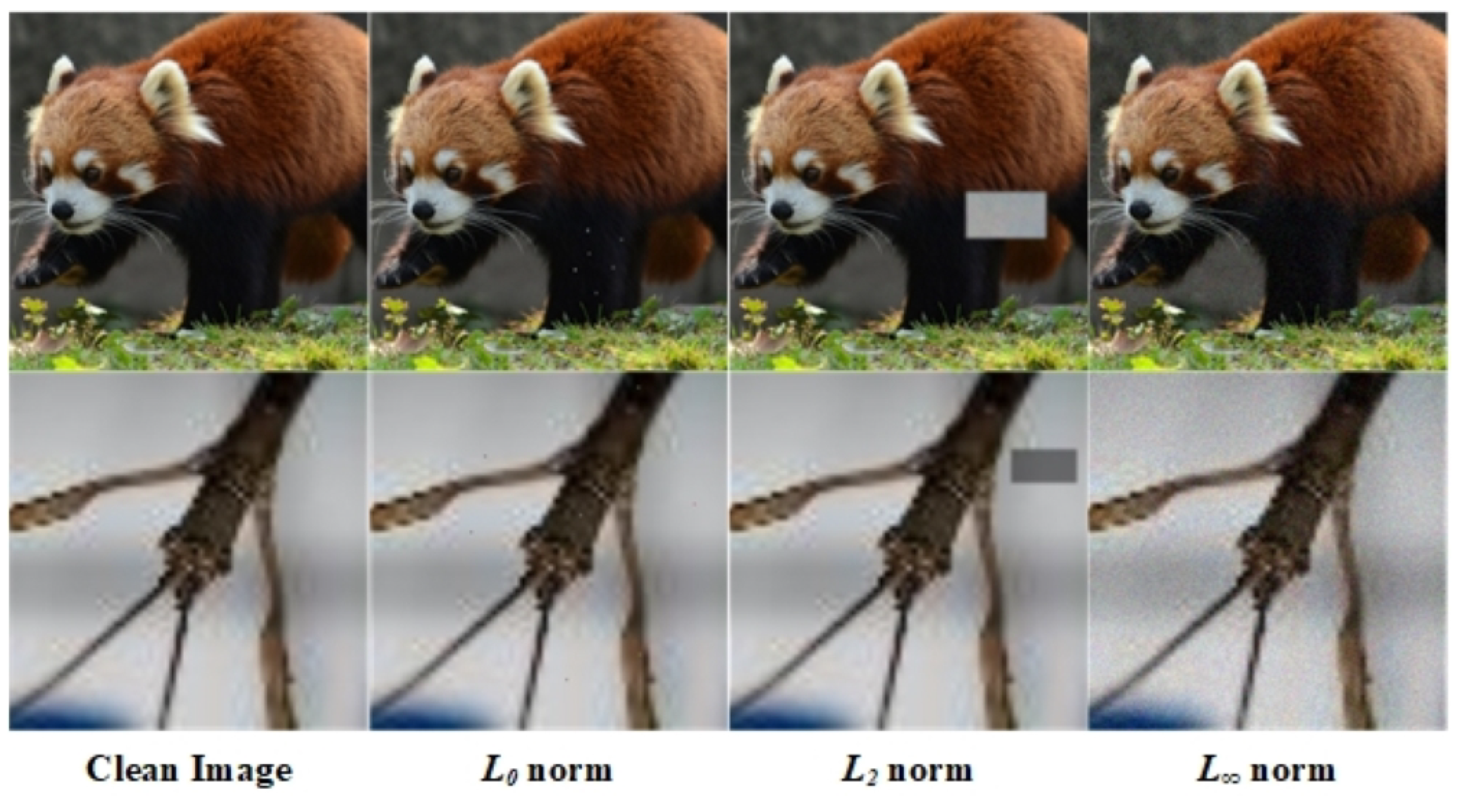
The norm measures the number of different pixels between two images, the norm measures the Euclidean distance between two images, and the norm measures the maximum difference between corresponding pixels in two images. These norms only constrain certain statistical characteristics of perturbations in the pixel domain and may not ensure the invisibility of adversarial examples. Figure 1 displays an attack instance that uses only the norm to constrain the perturbation strength, revealing the significant limitations of constraints.

Figure 1.
Perturbed images with small , , and norm constraints can still exhibit distinct perceptual artifacts; the two examples are from Tiny-ImageNet [24]. Specifically, a single pixel’s perturbation value can be extremely large with a small norm. An uneven perturbation may deceive the norm constraint, but it is visually apparent. The norm constrains the maximum perturbation amplitude on every single pixel in the images. Still, a uniform perturbation may have a small maximum value but a large average strength, which can seriously affect the visual perceptual quality of images.
The use of norms can be misleading; that is, adversarial examples with small norms are visually similar to clean images, but this is not the case. Nearly all adversarial attacks directly modify image pixels in the spatial domain based on the gradient information of the model, making it difficult for perturbations to adapt to changes in image content and often leaving visible traces.
The perception of visual signal changes varies for different visual content. The human visual system (HVS) [7] is a non-uniform and nonlinear image processing system that acts as a low-pass linear system in the frequency domain. Due to its limited resolution, the HVS is more sensitive to changes in low-frequency image signals compared to high-frequency ones. While DNNs perceive image information counterintuitively, differently to the HVS, image information that is unrecognizable to the human eye may be important to DNNs, and they can use high-frequency information that is not visible to the human eye to achieve correct judgments. Perturbations to such information can be less visible to the human eye, while being able to significantly influence the decision of the DNNs. The attempt to incorporate biological principles into the design of algorithms [25,26], such as the “Attention Mechanism”, provides a new way of thinking; i.e., the properties of HVSs can be used in the analysis of adversarial attacks. Hence, we analyze the process of adversarial attacks from a frequency domain perspective and explore the relationship between the invisibility, transferability, and frequency domain distribution of perturbations.
3.3. Fourier Domain Analysis
The study of adversarial examples from the frequency perspective [18,19,22] suggests a close correlation between the occurrence of adversarial examples and a DNN’s preferences for different frequency information during the classification process. To further explore the frequency domain characteristics of adversarial examples, we first analyze the frequency domain robustness of DNNs by building Fourier heatmaps.
In a Fourier heatmap, the heat value of each element of the Fourier matrix represents the average test error of the model under the noise of the corresponding frequency component. Our Fourier heatmaps revealed that DNNs have distinct sensitivity to input information of different frequencies, and there is a specific sensitivity for each frequency component. We tested the frequency domain sensitivity of DNNs with different network structures on some commonly used classification datasets, and found that this correspondence between the frequency domain sensitivity of DNNs and frequency domain components is universal.
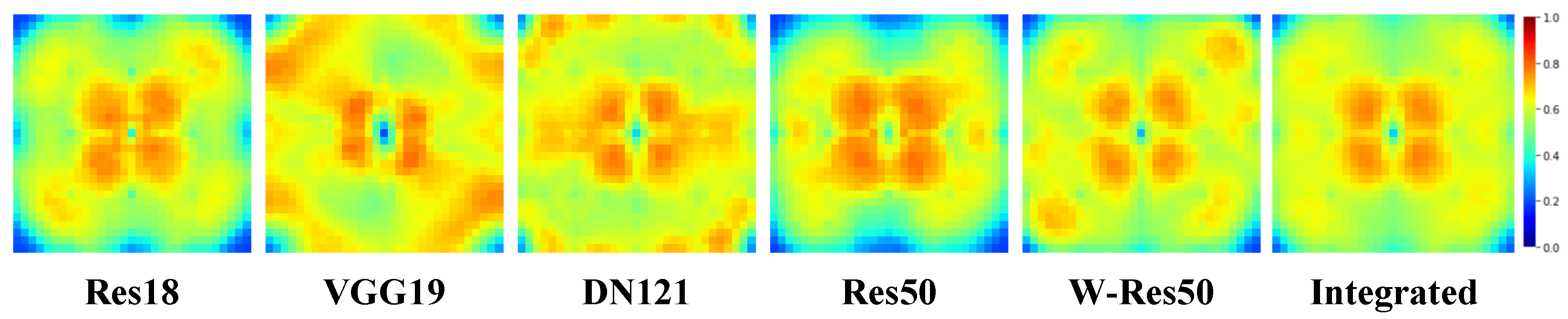
We trained multiple DNN models with different structures on the commonly used image classification datasets CIFAR10 [27], CIFAR100 [27], and Tiny-ImageNet [24]. Taking the CIFAR10 dataset as an example, we present in Figure 2 the Fourier heatmaps of different DNNs. The red regions in the figure correspond to the areas with the largest test error, indicating that the model is most sensitive to changes in these frequency domain components.
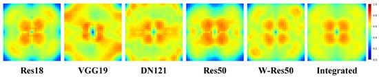
Figure 2.
Fourier heatmaps of various DNN models tested on the CIFAR10 dataset, where we used Res50 [28], Res18 [28], VGG19 [29], DN121 [30], and W-Res50 [31]. The heat value of each pixel represents the average test error of the corresponding DNN model under the noise of a particular frequency component. The heat value is confined to the range and represented by a color scale. As the legend indicates, larger heat values correspond to redder colors, while smaller ones correspond to bluer colors.
It is evident that the sensitive regions of different models overlap. We extracted the points with the highest test error from the heatmap to identify these regions, selecting an extraction region of of the entire matrix. We assigned “1” to these regions and “0” to others and obtained a binary mask. They represent the weakest Fourier regions of frequency domain robustness to the noise of DNNs on this dataset.
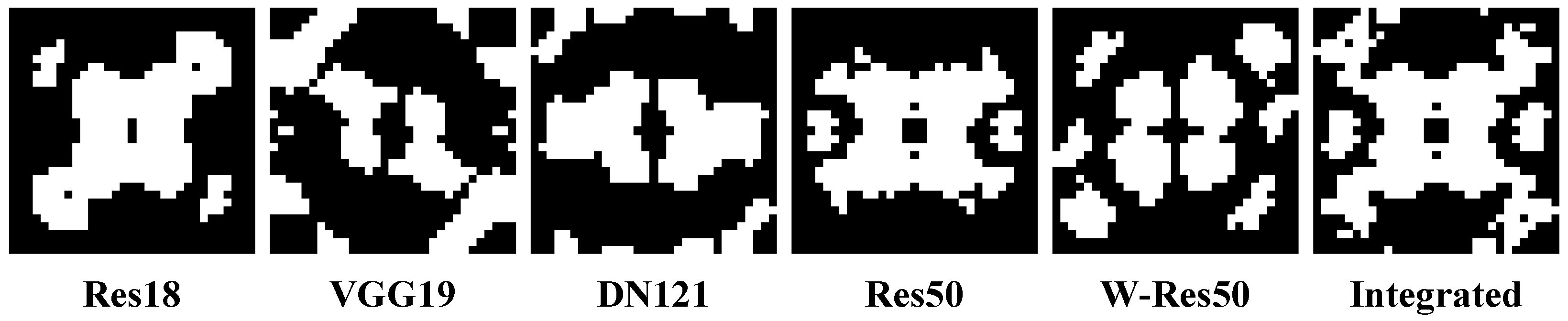
Figure 3 shows the binary masks of different models. Regions with “1” denote sensitive regions, and regions with “0” denote non-sensitive regions. It is evident that different DNNs have significant overlap in their sensitive regions, indicating that their frequency domain robustness is quite similar. Combined with previous studies on the robustness of neural networks [22], we argue that the frequency domain robustness of a DNN is jointly determined by the statistical characteristics of the training dataset and the structure of its network. Therefore, integrating the sensitive regions of DNNs with diverse structures can reduce interference from the network structure and random factors during the training process, leading to a more precise common sensitive region of DNNs. We integrated the masks of multiple models on the same dataset and obtained an integrated binary mask by removing isolated points that appear in only one mask. Placing adversarial perturbations from the Fourier domain over these common regions is naturally expected to generate a stronger attack effect on the DNN models.
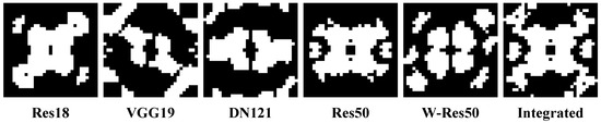
Figure 3.
Frequency domain sensitive region masks for different DNN models on the CIFAR10 dataset. By adding up the masks of all models, we set the values of points with a value of 1 in two or more masks to 1 and set the value of points with a value of 1 in only one mask or a value of 0 in all masks to 0, resulting in an integrated mask .
All DNNs on the same dataset exhibit weaker robustness to perturbations of specific frequency domain components; this insight motivates us to explore adversarial attacks from a frequency domain perspective.
The HVS is affected by many factors, forming some visual laws that can be utilized. The HVS can be understood as a frequency decomposition system, which can decompose the spatial information of the input image into different frequency components, and has different sensitivities to different components of spatial frequency. The contrast sensitivity function (CSF) is an index that is specifically used to evaluate the response of the HVS to visual stimuli of different frequencies. Based on a large number of experiments, Mannos and Sakrison [32] proposed the CSF model based on a large number of experiments using mathematical tools such as the Fourier transform to characterize the relationship between HVS sensitivity and spatial frequency, which was later improved by Daly [33] as:
where is the spatial frequency and and are the spatial frequencies in the horizontal and vertical directions, respectively. According to this model, for medium- and high-frequency information of an image, the sensitivity of the human eye is approximately inversely proportional to the frequency; i.e., the invisibility of a perturbation should be positively correlated with the height of its frequency, and the sensitivity of the visual perception decreases markedly in the high-frequency region. By constraining perturbations to components with higher frequencies, we can increase the invisibility of adversarial examples while maintaining their transferability.
As we group the adversarial attack process from the Fourier frequency domain, the modification of the perturbation to each pixel value of the image is converted into a modification of the information at each frequency, and therefore the gradient information should also reflect how the change in the information at each frequency in the input to the model affects the model’s output and loss function. First, we transform the input image to the frequency domain using the Fourier transform and denote it as :
We turn it back on the spatial domain and put it into the DNN to compute the loss function. Back-propagation calculates the gradient information of the loss function for the output of the model and utilizes the chain rule and the differentiability of the neural network to complete the gradient calculation and propagation from the output layer to the input layer. Since both the Fourier transform and the Fourier inverse transform are differentiable, based on the chain rule, we can add them to the process of back-propagation by converting the gradient of the loss function with respect to the input to the gradient with respect to its frequency domain information and obtain the partial derivatives of the loss function with respect to . During the back-propagation process, the gradient information can be formulated as follows:
where represents the Fourier transform and represents the inverse Fourier transform. Then, the gradient information is used to update and finally obtain an adversarial example after the inverse Fourier transform.
3.4. Attack Algorithm
Based on the above Fourier domain analysis for adversarial attacks, we propose an invisible transferable adversarial attack in this subsection.
Several studies from a model-based perspective have argued that the decision boundary and the model architecture of a substitute model all have a significant impact on adversarial transferability [34]. Since the possible target model is completely unknown, the use of model augmentation to reduce the dependence on the decision boundary of the substitute model is a common strategy for transferable adversarial attacks [1,2,4]. Here, we use frequency domain model augmentation [1] and combine it with the Fourier sensitivity analysis of DNNs to make the augmentation more directed. Specifically, we transform the model input to the Fourier domain and apply noise addition and enhancement to redirect the perturbation toward the common frequency-sensitive regions of DNNs. The augmentation can be formulated as follows:
where ⊙ represents the Hadamard product, the multiplicative noise is uniform noise sampled from a uniform distribution, that is, , and the additive noise is set to Gaussian noise .
Specifically, we add frequency domain noise to the model input in the Fourier domain, improving the transferability of adversarial examples. Next, we quantitatively analyze the impact of different frequency components of perturbations on the transferability and invisibility of adversarial examples. We employ a clustering analysis to select the most valuable regions in the Fourier domain for adversarial attacks, which guide the adjustment direction of the frequency domain distribution of the perturbation. We propose a frequency domain loss, using it alongside adversarial loss, and we use the cross-entropy loss here as the joint loss function to derive and design the perturbation from the Fourier domain.
We propose to combine the frequency domain robustness of DNNs and the frequency characteristics of the HVS to perform the adversarial attack from the frequency domain and enhance the invisibility of the transferable adversarial examples. The details are given in Algorithm 1. As shown in Algorithm 1, our method can be divided into three stages. Firstly, we transfer the input image to the frequency domain and perform frequency domain augmentation. Then, we take back-propagation of the joint loss function in the Fourier domain and update the adversarial example by applying a frequency domain step size of while ensuring that the pixel values are in the normal range by normalization.
| Algorithm 1 Fourier invisible adversarial attack. |
|
It is worth noting that the noise processing for the input image may make the direction of the gradient information unstable, so we perform N times random initializations of the frequency domain augmentation noise and perform propagation N times, obtaining the gradient information . By averaging , the average gradient can stabilize the update direction of the counter perturbation. We will explain the design of each step in the algorithm in detail in the following sections.
3.5. Cluster Analysis
The previous analysis has demonstrated that DNNs possess shared sensitive characteristics for specific frequency domain components in the Fourier domain regarding adversarial examples. Noise in these frequency domain components is more likely to deceive the neural network. Moreover, as we discussed earlier, the frequency of perturbations is closely linked to their invisibility. In the Fourier domain, the visual perceptual sensitivity of the HVS to perturbations is likewise closely related to its frequency and decreases significantly for high-frequency perturbations. Hence, we analyze the optimization objectives of perturbations in the Fourier domain, integrating both frequency sensitivity and invisibility.
Observing the frequency-domain-sensitive regions of the DNN, as shown in Figure 3, it can be found that a substantial part of the common frequency-domain-sensitive regions of the neural network exist in low-to-medium frequency regions. Therefore, when constraining the perturbation to the frequency-sensitive region, we need to consider the effect of the frequency of the perturbation on the visibility.
For the process of adversarial attacks, each element in the Fourier matrix embodies two characteristics of the perturbation of a frequency component. On the one hand, the heat value in the Fourier heatmap reflects the sensitivity of the DNN to perturbations in this frequency domain component. The higher the heat value , the greater the probability of the perturbation causing the target model to classify incorrectly. On the other hand, based on the CSF model, it can be concluded that for the middle- and high-frequency bands in which the common sensitive region of the DNN are located, the CSF and the spatial frequency can be approximated as being inversely related. Correspondingly, the CSF reflects the human eye’s ability to perceive details at different frequencies, so for the same intensity of perturbation, the higher its frequency, the weaker the human eye’s ability to perceive the details and therefore the better its invisibility; i.e., the invisibility of the perturbation is positively correlated with its frequency. Consequently, we use the distance from the pixel point to the zero-frequency component (after frequency centering) to represent the invisibility of the perturbation at that frequency. These two characteristics of perturbation correspond to the requirements of transferability and invisibility of adversarial examples, which we define as:
Through the function of the frequency domain component of perturbation, the heat value , and the frequency , we can transform the improvement in the invisibility of transferable adversarial examples into the filtering of each element in the Fourier matrix in a two-dimensional space composed of the heat value and frequency . Placing perturbations in the area with the highest heat value can improve the transferability of adversarial examples, while placing all perturbations in the area with the highest can minimize the visual difference between adversarial examples and original images.
A clustering algorithm [35] is the process of clustering similar samples together based on the distribution law of the sample data themselves. We use a clustering algorithm to filter common sensitive regions in the Fourier domain and obtain the optimal embedding regions conducive to the invisibility of adversarial examples. We take all elements in the sensitive regions as a set, denoted as C, and use the K-means algorithm [35] to cluster them. The K-means algorithm is based on calculating the distance between samples and center points to induce the target function of each cluster under its own samples, which is:
Here, we normalize the values of and and set the weight of the two through the coefficient to adjust the bias towards the transferability and invisibility of adversarial examples. We first initialize K cluster centers in the clustering process, where K is set to 2. Then, each sample is classified by calculating its distance to the cluster center, and the position of the cluster center is recalculated until all samples are classified.
Through the clustering algorithm, we divided the common sensitive regions of the DNN in the Fourier domain into two parts: the low-frequency region with a low heat value and a low value for the adversarial attack, and the high-frequency region with a high heat value and high value for the adversarial attack. It should be noted that and do not simply represent high and low frequencies but rather relatively high or low frequencies after weighing the heat value and frequency.
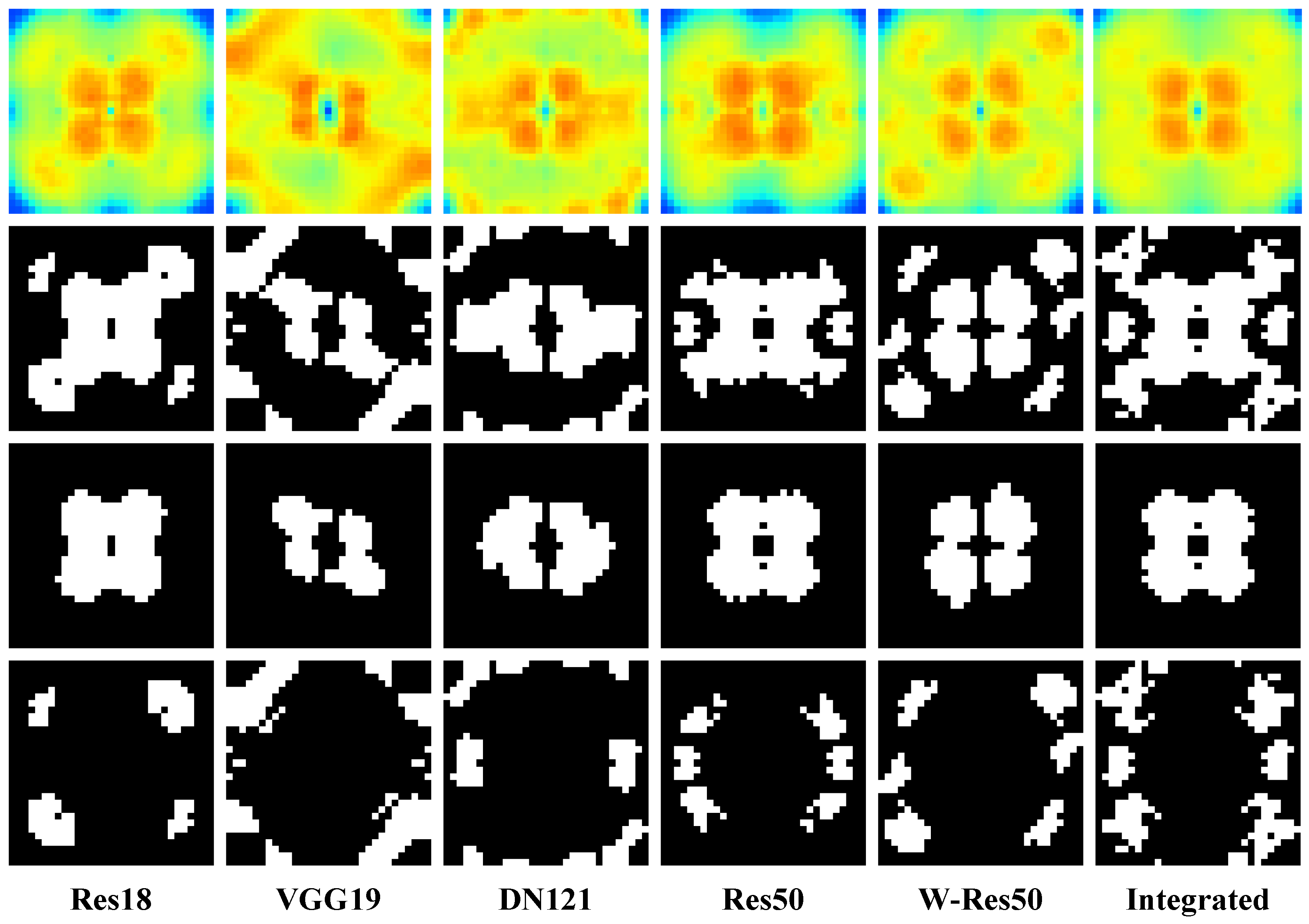
Figure 4 shows the clustering results of the sensitive regions on the CIFAR10 dataset. Comparing the results of the different models and integrated result, it is obvious that the distributions of low-frequency regions and high-frequency regions of the DNNs do have obvious common characteristics, which again confirms our proposed view that the frequency domain robustnesses of DNNs are common.
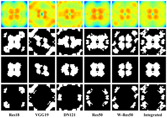
Figure 4.
Results after the clustering mask on the CIFAR10 dataset, with the Fourier heatmap, sensitive regions, low-frequency regions, and high-frequency regions from top to bottom by row.
Through a quantitative analysis, we divide the common sensitive region and use the result as the optimization target in the Fourier domain for the adversarial attack. We will discuss further how to redirect the frequency domain distribution of the perturbation toward this region by frequency domain constraints in the next section.
3.6. Frequency Domain Loss
Typically, many adversarial attacks directly use the adversarial loss function as the optimization objective while simply constraining the perturbation through the Lp norm, which is obviously insufficient for an attack method that has requirements for image quality. Some studies add image evaluation functions such as SSIM [6], JND [16] constraints, etc., to the optimization objective as penalty terms to solve it, but this simple restriction on the strength of the perturbation may lead to an unsuccessful attack on the DNN.
We propose that in addition to the strength of a perturbation, its frequency domain distribution can also affect the performance of the adversarial example. Therefore, we propose a new optimization objective that adds the frequency domain loss to adjust the perturbation. Specifically, we divide the loss function of the adversarial attack into the adversarial loss and frequency domain loss, and we formulate the frequency domain optimization as the maximization process of the frequency domain loss. We find the region with the highest value in the Fourier domain for the adversarial attack; then, we can improve the efficiency of the adversarial attack by optimizing the perturbation frequency domain distribution.
Through a clustering analysis, we divided the overall Fourier matrix into a low-frequency region , a high-frequency region , and a non-sensitive region , where E is the all-ones matrix; we name them the frequency mask set . Then, all the information of the perturbation on the frequency domain can be formulated as:
where , and represent the perturbation strength of the disturbance in the low-frequency region, high-frequency region, and non-sensitive region, respectively:
For the overall perturbation, the value of is the lowest for the adversarial attack, so we constrain it; furthermore, within the sensitive region, we further optimize the perturbation based on the HVS, which has greater visual redundancy for and lower redundancy for , so we concentrate the perturbation on . We can summarize the frequency optimization objectives of the adversarial attack as increasing and constraining and , formulated as:
To adjust the frequency domain distribution of the perturbation, the easiest way is to use the strength of the perturbation in each frequency domain region directly as the frequency domain loss. However, this method may lead to the problem of overfitting; if the strength of perturbation in a certain frequency domain is too large, it will obscure the antagonistic loss during back-propagation and the strength of the perturbation will vary greatly during the iterative process so that simple superposition will lead to unstable gradients.
Therefore, we use the ratio of the strengths of the perturbation in different regions as the loss function, so we set frequency domain loss as:
In the optimization process, the strength of the perturbation may be zero, so we add a tiny factor to the denominator to avoid a zero denominator. We use and as the numerator and as the denominator to form the frequency domain loss, respectively. Moreover, we set the frequency domain loss to a negative value to avoid increasing the gradient.
The use of the frequency domain loss can adjust the frequency domain distribution of the perturbation by minimizing the fractional equation and increasing in exchange for decreasing and . Since the DNN has a high sensitivity to the perturbation within , by reducing the unnecessary frequency domain components in the non-sensitive region, we can achieve an adversarial attack with a lower perturbation strength. In addition, placing the perturbation more in the high-frequency region can improve the overall invisibility of the adversarial examples.
4. Experimental Results and Analysis
4.1. Experiment Setup
4.1.1. Datasets
We selected the three most commonly used image classification datasets: CIFAR10 [27], CIFAR100 [27], and Tiny-ImageNet [24]. They contain 10, 100, and 200 labels with image shapes of , , and , respectively; 13,000, 18,000, and 28,000 images from the training set are chosen as the validation set to build the Fourier heatmap of the DNN.
4.1.2. Backbone Network
All the models we used achieved good results in the image classification task. In the experimental part, we consider representative DNNs as black-box models , namely Resnet50 [28], Resnet18 [28], VGG19 [29], DenseNet-121 [30], and Wide-Resnet50 [31] (denoted as Res50, Res18, VGG19, DN121, and W-Res50, respectively). All experiments in this paper were conducted in the PyTorch environment using a single RTX Titan GPU.
We trained all models on the above three datasets and used SGD as an optimizer. The learning rate was set to and was dynamically adjusted using a scheduler with momentum set to . The number of epochs was 100, and the batch size was 64.
Our proposed method is general and independent of the DNN structure and can be applied similarly to any existing pre-trained classifier. In the experiments, to avoid errors due to a single model structure and to ensure the reliability of experiment results, we employed multiple substitute models and comprehensively evaluated their performance against attacks by exchanging between substitute models and black-box models.
4.1.3. Comparative Methods
We choose the baseline I-FGSM [10] and PGD method [9] and various state-of-the-art attack methods, DI-FGSM [4], -FGSM [1], MI-DI-FGSM [4], and TI-DI-FGSM [2], as comparative methods to evaluate our proposed attack methods from multiple perspectives such as invisibility, transferability, etc.
Among them, the MI-DI-FGSM and TI-DI-FGSM are the combination of two adversarial attacks. The MI-DI-FGSM was proposed by Xie et al. [4], and adds diverse inputs (DIs) to momentum iteration (MI-FGSM) [3]; the TI-DI-FGSM was proposed by Dong et al. [2], and adds a translation invariant attack (TI) to the DI-FGSM.
4.1.4. Parameter Settings
For all experiments, we set the parameters of all algorithms as follows: maximum perturbation constraint , number of iterations , step size , and noise initialization times .
For our proposed algorithm, we constructed neural network models for constructing Fourier heatmaps on each dataset which are independent of the black-box models . We integrated the results of different networks and set the extraction percentage of sensitive regions to and the weighting factor to in K-means clustering, obtaining sensitive regions and high-frequency regions , as shown in Figure 5. For the frequency domain augmentation, we set the multiplicative noise to and the standard deviation to for Gauss noise, and we set the frequency step size to on CIFAR100 and tiny-ImageNet, and to 15 on CIFAR10. To fairly evaluate the effectiveness of the proposed method, as with comparative methods, we added constraints on the perturbations in the null domain, limiting the perturbations to the same strength for all methods, i.e., .
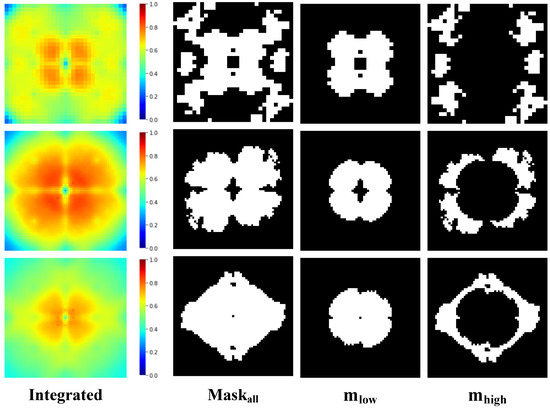
Figure 5.
The division of Fourier domain regions by K-means clustering on the three datasets. After the clustering mask on the CIFAR10, CIFAR100, and Tiny-ImageNet datasets, the results are shown from top to bottom by row. The integrated Fourier heatmap sensitive regions and the low-frequency and high-frequency regions after clustering are shown from left to right by column.
For the parameter setting of the comparative methods, we set the transformation probability to for the DI-FGSM. For the MI-DI-FGSM, we set the transformation probability to and the decay factor of the momentum iteration to . For the TI-DI-FGSM, the transformation probability was also , and the kernel length of the translational transformation was 7. For the -FGSM, we set the tuning factor to and the standard deviation of Gaussian noise set to .
4.1.5. Attack Scenarios
In the experimental part, we randomly selected clean images from the test set of each dataset for the adversarial attack and used all models to correctly classify these images. To ensure fairness, we used the same images for different attack methods in the same scenario.
For the untargeted attack scenario, we generated 2000 adversarial examples for each attack method using a selection of 2000 clean images for each dataset. In the targeted attack scenario, we randomly selected 200 images from each dataset and conducted targeted attacks on all labels except the original ones. In CIFAR100 and Tiny-ImageNet, the classification confidence of the substitute model’s target labels served as a filter; we retained the attack results for the top 10 target labels with the highest confidence for each clean image, resulting in 2000 adversarial examples per attack method for evaluating the optimal performance of the targeted attack. The CIFAR10 dataset contains only nine additional labels besides the original label, so we included all the attack results on these labels. This resulted in 1800 adversarial examples, which were used to assess the average performance of the attack methods in the targeted attack scenario.
4.1.6. Evaluation Matrix
For the evaluation of transferability and invisibility, we used the same substitute model for different attacking methods to generate adversarial examples in the same attack scenario and tested them using the same black-box models.
We evaluated the transferability of adversarial examples on the black-box models. In the targeted attack scenario, the black-box model should classify the adversarial examples to the target labels outside the original labels for a successful transfer attack. In the untargeted attack scenario, the adversarial examples are considered to have a successful transfer attack as long as the black-box model misclassifies them. The transfer success rates of the adversarial examples on the black-box models evaluate the transferability of the attacking methods.
In terms of evaluating the image quality of adversarial examples, the norm ensures that the perturbation strength set by all methods is consistent. We employed multiple metrics to evaluate examples from various perspectives; all used evaluation metrics are as follows: Peak Signal-to-Noise Ratio (PSNR) [36], Structural Similarity Index (SSIM) [36], Root Mean Squared Error (RMSE), Universal Quality Image Index (UQI) [37], Erreur Relative Globale Adimensionnelle de Synthèse (ERGAS) [38], Visual Information Fidelity (VIF) [39], and Learned Perceptual Image Patch Similarity (LPIPS) [40].
4.2. Evaluation of Image Quality
4.2.1. Tiny-ImageNet
The image quality of adversarial examples was evaluated under both untargeted and targeted attack scenarios, and the average values of the metrics for all the adversarial examples of different methods are presented in Table 1, where the up arrow indicates that for this metric, a higher value is better, while the down arrow indicates the opposite. Under the premise of the same perturbation strength constraints of all attack methods, our method outperforms others on various image evaluation metrics.

Table 1.
Performance of different attacking methods in terms of image quality on Tiny-ImageNet. The best results are presented in bold.
The data in Table 1 show that in the target attack scenario, compared with the DI-FGSM algorithm, which performs relatively well in comparison to other methods, the average PSNR of our adversarial examples is higher by about 4–6 dB. There is a significant improvement in all the evaluation metrics of image quality and invisibility, such as VIF and LPIPS. The data for the untargeted attack reflect similar results to those for the targeted attack. Compared with the other methods, our examples show significant improvement in all image evaluation metrics on all substitute models, with an average PSNR improvement of about 4–8 dB. This indicates that our adversarial attack also applies to the untargeted attack scenario and performs well on the invisibility of the adversarial examples in both attack scenarios.
In addition, through cross-model comparison of the adversarial examples on different substitute models, it can be found that although there are some differences in the image quality of adversarial attacks on each model due to variations in network structures, the relative performance of all attacking methods is consistent. This indicates that adversarial attacks do not depend on a specific network structure, and our method can be applied to various substitute models.
4.2.2. CIFAR100 and CIFAR10
Similarly, we conducted experiments on the CIFAR10 and CIFAR100 datasets to evaluate the image quality of adversarial examples. We used the same backbone network Res50 as the substitute model in Tiny-ImageNet and evaluated both untargeted and targeted attack scenarios. We report the average values of all evaluation metrics of the generated adversarial examples in Table 2.
Table 2.
Performance of different attacking methods in terms of image quality on CIFAR100 and CIFAR10.The best results are presented in bold.
The above experimental data show that under different attack scenarios and different experimental settings on alternative models, the generated adversarial examples of our method on multiple datasets outperform the comparison methods in terms of image quality and invisibility. This also confirms the correctness of our frequency domain analysis for adversarial attacks; i.e., by constraining the adversarial perturbation’s frequency domain distribution, we can effectively improve the invisibility of the generated adversarial example, which we will continue to prove in later experiments.
4.3. Visualization Analysis
In former experiments, we demonstrate our improvement to comparative attacking methods regarding invisibility, and we will evaluate the impact of adversarial attacks by visualizing the image details of adversarial examples.
4.3.1. Detail Comparison
We visually compare the image details of the adversarial examples generated by attacking methods. In the same experimental setup as before, we compare examples generated in the same alternative model under the same attack scenario.
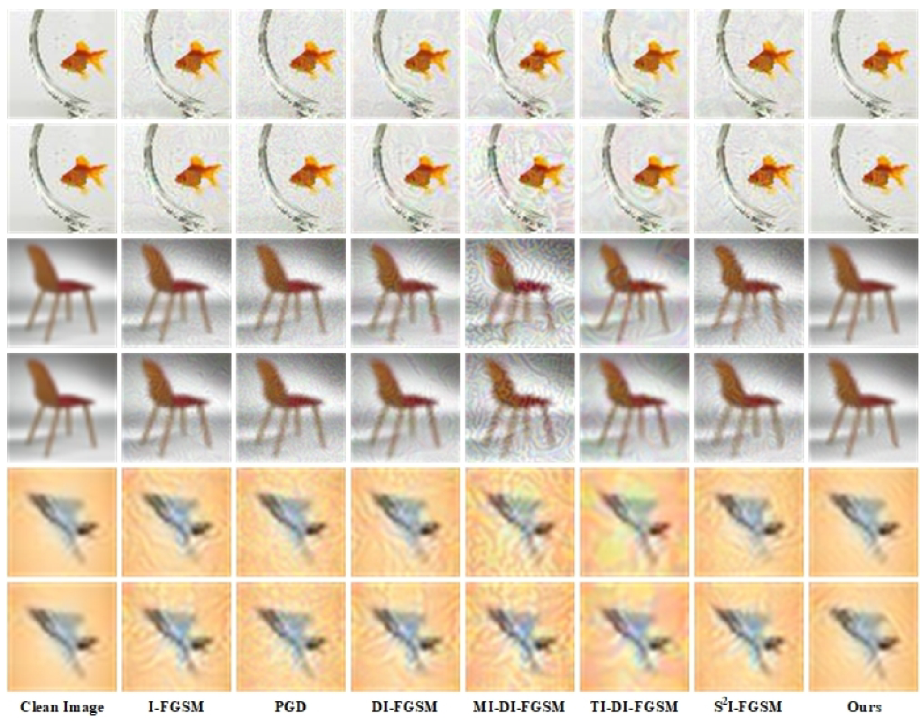
In Figure 6, we show the adversarial examples generated by all methods on the substitute model Res50. The adversarial perturbation generated by the comparison method has a very obvious impact on the visual quality of the examples and leaves visual traces in the smooth region of the image. In contrast, the adversarial examples generated by our method have little impact on the smooth region of the image and have a significantly better visual quality than those of the other methods, which are closer to the original image for the HVS. The results in the targeted attack and untargeted attack scenarios reflect the same phenomenon: the perturbation generated by the comparison method significantly affects the visual quality of the examples on all three different datasets. In comparison, our perturbation significantly reduces the impact of relatively smooth regions in the images.
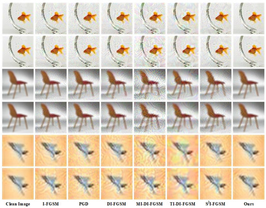
Figure 6.
Comparison of the image details of the adversarial examples of the attacking methods. These adversarial examples come from the Tiny-ImageNet, CIFAR100, and CIFAR10 datasets from top to bottom by two rows. For each dataset, the upper row shows the targeted attack scenario, and the lower row shows the untargeted attack scenario. The leftmost column shows the original clean images. The adversarial examples generated by different methods are listed from left to right.
The comparative methods measure the overall change in pixel values of images using norms, which ignores image content and leads to visible traces in smooth regions. We design the perturbation from the frequency domain and restrict the frequency domain distribution of the perturbation to the high-frequency region, which has less effect on the visibility, significantly improving the invisibility of the adversarial examples.
4.3.2. Difference Analysis
To further analyze the impact of attacks on images, we visualize the adversarial perturbations using an absolute difference map.
Taking the adversarial examples in untargeted attack scenario on the Tiny-ImageNet dataset as an example, we differentiate the adversarial example from the original image, take the absolute values, and visualize the absolute difference maps on the three RGB channels. Due to the constraints of the norm, the maximum perturbation of all the adversarial examples is set to . We normalize all the absolute difference maps to 0∼255, where 0 and 255 represent black and white, respectively. The larger the perturbation value of that point, the brighter the pixel point.
In Figure 7, we show the absolute difference maps of perturbations in the three channels of the image for the comparative methods and our proposed method. The perturbations generated by the comparative methods in each channel exhibit meaningless noise patterns, with the perturbation strength in each region being approximately uniform, especially evident in the maps of PGD. In contrast, our absolute difference maps exhibit clear distribution patterns of perturbations in all three channels. Our perturbations are mainly concentrated in regions of the image with complex contents, but have little effect on the smooth regions of the image.
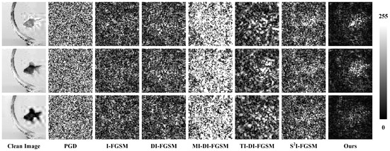
Figure 7.
Absolute difference maps of the adversarial examples and clean image, where each column from top to bottom is the perturbation of the three channels R, G, and B. All absolute difference maps are normalized from 0 to 255, where 0 and 255 are represented in black and white.
From the above analysis, it can be concluded that our method adapts the perturbations to the image content and significantly reduces the influence on the smooth regions of the image, i.e., the regions where the low-frequency component accounts for more. We transferred the perturbations to high-frequency regions where the human visual system is less sensitive, thus making the generated adversarial examples have minimal visual differences compared to the original images.
4.4. Evaluation of Transferability
To verify the transferability of our proposed attack methods, we tested all comparative attacking methods’ transfer success rates on black-box models. In the same way as in the experiments above, we tested on three datasets with the substitute model Res50 to test the performance of each method in targeted and untargeted attack scenarios.
Table 3 shows the transfer success rates of the black-box models in the targeted attack scenario using different attacking methods; the results of the experiments on Tiny-ImageNet, CIFAR100, and CIFAR10 are shown from top to bottom. Each row represents the transfer success rate on different black-box models.
Table 3.
Transfer success rate of attacking methods on three datasets (from top to bottom: Tiny-ImageNet, CIFAR100, and CIFAR10).
The experimental results in the table show that in the challenging targeted attack scenario, the adversarial examples generated by our method have good transferability, which indicates that our proposed adversarial attack method has a good performance on the invisibility of adversarial examples and good transferability.
In the untargeted attack scenario, the DNN’s classification of the adversarial sample only needs to deviate from the original label to determine the success of the adversarial attack, which significantly reduces the attack difficulty compared to the targeted attack scenario. Table 3 shows the transfer success rates of attacking methods in an untargeted attack scenario; the results of the experiments on Tiny-ImageNet, CIFAR100, and CIFAR10 are shown from top to bottom. The data in the table show that our method also has significantly higher transferability success rates compared to the TI-DI-FGSM, which is one of the most transferable adversarial attacks available, indicating that our method also outperforms others in an untargeted attack scenario.
4.5. Ablation Study
4.5.1. Quantitative Analysis in the Frequency Domain
To quantitatively analyze the perturbation of adversarial attacks on images and verify the effectiveness of our proposed method, we conducted a statistical analysis of the perturbations of a large number of adversarial examples from the perspective of the Fourier domain to examine the frequency domain characteristics of the perturbations generated by our method.
The strength and proportion of low-frequency perturbations can reflect the invisibility of the adversarial examples. By counting the proportion of low-frequency perturbations in the total perturbation strength of all generated adversarial examples, we can summarize the distribution pattern of perturbations of comparative methods.
In the previous discussion, we divided the Fourier matrix into three parts, and we used the masks as filters to calculate the perturbation strength in different frequency bands using the norm. The strength of the perturbations in these different frequency bands represents the amount of modification of the image’s corresponding frequency information. We count the average low-frequency perturbation strength on the region and the percentage of low-frequency perturbations in the total perturbation strength.
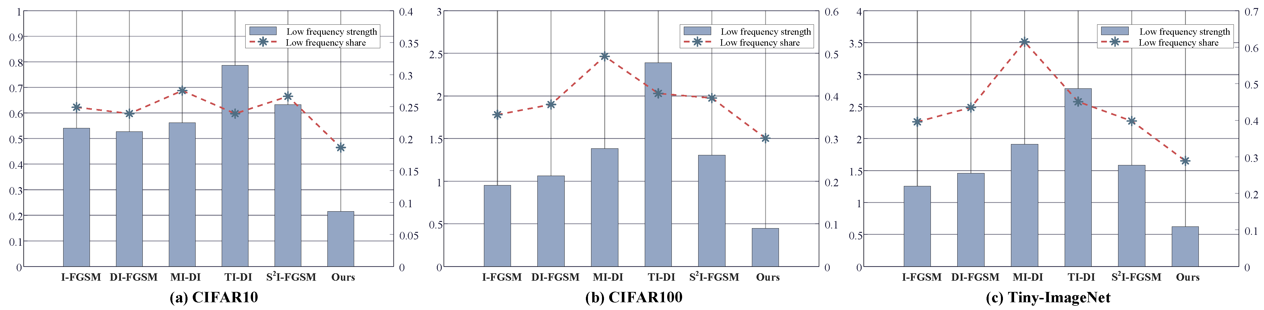
Figure 8 shows the frequency domain characteristics of comparative methods on the Tiny-ImageNet, CIFAR100, and CIFAR10 datasets, respectively. The histogram data in the figures represent the average strength of low-frequency perturbations of adversarial examples. The line plot data represent the proportion of low-frequency perturbations for different methods. The histogram data in the figure show that our method has the smallest average low-frequency perturbation strength. Moreover, the line plots reflect that the proportion of low-frequency perturbations in the adversarial perturbations of our method is also the lowest compared to comparative methods. This illustrates that the proposed optimization objective is effective, which successfully limits the perturbation to the HVS-insensitive high-frequency region while improving the performance of the adversarial examples.
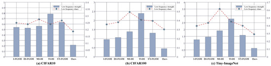
Figure 8.
Average low-frequency perturbation strength and low-frequency perturbation share of different methods on CIFAR10 (a), CIFAR100 (b), and Tiny-ImageNet (c). Here, the MI-DI-FGSM and TI-DI-FGSM are denoted as MI-DI and TI-DI, because of length.
4.5.2. Fourier Perturbation Hotspot Map
To further analyze the distribution pattern of perturbations of the adversarial attack in different frequency bands, we average the perturbations over all examples and visualize the frequency domain characteristics of the average perturbations.
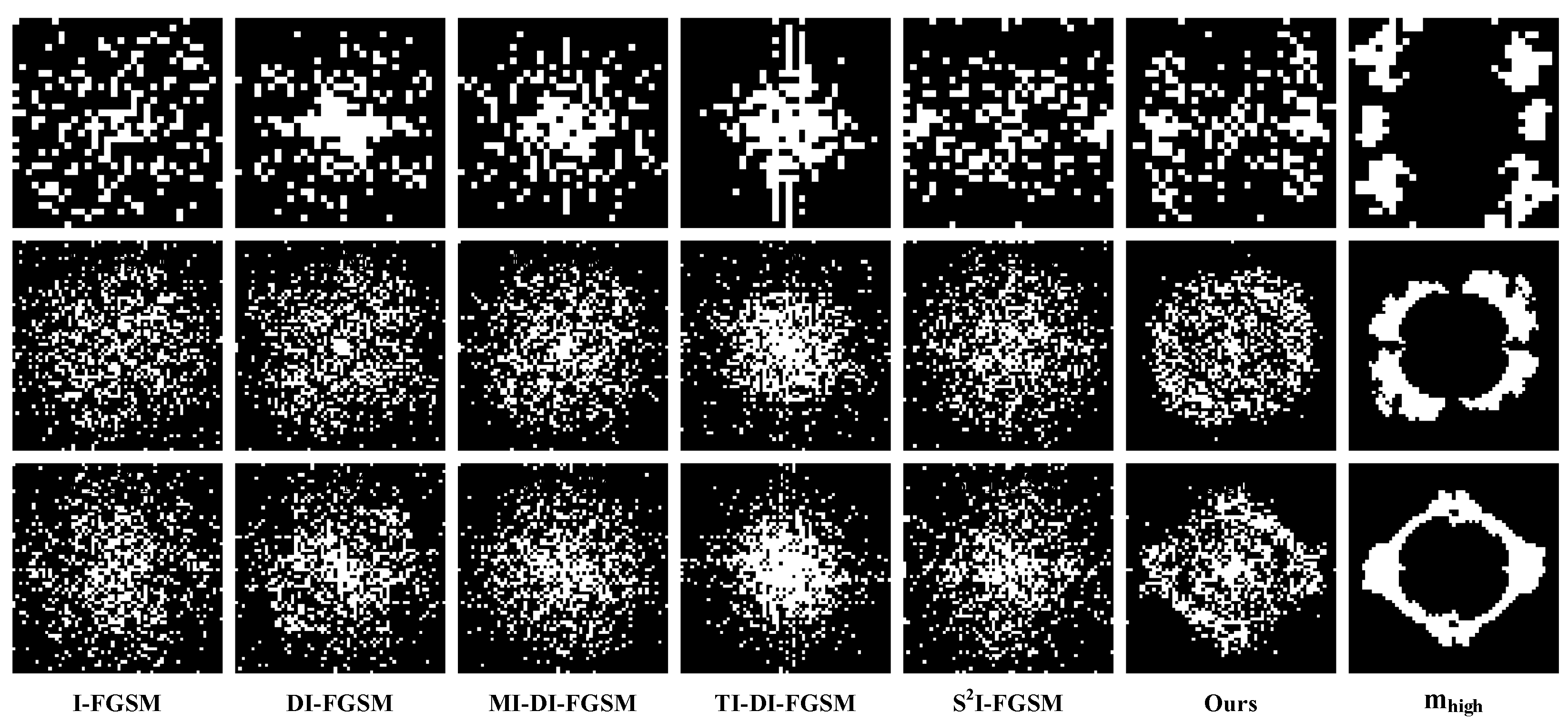
We use a similar processing method as the Fourier heatmap to Fourier transform the average perturbation and obtain a Fourier map with the values of its elements representing the strength of the perturbation in this frequency domain component. Then, we extract the strongest region with the maximum value of of the Fourier map and binarize it. We call the binarized map the Fourier perturbation hotspot map. The Fourier perturbation hotspot maps for all methods are shown in Figure 9. The proposed method successfully aligns the frequency domain distribution of the perturbations with high-frequency sensitive regions of the DNN. This further supports the conclusion that the proposed frequency loss function was effective and successful.
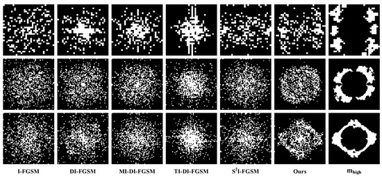
Figure 9.
Fourier perturbation hotspot plots of the comparative attacking method. From top to bottom are the experimental results on CIFAR10, CIFAR100, and Tiny-ImageNet datasets, where the rightmost column is the high-frequency region in Figure 5.
5. Conclusions and Discussion
In this work, we analyze the process of adversarial attacks from the perspective of the Fourier domain and propose an invisible adversarial attack, which significantly improves the invisibility of the transferable adversarial examples. We compute the gradient and superimpose the perturbation from the frequency domain and then quantify the impact of different Fourier frequency components of perturbations on the transferability and invisibility of adversarial examples, so as to establish a target region that can balance the transferability and invisibility through the K-means clustering algorithm. We propose to use the adversarial loss and the loss in the frequency domain as a joint optimization objective to constrain the frequency-domain distribution of the perturbation towards the target region. The experimental results show that the proposed designs are effective and the performance of the adversarial examples is significantly improved.
Most research on transferable adversarial attacks focuses on how to simulate black-box models through model augmentation to improve the success rate of transfer attacks. We hope to provide a new perspective beyond the conventional spatial domain perspective; we can also explore the intrinsic principles of adversarial examples through frequency analysis. This may help solve the problems of adversarial attacks that are currently difficult to solve in the spatial domain.
The common frequency-sensitive characteristics of DNNs are of great significance for future research on adversarial attacks; for example, more robust black-box DNN watermarking can be constructed based on these characteristics [41]. Further exploration may help to improve the performance of adversarial attacks, the interpretability of the attacks, and the understanding of the generalization ability of DNNs. Due to the limitation of the experimental equipment, this study uses a limited number of DNNs to construct the common frequency-sensitive region. By adding more structurally rich models, a more accurate common frequency-sensitive region of DNNs can be obtained, providing stronger support for further research in the field of adversarial attacks.
Author Contributions
Conceptualization, C.L., X.Z. and H.W.; Data curation, C.L. and Y.L.; Formal analysis, C.L. and Y.L.; Methodology, C.L. and X.Z.; Software, C.L. and Y.L.; Supervision, X.Z. and H.W.; Writing—original draft, C.L.; Writing—editing, H.W. All authors have read and agreed to the published version of the manuscript.
Funding
This research was funded by the National Natural Science Foundation of China (NSFC) under Grants U22B2047.
Institutional Review Board Statement
Not applicable.
Informed Consent Statement
No applicable.
Data Availability Statement
Publicly available datasets were analyzed in this study. The datasets can be found here: https://www.cs.toronto.edu/~kriz/cifar.html (accessed on 13 March 2024) and http://cs231n.stanford.edu/tiny-imagenet-200.zip (accessed on 13 March 2024).
Conflicts of Interest
The authors declare no conflicts of interest.
References
- Long, Y.; Zhang, Q.; Zeng, B.; Gao, L.; Liu, X.; Zhang, J.; Song, J. Frequency domain model augmentation for adversarial attack. In Proceedings of the European Conference on Computer Vision, Tel Aviv, Israel, 23–27 October 2022; pp. 549–566. [Google Scholar]
- Dong, Y.; Pang, T.; Su, H.; Zhu, J. Evading defenses to transferable adversarial examples by translation-invariant attacks. In Proceedings of the IEEE/CVF Conference on Computer Vision and Pattern Recognition, Long Beach, CA, USA, 15–20 June 2019; pp. 4312–4321. [Google Scholar]
- Dong, Y.; Liao, F.; Pang, T.; Su, H.; Zhu, J.; Hu, X.; Li, J. Boosting adversarial attacks with momentum. In Proceedings of the IEEE Conference on Computer Vision and Pattern Recognition, Salt Lake City, UT, USA, 18–22 June 2018; pp. 9185–9193. [Google Scholar]
- Xie, C.; Zhang, Z.; Zhou, Y.; Bai, S.; Wang, J.; Ren, Z.; Yuille, A.L. Improving transferability of adversarial examples with input diversity. In Proceedings of the IEEE/CVF Conference on Computer Vision and Pattern Recognition, Long Beach, CA, USA, 15–20 June 2019; pp. 2730–2739. [Google Scholar]
- Zhang, J.; Wang, J.; Wang, H.; Luo, X. Self-recoverable adversarial examples: A new effective protection mechanism in social networks. IEEE Trans. Circuits Syst. Video Technol. 2022, 33, 562–574. [Google Scholar] [CrossRef]
- Sun, W.; Jin, J.; Lin, W. Minimum Noticeable Difference-Based Adversarial Privacy Preserving Image Generation. IEEE Trans. Circuits Syst. Video Technol. 2022, 33, 1069–1081. [Google Scholar] [CrossRef]
- Thorpe, S.; Fize, D.; Marlot, C. Speed of processing in the human visual system. Nature 1996, 381, 520–522. [Google Scholar] [CrossRef] [PubMed]
- Sharif, M.; Bauer, L.; Reiter, M.K. On the suitability of lp-norms for creating and preventing adversarial examples. In Proceedings of the IEEE Conference on Computer Vision and Pattern Recognition Workshops, Salt Lake City, UT, USA, 18–22 June 2018; pp. 1605–1613. [Google Scholar]
- Madry, A.; Makelov, A.; Schmidt, L.; Tsipras, D.; Vladu, A. Towards deep learning models resistant to adversarial attacks. arXiv 2017, arXiv:1706.06083. [Google Scholar]
- Wang, J. Adversarial Examples in Physical World. In Proceedings of the International Joint Conference on Artificial Intelligence, Montreal, QC, Canada, 19–27 August 2021; pp. 4925–4926. [Google Scholar]
- Wang, H.; Wu, X.; Huang, Z.; Xing, E.P. High-frequency component helps explain the generalization of convolutional neural networks. In Proceedings of the IEEE/CVF Conference on Computer Vision and Pattern Recognition, Seattle, WA, USA, 14–19 June 2020; pp. 8684–8694. [Google Scholar]
- Zhang, Q.; Zhang, C.; Li, C.; Song, J.; Gao, L.; Shen, H.T. Practical no-box adversarial attacks with training-free hybrid image transformation. arXiv 2022, arXiv:2203.04607. [Google Scholar]
- Goodfellow, I.J.; Shlens, J.; Szegedy, C. Explaining and Harnessing Adversarial Examples. Stat 2015, 1050, 20. [Google Scholar]
- Lin, J.; Song, C.; He, K.; Wang, L.; Hopcroft, J.E. Nesterov Accelerated Gradient and Scale Invariance for Adversarial Attacks. In Proceedings of the International Conference on Learning Representations, New Orleans, LA, USA, 6–9 May 2019. [Google Scholar]
- Ding, X.; Zhang, S.; Song, M.; Ding, X.; Li, F. Toward invisible adversarial examples against DNN-based privacy leakage for Internet of Things. IEEE Internet Things J. 2020, 8, 802–812. [Google Scholar] [CrossRef]
- Wang, Z.; Song, M.; Zheng, S.; Zhang, Z.; Song, Y.; Wang, Q. Invisible adversarial attack against deep neural networks: An adaptive penalization approach. IEEE Trans. Dependable Secur. Comput. 2019, 18, 1474–1488. [Google Scholar] [CrossRef]
- Zhang, Y.; Tan, Y.a.; Sun, H.; Zhao, Y.; Zhang, Q.; Li, Y. Improving the invisibility of adversarial examples with perceptually adaptive perturbation. Inf. Sci. 2023, 635, 126–137. [Google Scholar] [CrossRef]
- Luo, T.; Ma, Z.; Xu, Z.Q.J.; Zhang, Y. Theory of the frequency principle for general deep neural networks. arXiv 2019, arXiv:1906.09235. [Google Scholar] [CrossRef]
- Maiya, S.R.; Ehrlich, M.; Agarwal, V.; Lim, S.N.; Goldstein, T.; Shrivastava, A. A frequency perspective of adversarial robustness. arXiv 2021, arXiv:2111.00861. [Google Scholar]
- Su, J.; Vargas, D.V.; Sakurai, K. One pixel attack for fooling deep neural networks. IEEE Trans. Evol. Comput. 2019, 23, 828–841. [Google Scholar] [CrossRef]
- Carlini, N.; Wagner, D. Towards evaluating the robustness of neural networks. In Proceedings of the 2017 IEEE Symposium on Security and Privacy, San Jose, CA, USA, 22–26 May 2017; pp. 39–57. [Google Scholar]
- Yin, D.; Gontijo Lopes, R.; Shlens, J.; Cubuk, E.D.; Gilmer, J. A fourier perspective on model robustness in computer vision. In Proceedings of the Advances in Neural Information Processing Systems 2019, Vancouver, BC, Canada, 8–14 December 2019; Volume 32. [Google Scholar]
- Hamid, O.H. Data-centric and model-centric AI: Twin drivers of compact and robust industry 4.0 solutions. Appl. Sci. 2023, 13, 2753. [Google Scholar] [CrossRef]
- Brendel, W.; Rauber, J.; Kurakin, A.; Papernot, N.; Veliqi, B.; Mohanty, S.P.; Laurent, F.; Salathé, M.; Bethge, M.; Yu, Y.; et al. Adversarial vision challenge. In The NeurIPS’18 Competition; Springer: Cham, Switzerland, 2019; pp. 129–153. [Google Scholar]
- Vaswani, A.; Shazeer, N.; Parmar, N.; Uszkoreit, J.; Jones, L.; Gomez, A.N.; Kaiser, Ł.; Polosukhin, I. Attention is all you need. In Proceedings of the Advances in Neural Information Processing Systems 2017, Long Beach, CA, USA, 4–9 December 2017; Volume 30. [Google Scholar]
- Hamid, O.H. There is more to AI than meets the eye: Aligning human-made algorithms with nature-inspired mechanisms. In Proceedings of the 2022 IEEE/ACS 19th International Conference on Computer Systems and Applications (AICCSA), Abu Dhabi, United Arab Emirates, 5–8 December 2022; pp. 1–4. [Google Scholar]
- Krizhevsky, A.; Hinton, G. Learning Multiple Layers of Features from Tiny Images. Master’s Thesis, University of Toronto, Toronto, ON, Canada, 2009. [Google Scholar]
- He, K.; Zhang, X.; Ren, S.; Sun, J. Deep residual learning for image recognition. In Proceedings of the IEEE Conference on Computer Vision and Pattern Recognition, Las Vegas, NV, USA, 27–30 June 2016; pp. 770–778. [Google Scholar]
- Simonyan, K.; Zisserman, A. Very deep convolutional networks for large-scale image recognition. In Proceedings of the 3rd International Conference on Learning Representations (ICLR 2015), San Diego, CA, USA, 7–9 May 2015. [Google Scholar]
- Huang, G.; Liu, Z.; Van Der Maaten, L.; Weinberger, K.Q. Densely connected convolutional networks. In Proceedings of the IEEE Conference on Computer Vision and Pattern Recognition, Honolulu, HI, USA, 21–26 July 2017; pp. 4700–4708. [Google Scholar]
- Zagoruyko, S.; Komodakis, N. Wide Residual Networks. In Proceedings of the British Machine Vision Conference 2016, York, UK, 19–22 September 2016. [Google Scholar]
- Mannos, J.; Sakrison, D. The effects of a visual fidelity criterion of the encoding of images. IEEE Trans. Inf. Theory 1974, 20, 525–536. [Google Scholar] [CrossRef]
- Daly, S.J. Visible differences predictor: An algorithm for the assessment of image fidelity. In Human Vision, Visual Processing, and Digital Display III; SPIE: Bellingham, WA, USA, 1992; Volume 1666, pp. 2–15. [Google Scholar]
- Yang, Z.; Li, L.; Xu, X.; Zuo, S.; Chen, Q.; Zhou, P.; Rubinstein, B.; Zhang, C.; Li, B. TRS: Transferability reduced ensemble via promoting gradient diversity and model smoothness. In Proceedings of the 35th Conference on Neural Information Processing Systems, Online, 6–14 December 2021; Volume 34, pp. 17642–17655. [Google Scholar]
- MacQueen, J. Classification and analysis of multivariate observations. In Proceedings of the 5th Berkeley Symposium on Mathematical Statistics and Probability; University of California Press: Los Angeles, LA, USA, 1967; pp. 281–297. [Google Scholar]
- Wang, Z.; Bovik, A.C.; Sheikh, H.R.; Simoncelli, E.P. Image quality assessment: From error visibility to structural similarity. IEEE Trans. Image Process. 2004, 13, 600–612. [Google Scholar] [CrossRef] [PubMed]
- Wang, Z.; Bovik, A.C. A universal image quality index. IEEE Signal Process. Lett. 2002, 9, 81–84. [Google Scholar] [CrossRef]
- Wald, L. Quality of high resolution synthesised images: Is there a simple criterion? In Proceedings of the Third Conference “Fusion of Earth data: Merging Point Measurements, Raster Maps and Remotely Sensed Images”, Sophia Antipolis, France, 26–28 January 2000; pp. 99–103. [Google Scholar]
- Sheikh, H.R.; Bovik, A.C. Image information and visual quality. IEEE Trans. Image Process. 2006, 15, 430–444. [Google Scholar] [CrossRef] [PubMed]
- Zhang, R.; Isola, P.; Efros, A.A.; Shechtman, E.; Wang, O. The unreasonable effectiveness of deep features as a perceptual metric. In Proceedings of the IEEE Conference on Computer Vision and Pattern Recognition, Salt Lake City, UT, USA, 18–22 June 2018; pp. 586–595. [Google Scholar]
- Liu, Y.; Wu, H.; Zhang, X. Robust and Imperceptible Black-box DNN Watermarking Based on Fourier Perturbation Analysis and Frequency Sensitivity Clustering. IEEE Trans. Dependable Secur. Comput. 2024, 1–14. [Google Scholar] [CrossRef]


Disclaimer/Publisher’s Note: The statements, opinions and data contained in all publications are solely those of the individual author(s) and contributor(s) and not of MDPI and/or the editor(s). MDPI and/or the editor(s) disclaim responsibility for any injury to people or property resulting from any ideas, methods, instructions or products referred to in the content. |
© 2024 by the authors. Licensee MDPI, Basel, Switzerland. This article is an open access article distributed under the terms and conditions of the Creative Commons Attribution (CC BY) license (https://creativecommons.org/licenses/by/4.0/).