Abstract
This research introduces the PEnsemble 4 model, a weighted ensemble prediction model that integrates multiple individual machine learning models to achieve accurate maize yield forecasting. The model incorporates unmanned aerial vehicle (UAV) imagery and Internet of Things (IoT)-based environmental data, providing a comprehensive and data-driven approach to yield prediction in maize cultivation. Considering the projected growth in global maize demand and the vulnerability of maize crops to weather conditions, improved prediction capabilities are of paramount importance. The PEnsemble 4 model addresses this need by leveraging comprehensive datasets encompassing soil attributes, nutrient composition, weather conditions, and UAV-captured vegetation imagery. By employing a combination of Huber and M estimates, the model effectively analyzes temporal patterns in vegetation indices, in particular CIre and NDRE, which serve as reliable indicators of canopy density and plant height. Notably, the PEnsemble 4 model demonstrates a remarkable accuracy rate of 91%. It advances the timeline for yield prediction from the conventional reproductive stage (R6) to the blister stage (R2), enabling earlier estimation and enhancing decision-making processes in farming operations. Moreover, the model extends its benefits beyond yield prediction, facilitating the detection of water and crop stress, as well as disease monitoring in broader agricultural contexts. By synergistically integrating IoT and machine learning technologies, the PEnsemble 4 model presents a novel and promising solution for maize yield prediction. Its application holds the potential to revolutionize crop management and protection, contributing to efficient and sustainable farming practices.
1. Introduction
Maize holds a crucial position in the global cereal markets, with its demand steadily rising, especially for animal feed purposes. Major importers of maize include Mexico, the European Union, Japan, Egypt, and Vietnam. Notably, Thailand also holds significance as an importer of maize, primarily driven by the demands of the food industry []. The productivity of maize production poses challenges due to several factors such as water availability, seed quality, weather conditions, pests, diseases, soil management, and fertilizer nutrient content. Additionally, plant diseases [] such as downy mildew and common rust, as well as pests such as corn armyworm [,,] can significantly affect maize yields, leading to global supply and price fluctuations.
Accurately predicting grain yield is crucial for improving crop productivity []. This can be accomplished through various methods, including statistical modeling, machine learning (ML) algorithms, and crop simulation models. These prediction approaches rely on historical data related to crop yields, weather patterns, soil quality, and management practices []. However, there is a notable research gap in the field of crop health prediction. Existing studies primarily focus on optimizing algorithmic accuracy [] while overlooking the need for real-time applications. Therefore, there is an urgent need to develop a solution that allows for real-time monitoring and detection of factors that directly affect crop health throughout its life cycle []. Addressing this research gap would greatly benefit precision agriculture and support informed decision making for farmers and stakeholders in the agricultural sector [].
Environmental remote sensing is of paramount importance in precision agriculture, offering a wide array of technologies for long-term monitoring and management of agricultural resources. Proximal remote sensing, which acquires high-resolution data from close distances, provides valuable insights into crop health, soil conditions, and ecosystem dynamics, which are indispensable for precision agriculture and informed environmental decision making [,]. Remote sensing technologies prove particularly advantageous in addressing water management challenges in irrigation systems, particularly in areas affected by climate change, as they enable efficient data collection across extensive areas [,]. Additionally, the research conducted by [,] underscores the significance of utilizing remote sensing big data and Artificial Intelligence (AI) in achieving agricultural precision.
The integration of Internet of Things (IoT) technologies enhances long-range monitoring, addressing critical aspects of precision agriculture such as soil conditions, water usage, and irrigation practices [,]. Utilizing diverse sensors for data analysis plays a pivotal role in precision agriculture, providing valuable insights into crop management [,]. The integration of unmanned aerial vehicles (UAVs) with remote charging capabilities offers a promising solution for wide-area sensing on large-scale farms []. Furthermore, the utilization of wireless sensors based on Narrowband IoT (NB-IoT) enables real-time and accurate data collection, empowering farmers with information to optimize crop growth []. These advancements contribute to intelligent and sustainable crop production systems, improving profitability, productivity, and environmental protection [,].
This research endeavors to address a critical gap in the field of crop health prediction by presenting a groundbreaking approach that leverages the combined power of the IoT and AI [,]. The innovative system proposed in this study stands as a pioneering solution that has the potential to revolutionize the agricultural landscape. At its core, this research aims to achieve the following primary objectives:
- Continuous crop monitoring: Develop a comprehensive and continuous monitoring system that provides real-time insights into a diverse range of environmental and crop-specific parameters. By integrating IoT devices into agricultural practices, this system enables the collection of dynamic data, empowering farmers and agronomists with an unobstructed view of their crops’ health and growth.
- Precise predictive modeling: Utilize advanced AI models to analyze the data derived from IoT devices with precision. These models are specifically designed to provide timely and accurate information about crop health and growth trajectories. By leveraging the power of predictive modeling, stakeholders can implement targeted interventions, optimizing resource allocation and enhancing crop quality.
In summary, this research demonstrates the transformative potential of combining IoT and AI technologies in agriculture. By closing the gap in crop health prediction, it paves the way for precision agriculture. Continuous crop monitoring and precise predictive modeling enable informed decisions that enhance crop growth, sustainability, and productivity.
Our Main Contribution
To the best of the authors’ knowledge, this paper presents a novel and comprehensive approach that significantly differs from existing works in predicting crop yields. While previous studies have explored various methodologies, such as statistical modeling [], and deep learning techniques [,], they have yet to integrate multi-temporal images and ML algorithms in the manner proposed here.
By integrating remote sensing data with ML techniques, our study offers a practical and innovative framework for forecasting crop yields. The incorporation of multi-temporal images allows for a holistic understanding of crop growth patterns and their response to changing environmental conditions over time, enabling more precise predictions.
By harnessing the power of various vegetation indices and employing ML algorithms, our research achieves remarkable accuracy in forecasting crop yields. This advancement holds significant implications for enhancing global food security and optimizing crop management practices, as it empowers farmers with valuable insights for making informed decisions.
Moreover, our study contributes to the expanding body of research on the integration of ML and remote sensing in agriculture, emphasizing the importance of interdisciplinary collaborations between the fields of agriculture and technology. This interdisciplinary synergy has the potential to revolutionize agricultural practices and pave the way for a more sustainable and productive future in the face of increasing challenges in the agricultural sector.
The objectives of our study can be summarized as follows:
- To study factors impacting the life cycle of maize, including the pre-planting stage, growth stage, and post-production stage in maize fields.
- To collect and analyze environmental factors, including evapotranspiration, rain rate, wind speed, temperature, humidity, NPK nutrients, and pH.
- To calculate 12 vegetation indices, including the Chlorophyll Index green (CIgr), Chlorophyll Index red edge (CIre), Enhanced Vegetation Index 2 (EVI2), Green Normalized Difference Vegetation Index (GNDVI), Modified Chlorophyll Absorption Ratio Index 2 (MCARI2), Modified Triangular Vegetation Index 2 (MTVI2), Normalized Difference Red Edge (NDRE), Normalized Difference Vegetation Index (NDVI), Normalized Difference Water Index (NDWI), Optimized Soil-Adjusted Vegetation Index (OSAVI), Renormalized Difference Vegetation Index (RDVI), and Red–Green–Blue Vegetation Index (RGBVI) with multispectral (MS) imagery from the UAVs equipped with MS cameras.
- To predict the growth stage and productivity of maize using ML regression techniques [,] including CatBoost regression, decision tree regression, ElasticNet regression, gradient boosting regression, Huber regression, K-Nearest Neighbors (KNN) regression, LASSO regression, linear regression, M estimators, passive aggressive regression, random forest (RF) regression, ridge regression, Support Vector Regression (SVR), and XGBoost regression algorithms.
The paper is structured as follows: Section 2 provides a comprehensive description of the materials and methods used in the study, including the study locations, climate conditions, soil characteristics, and agricultural practices. Section 3 details the specific approaches and techniques employed. Section 4 presents the key findings, addressing the strengths and limitations of the proposed approach. Finally, in Section 5, the principal conclusions are summarized, highlighting the practical implications for precision agriculture and sustainable crop management.
2. Materials and Methods
2.1. Study Area
This study conducted research in the Manorom District, Chai Nat, Thailand, specifically focusing on a designated planting area. The study area, depicted in Figure 1, is located at Lat: 15.270978 and Long: 100.174656, encompassing a total area of 88,000 m2. The planting area is divided into three plots, namely Plot 1, Plot 2, and Plot 3, with respective areas of 24,000 m2, 33,600 m2, and 30,400 m2, as illustrated in Figure 1a. The Region of Interest (ROI), referring to a designated area of analysis within each plot measuring 4.5 × 4.5 square meters, was determined. A total of 270 ROIs were selected for analysis, with each plot containing 90 ROIs, as depicted in Figure 1b. The plant began sowing on 11 January 2023 and was harvested on 5 May 2023, totaling 115 days for this crop. Each plot was sown with the CP303 maize variety [] with the distinctive features of a robust root and stem system, harvest age of 110–120 days, and good for planting in flat and sloped areas. A drip-tape irrigation system is employed in Plot 1, Plot 2, and Plot 3 as 364.02 m3/dunam, 330.21 m3/dunam, and 308.54 m3/dunam, respectively. Weather data for maize growth were collected with the Vantage Pro2 weather station [], which provided the following data over the experimental period: rainfall, average temperature (TempAvg), max temperature (TempMax), min temperature (TempMin), relative humidity, and wind speed, as shown in Table 1.
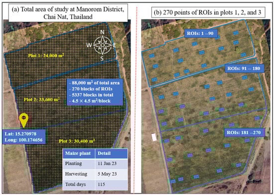
Figure 1.
Area of study located in (a) Manorom District, Chai Nat, Thailand, with Latitude: 15.270978, Longitude: 100.174656. (b) A total of 270 blocks of ROIs in Plots 1, 2, and 3 were selected for analysis.

Table 1.
Climate data for maize growth in the period of study of 11 January to 5 May 2013.
The primary objective of this study is to rigorously examine the productivity of crop yield within the three designated plots. By analyzing and assessing the agricultural output achieved in each plot, this investigation aims to provide valuable insights into the crop yield performance.
2.2. Unmanned Aerial Vehicle (UAV) Data Acquisition
The study employs the DJI Phantom 4 Multispectral (P4M) quadcopter, which is a drone equipped with multispectral imaging capabilities [], for capturing aerial images. The P4M quadcopter is equipped with six sensors, including an RGB sensor with 2.08 megapixels, a blue sensor (450 nm ± 16 nm), a green sensor (560 nm ± 16 nm), a red sensor (650 nm ± 16 nm), a red edge sensor (730 nm ± 16 nm), and a near-infrared sensor (840 nm ± 26 nm). These sensors enable the acquisition of comprehensive spectral information. The flight missions were conducted using the DJI GS Pro software version 2.0.17, with specific settings applied. The settings included a speed of 3.2 milliseconds, a shutter interval of 2 seconds, a front overlap ratio of 75%, a side overlap ratio of 75%, and a course angle of 119 degrees. The UAV was flown at altitudes of 30 m and 100 m to capture data from different perspectives. In order to mitigate the influence of varying sunlight angles, the UAV flights were scheduled between 10:00 a.m. and 12:00 p.m.
It is noteworthy that the maize growth stages are commonly delineated using a standardized system developed by the Food and Agriculture Organization (FAO). In the context of our research, it is of paramount importance to investigate and ascertain the potential correlations between specific growth stages and the width of maize seeds, employing an innovative and novel approach. To achieve this objective, we meticulously conducted weekly monitoring of maize growth utilizing UAVs. A total of 17 UAV flights were conducted over a comprehensive 113-day period, encompassing the entire growth cycle of the maize plants. The detailed data obtained from these flights are meticulously presented in Table 2, providing valuable insights for further analysis and interpretation.
Table 2.
Image acquisition by UAV flights.
During the Vegetative Stage (VE) of maize growth, which signifies the emergence of the first leaves, our UAV observation campaign was initiated on 11 January 2023. RGB and multispectral images were acquired during this phase, utilizing UAV flights conducted at altitudes of 30 m and 100 m. The purpose of these flights was to capture comprehensive data encompassing both standard RGB imagery and multispectral information regarding the early growth patterns of maize plants. Furthermore, on day 8 of maize growth, the emergence of leaves begins. By day 56, the plant typically reaches the stage where ten leaves have appeared.
In order to maintain optimal conditions for maize growth, it is crucial to address both excessive moisture and prolonged drought. These conditions have the potential to reduce the yield by up to 25% between the sixth leaf stage (V6), characterized by the development of six leaves with visible collars, and the tenth leaf stage (V10), characterized by the development of ten leaves with visible collars. To ensure the appropriate growth of maize, we consistently monitored its progress on a weekly basis across all growth stages. Additionally, during the transition from the V10 stage to the tasseling stage or Vegetative Tassel (VT), which involves the emergence of the tassel and the initiation of pollen shedding, the demand for nutrients and water increases significantly to meet the growth requirements. In response, we decided to implement precision fertilizer technology to optimize soil fertility. It is essential to be aware that the presence of insects and the occurrence of hail injuries during this critical stage can potentially reduce kernel production.
The silking stage (R1) is a crucial phase for determining maize grain yield. In our research, silks emerged and became receptive to pollen on day 65. Physiological maturity can be estimated by adding 50 to 55 days from the R1 stage. By day 72, we observed the blister stage (R2), characterized by the swelling and milky fluid filling of kernels, resembling blisters. This stage represents a significant milestone in maize development, marking the transition from vegetative growth to reproductive growth and the initiation of kernel development. It is important to note that drought conditions during the R2 stage can cause substantial yield reductions, ranging from 50% to 60% per day. Therefore, providing adequate nutrients and water during this stage is essential to support proper kernel development and maturation, ultimately influencing the final grain yield.
In our research, we observed the reproductive stage (R3) (milk stage) on day 85. This stage is characterized by the continued filling of kernels with a milky fluid, reaching their maximum size. The R3 stage plays a pivotal role in determining the potential yield of maize as it represents a critical period for kernel growth and development. Subsequently, during the reproductive stage (R4) (dough stage), significant changes occur as the kernels gain dry weight and size, acquiring a doughy consistency. The transition to the reproductive stage R5 (dough stage) was observed on day 99. At this stage, the kernels continue to develop, filling with a dough-like substance and transitioning from a milky appearance to a more solid texture. Finally, on day 113, the maize plant approached physiological maturity at the reproductive stage R6 (physiological maturity stage). At this stage, the kernels were in their late developmental phases, indicating the culmination of the growth process.
During all flights, Ground Control Points (GCPs) are captured and serve as reference points for the creation of image mosaics. This practice ensures consistency and enables effective comparison between images obtained on different dates. The resulting mosaic images possess a Ground Sampling Distance (GSD) of 0.016 m and 0.053 m when captured at flight altitudes of 30 m and 100 m, respectively. To maintain uniformity across all acquired images captured at various stages of growth, a series of processing steps were applied.
2.3. Image Processing for Extracting Twelve Vegetation Indices
The pre-processing of red, green, blue (RGB) and multispectral (MS) images was conducted using DJI Terra version 4.0.10, a photogrammetry software developed in Shenzhen, China. DJI Terra utilizes the RGB channels, along with near-infrared (NIR) and red edge channels at each wavelength, to perform image processing.
Figure 2 provides a visual representation of the entire process, offering a comprehensive overview of the processing steps involved in handling both RGB and MS images. These steps are specifically designed to extract digital traits, as adapted from [].
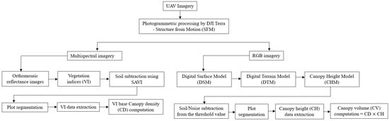
Figure 2.
Image processing pipelines for digital traits’ extraction adapted from []. From the multispectral (MS) images, twelve vegetation indices were generated. On the other hand, from the red, green, blue (RGB) images, twelve canopy volumes were obtained.
A comprehensive data collection effort was undertaken during the investigation, covering all three plots. This endeavor resulted in the acquisition of 3172 .tif files from each flight conducted at an altitude of 30 m and 835 .tif files from each flight conducted at an altitude of 100 m. Across a total of 17 flights, the dataset encompasses 53,924 .tif file images captured at an altitude of 30 m, along with an additional 14,195 “.tif” file images captured at an altitude of 100 m. The employed software, DJI Terra, utilizes advanced techniques such as scene illumination, reference panels, and sensor specifications to automatically generate orthomosaic images in .tif format from both datasets.
2.3.1. Vegetation Indices
In agricultural applications, twelve commonly used vegetation indices (VIs) are instrumental in assessing vegetation health and performance. These indices encompass a range of parameters and include: (1) Chlorophyll Index green (CIgr), (2) Chlorophyll Index red edge (CIre), (3) Enhanced Vegetation Index 2 (EVI2), (4) Green Normalized Difference Vegetation Index (GNDVI), (5) Modified Chlorophyll Absorption Ratio Index 2 (MCRI2), (6) Modified Triangular Vegetation Index 2 (MTVI2), (7) Normalized Difference Red Edge (NDRE), (8) Normalized Difference Vegetation Index (NDVI), (9) Normalized Difference Water Index (NDWI), (10) Optimized Soil-Adjusted Vegetation Index (OSAVI), (11) Renormalized Difference Vegetation Index (RDVI), and (12) Red–Green–Blue Vegetation Index (RGBVI), as shown in Table 3.
Table 3.
Vegetation indices formulations and references.
To mitigate the influence of soil surface on each VI image, a soil mask layer is generated using the soil-adjusted vegetation index. The plots are defined by 270 ROIs, each measuring 4.5 × 4.5 m, and are digitized in a shapefile (*.shp) format using the open-source software Quantum GIS (QGIS, version 3.28.3-Firenze).
Ground reference data obtained from the harvested area are utilized to estimate the canopy volume (CV) based on the subplot polygons. Subsequently, the plot segmentation shapefiles are imported into the developed algorithm. Various image features, including maximum (Max), average (Mean), sum, standard deviation, 95th percentile, 90th percentile, and 85th percentile (representing the highest data values extracted after eliminating 5%, 10%, and 15% of the data following the soil subtraction process from the VI images, respectively, denoted as 95P, 90P, and 85P), are computed for each subplot within each VI image. These features are calculated using the Python libraries NumPy and Rasterstats. During the plot segmentation creation process, the feature data are labeled and subsequently exported as a Comma-Separated Values (CSV) file.
2.3.2. Canopy Height Model from Digital Surface Model
The estimation of crop height within each subplot relies on the utilization of a Canopy Height Model (CHM) []. To create a Digital Terrain Model (DTM) representing the field’s topography, the QGIS software is employed. The CHM is obtained by subtracting the Digital Surface Model (DSM) data from the DTM. To ensure heightened accuracy, a filtering process is applied to the CHM image layer, eliminating pixels with a height below a predefined threshold of 0.05 m. Subsequently, the CHM image layer is segmented using a plot segmentation shapefile, enabling the extraction of statistical data for each individual ROI to acquire canopy height (CH) information. The calculation of canopy volume (CV) is performed by multiplying the data related to canopy density (CD) with the corresponding CH data for each specific ROI. This sequential process is carried out for all the ROIs investigated in the study, thereby obtaining the CV values.
2.4. Environmental Measurements and Optimal IoT Design for Soil Health Monitoring
In order to facilitate a comprehensive investigation of soil properties and environmental data, the authors integrated multiple sources of information to assess various aspects. As discussed in Section 2.2, UAVs were utilized, as depicted in Figure 3a. To enable comprehensive weather monitoring, a Vantage Pro2 weather station [] from Davis Instruments Corporation, Diablo Avenue Hayward, CA, USA, as shown in Figure 3b, was employed. The Vantage Pro2 is an agriculture-focused weather station that includes outside temperature and humidity, wind speed, rainfall, and solar radiation, plus a solar radiation sensor for evapotranspiration measurement. The sensor provides accurate, reliable weather monitoring with real-time data updates every 0.5 seconds. Our sensor network is designed to collect a wide range of environmental parameters, including, but not limited to light intensity, humidity, temperature, and precipitation. By capturing these variables, we ensured that our dataset encompasses diverse meteorological conditions, ranging from bright and sunny days to overcast or rainy weather. Furthermore, a series of measurements including NPK nutrient levels, pH, and Electrical Conductivity (EC) were obtained using the Soil Analyzer from Weihai JXCT Electronic Technology Co., Ltd., Weihai, China [], as illustrated in Figure 3c.
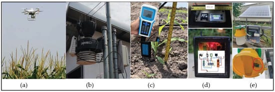
Figure 3.
Equipment used for the measurements in the research: (a) DJI Drone with multi-spectrum capability, (b) Vantage Pro2 weather station, (c) NPK Soil Analyzer, (d) our IoT design for soil health monitoring, and (e) prototype of smart trap.
The IoT devices specifically designed for measuring soil parameters such as pH, NPK levels, Electrical Conductivity (EC), moisture, and location were developed []. These devices utilize a low-power transmission technique known as Long-Range Wide-Area Network (LoRaWAN) to ensure efficient and reliable data transmission. The IoT-based soil monitoring system, as depicted in Figure 3d, incorporates these LoRaWAN-enabled devices. Additionally, the innovative smart trap for insect monitoring, showcased in Figure 3e, was proposed by the authors as a prototype system.
The IoT-based system for soil monitoring consists of an Arduino Nano, soil sensors, a 3.7 V 3000 mAh battery, and a Tiny GPS []. To enable wireless communication and achieve seamless data transmission over a range of approximately 2 km, the system utilizes the Gravitech S767 microcontroller from CAT Telecom, National Telecom Public Company Limited, Lak Si, Bangkok, Thailand, produced in Thailand, which implements the LoRaWAN. The microcontroller Arduino Nano version 3.0 from Arduino LLC, Somerville, MA, USA interfaces with the soil sensors using RS485 communication. The IoT devices are programmed to send and retrieve data at five-minute intervals over a period of seven days.
In this study, the authors primarily utilized the innovative smart trap for insect monitoring and insect counting. The smart trap employs a Raspberry Pi controller and advanced object-detection techniques, specifically YOLOv5. This integration enables real-time decision making in precision agriculture, with the aim of minimizing chemical usage, promoting sustainable crop protection, and optimizing crop yield and quality. This integration serves the purpose of fostering a future marked by sustainable and productive farming practices.
2.5. Selection of Machine Learning (ML) Methods for Grain Yield Predictions
In the domain of machine learning (ML) in precision agriculture, the authors present a comprehensive approach, as illustrated in Figure 4, to identify the most suitable model for crop yield prediction. The study explores the efficacy of 14 distinct ML algorithms in predicting the growth stage and productivity of maize. These algorithms encompass CatBoost regression [], decision tree regression [,], ElasticNet regression [], gradient boosting regression [,], Huber regression [], K-Nearest Neighbors (KNN) regression [], LASSO regression [], linear regression [], M estimators [], passive aggressive regression, random forest (RF) regression [], ridge regression, Support Vector Regression (SVR) [], and XGBoost regression []. By employing this diverse range of algorithms, the authors aimed to optimize the accuracy and reliability of crop yield prediction in the context of precision agriculture.
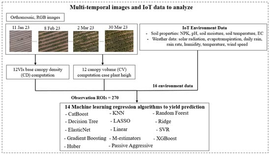
Figure 4.
The flow diagram of ML methods for grain yield prediction.
The proposed flow chart encompasses two integral components. The first component involves the analysis of multi-temporal images, as explicated in Section 2.3, wherein a comprehensive examination is conducted on various vegetation indices, chlorophyll contents, and other pertinent features. A total of 17 imagery datasets, acquired from 17 flights, as delineated in Table 2, underwent meticulous scrutiny, resulting in the extraction of 4590 ROIs derived from the multiplication of 270 ROIs by 17 days. These carefully selected ROIs were seamlessly integrated with 14,195 .tiff images utilizing the DJI Terra software version V4.0.10, thereby establishing pixel-to-ROI correspondences. The ROIs were subjected to rigorous processing, incorporating precise geographic coordinates obtained through Ground Control Points (GCPs) following established procedures. The extracted pixel data derived from these ROIs serve as the fundamental basis for computing VI-based canopy density, thereby enabling the classification of pixels into two distinct categories—green pixels and non-green pixels. By focusing exclusively on green pixels, the values of twelve VIs were computed for each ROI.
The computed VIs were subsequently employed to establish linear relationships with maize yields, aiming to investigate their correlation. Specifically, the VIs obtained during critical growth stages were utilized to calculate the coefficient of determination (R-squared, R2) values. These R2 values serve as indicators of the predictive capabilities exhibited by the various vegetation indices. By identifying the most effective indices during significant growth stages, valuable insights can be gained regarding growth monitoring, and more accurate yield predictions can be made.
The second part of the flow chart focuses on the application of ML algorithms for crop yield prediction. Over the past decade, ML algorithms have demonstrated remarkable potential and have outperformed traditional methods in various domains, including object detection, image classification, pattern recognition, and others. Leveraging supervised learning techniques, these algorithms have proven to be highly effective. In the specific context of crop yield prediction, the trained ML models were evaluated by assessing their performance on independent test samples. To select the most suitable ML algorithm for crop yield prediction, a careful selection process was undertaken. This involved considering a range of 14 ML algorithms, chosen based on their prominence in the literature and their distinctive characteristics. The goal was to identify the algorithm that best aligns with the specific requirements of predicting the growth stage and productivity of maize.
To investigate the effectiveness of ML models, this study utilizes a set of twelve VIs based on the CD. These VIs were computed from a long-term series of collected images for each plot. The VIs were employed as independent variables, while the maize yields observed in each plot were utilized as dependent variables.
This investigation made use of a diverse range of meticulously selected ML algorithms. The selection process took into consideration the distinctive characteristics of each algorithm, as well as insights derived from the relevant academic literature. The primary goal was to conduct a comprehensive analysis of multi-temporal satellite imagery data in order to provide accurate predictions of crop yields. Each chosen model underwent careful evaluation to ensure its suitability for the specific task at hand.
Model 1 (CatBoost regression) []: This algorithm was chosen for its adeptness in handling categorical features prevalent in such data. By employing ordered boosting and symmetric trees, CatBoost effectively captured temporal variations and seasonality patterns, ensuring a high level of predictive accuracy.
Model 2 (decision tree regression) [,]: Selected to interpret the impact of different temporal features on crop yields, decision tree regression leverages its hierarchical structure to represent complex relationships within the data.
Model 3 (ElasticNet regression) []: Addressing multicollinearity and performing feature selection simultaneously, ElasticNet regression has proven crucial for high-dimensional multi-temporal data. Its combination of L1 and L2 regularization techniques played a pivotal role in achieving these objectives.
Model 4 (gradient boosting regression) [,]: Demonstrating efficacy in handling complex relationships and temporal dependencies, gradient boosting regression build an ensemble of decision trees sequentially, enhancing predictive accuracy in the process.
Model 5 (Huber regression) []: Chosen for its robustness in accommodating outliers prevalent in agricultural datasets, Huber regression minimizes the impact of extreme values through a parameter balancing the mean absolute error (MAE) and mean-squared error (MSE).
Model 6 (K-Nearest Neighbors regression) []: Predicting grain yields based on similar multi-temporal patterns observed in the past, KNN regression relied on the assumption that analogous temporal patterns yield similar crop yields. However, the consideration of an appropriate K value and computational cost for larger datasets was warranted.
Model 7 (LASSO regression) []: Serving as a feature selection technique, LASSO regression incorporates L1 regularization to encourage some feature coefficients to be precisely zero, facilitating the identification of vital temporal features.
Model 8 (linear regression) []: Providing a baseline model to understand the overall trend between crop yields and multi-temporal features, linear regression assumed a linear relationship, offering valuable insights into the general temporal trend of grain yield.
Model 9 (M estimators regression) []: Chosen for their robustness in handling outliers and noise in agricultural datasets, M estimators provided flexibility in choosing the loss function, making them suitable for data with non-Gaussian noise.
Model 10 (passive aggressive regression): As an online learning algorithm, passive aggressive regression adapted quickly to temporal changes in crop yield patterns, making it suitable for real-time predictions, particularly in rapidly evolving agricultural conditions.
Model 11 (random forest regression) []: Handling high-dimensional multi-temporal data, RF provided robust predictions by building multiple decision trees on different data subsets and averaging their predictions.
Model 12 (ridge regression): Beneficial when dealing with multicollinear features in multi-temporal data, ridge regression applied L2 regularization to stabilize the model and reduce the impact of multicollinearity.
Model 13 (Support Vector Regression) []: Chosen for its capability to capture non-linear relationships between multi-temporal features and crop yields, SVR mapped data into a higher-dimensional space, enabling the identification of non-linear patterns.
Model 14 (XGBoost regression) []: Selected for its effectiveness in various regression tasks, XGBoost regression constructed an ensemble of decision trees using gradient boosting and regularization techniques, offering high predictive accuracy.
These ML algorithms were amalgamated to form a comprehensive toolkit capable of analyzing multi-temporal satellite imagery data and accurately predicting crop yields. Through their collective usage, they effectively addressed various challenges encountered in the analysis process, including outlier handling, feature selection, non-linearity, and temporal dependencies.
2.6. Selection of Best Suited Models
The selection of the most appropriate models depends on the specific characteristics of the multi-temporal imagery and the nature of the grain yield data. Models such as CatBoost regression and gradient boosting regression are well suited to capturing temporal patterns and seasonality effects. ElasticNet and LASSO regression offer valuable features for feature selection in high-dimensional data. Huber regression and M estimators are effective at handling outliers within the crop yield data. Given the diverse range of scenarios and variable combinations explored in this study, it is crucial for researchers to rigorously evaluate each algorithm’s performance using defined evaluation metrics. This meticulous evaluation process enables researchers to identify the most effective models for accurately predicting grain yield within their unique agricultural context, thus enhancing the reliability and accuracy of the predictions.
To evaluate the performance of these various algorithms [,,,], the authors used several metrics, including mean-squared error (MSE), root-mean-squared error (RMSE), mean absolute error (MAE), and R-squared () as
and
where N is the number of all samples, M and P are the true values and predicted values of the yields, represents the actual values, represents the predicted values, represents the absolute value, and represents the mean of the actual values, respectively. These metrics provide insights into the accuracy and predictive power of each algorithm in estimating the growth stage and productivity of maize.
The study encompasses an extensive set of forty features utilized as inputs for the ML models to facilitate the accurate prediction of crop growth and yield. This comprehensive set of features comprises eight soil-related factors, eight parameters derived from environmental data, and twenty-four features derived from twelve VIs. The soil-related factors encompass N, P, K, pH level, soil temperature, soil humidity, EC, and maize height. These factors provide insights into the soil composition, fertility, and moisture content, as well as the growth status of the maize plants. On the other hand, the parameters derived from environmental data capture important variables such as water feed, UV radiation, evapotranspiration, daily rainfall, rain rate, humidity, wind speed, and temperature. These environmental factors play a crucial role in influencing crop growth and yield, and their inclusion in the analysis allows for a comprehensive understanding of the interactions between soil conditions and the surrounding environment.
Furthermore, the study incorporates twenty-four features derived from twelve VIs, specifically the CIgr, CIre, EVI2, GNDVI, MCARI2, MTVI2, NDRE, NDVI, NDWI, OSAVI, RDVI, and RGBVI, accompanied by the CD and CV. Through the incorporation of a diverse set of forty features, ML models can capture the complex relationships between soil properties, environmental conditions, and vegetation characteristics, thereby exerting a significant influence on crop health and a holistic analysis of crop growth and productivity.
2.7. Ensemble Model for Improved Grain Yield Predictions
This section presents an ensemble machine learning (ML) model designed to enhance the accuracy and reliability of grain yield predictions by harnessing the strengths of multiple individual models. Ensemble models have emerged as a prominent technique in agricultural data analysis due to their capacity to mitigate limitations and improve accuracy by effectively capturing diverse patterns and relationships in the data. By combining the predictive power of multiple ML algorithms, the ensemble model contributes to more robust and accurate grain yield predictions.
Within our ensemble model, we meticulously selected a range of top-performing machine learning (ML) algorithms, including Huber regression, M estimators, linear regression, ridge regression, and others, based on their demonstrated effectiveness in capturing temporal variations, addressing multicollinearity, and accommodating outliers present in the dataset.
The operational framework of the ensemble model is structured as follows:
- Data preparation: To combine the data from various sources, we collected the following:
- -
- Twenty-four VIs with the CD and CV (CIgr, CIre, EVI2, GNDVI, MCARI2, MTVI2, NDRE, NDVI, NDWI, OSAVI, RDVI, and RGBVI).
- -
- Sixteen environmental data (maize height, N, P, K, pH, soil temperature, soil humidity, EC, water feed, UV radiation, evapotranspiration, daily rain, rain rate, humidity, wind speed, temperature).
In summary, we have forty features with two hundred seventy data plots on each of the seventeen dates to process, with in total 137,700 records from the dataset. In addition, data cleaning, missing value handling, and null entry removal were also included:
- Feature engineering: Use six different feature importance techniques to extract significant features:
- -
- Random forest importance consists of a large number of individual decision trees that operate as an ensemble. Each individual tree in the random forest outputs a class prediction, and the class with the most votes becomes the model prediction. The importance of each feature is determined by the average impurity decrease calculated from all decision trees in the forest.
- -
- Recursive feature elimination (RFE) with cross-validation is a method that fits the model multiple times, and at each step, it removes the weakest feature (or features). RFE with cross-validation uses the cross-validation approach to find the optimal number of features.
- -
- Permutation importance can be used with any model. After a model is trained, the values in a single column of the validation data are randomly shuffled. Then, the model performance metric (such as accuracy or ) is re-evaluated with the shuffled data. Features that have a significant impact on performance are considered important.
- -
- LASSO regression coefficients is a regression analysis method that performs both variable selection and regularization to enhance the prediction accuracy and interpretability of the statistical model. LASSO selects features with non-zero coefficients.
- -
- The correlation coefficient measures the linear relationship between the target and the numerical features. Features that have a higher correlation with the target variable are considered important.
- -
- SHapley Additive exPlanations (SHAP) is a unified measure of feature importance. It assigns each feature an important value for a particular prediction.
- Model selection: We meticulously evaluated the performance of various ML algorithms on our grain yield prediction task. The top arbitrary number models, based on evaluation metrics such as mean-squared error (MSE), root-mean-squared error (RMSE), mean absolute error (MAE), and R-squared (), were chosen for ensemble construction.
- Training: Each of the selected models was trained on our dataset, utilizing the same training, testing, and validation splits of 70%, 20%, and 10%, respectively, to ensure consistency and fairness in the comparison. Fourteen different ML models were trained and evaluated for the data. The models included the following:
- -
- CatBoost, decision trees, ElasticNet, gradient boosting, Huber, KNN, LASSO regression, linear regression, M estimators, passive aggressive, RF, ridge regression, SVR and XGBoost.
- Ensemble building: We created the ensemble by combining the predictions of the top arbitrary models using weighted averaging. The weights assigned to each model were determined based on their performance during training. This process optimizes the ensemble’s predictive accuracy. The weighted ensemble prediction is given bywhere , , and represent the weights assigned to each model and , , and are the predictions made by each individual model. We fine-tuned the weights (denoted as , , and ) based on the preliminary evaluation results, exploring various weight combinations to optimize the ensemble model’s performance.
- Evaluation: The ensemble model’s performance was evaluated using the same evaluation metrics employed for individual models. We compared its results to those of individual models to gauge the improvement achieved through ensemble modeling.
- Hyperparameter tuning: If necessary, we fine-tuned the hyperparameters of our ensemble model to enhance its predictive capabilities further. Techniques such as grid search or random search were employed for this purpose.
By incorporating the ensemble model into our grain yield prediction framework, we aimed to provide more accurate and reliable forecasts, ultimately assisting farmers and agronomists in optimizing crop management practices and decision making in precision agriculture. The fusion of multiple ML algorithms within the ensemble harnesses the strengths of each model, resulting in a robust tool for agricultural yield predictions.
3. Results
Through a comprehensive analysis of environmental factors and various vegetation indexes, this study aims to determine which aspects of the maize growth stage and other factors can be adjusted to predict seed weight. In the first part of the study, a total of seventeen UAV flights were conducted to collect images from a bird’s-eye view, creating a detailed map of the study area. The images’ data from each day were then computed for twenty-four vegetation indexes with both the CD and CV, namely the CIgr_CD, CIre_CD, EVI2_CD, GNDVI_CD, MCAR2_CD, MTVI2_CD, NDRE_CD, NDVI_CD, NDWI_CD, OSAVI_CD, RDVI_CD, RGBVI_CV, CIgr_CV, CIre_CV, EVI2_CV, GNDVI_CV, MCAR2_CV, MTVI2_CV, NDRE_CV, NDVI_CV, NDWI_CV, OSAVI_CV, RDVI_CV, and RGBVI_CD.
The goal was to identify which specific days of the growth stage and vegetation indexes show high correlations with seed weight. The results are presented in Figure 5, which highlights five dates and five vegetation indexes (VIs) that displayed a strong correlation with seed weight. These included day 56 of stage V10, days 65 and 72 of stage R1, and day 79 of stage R2, and day 85 of stage R3. Additionally, the VIs with the highest correlation were the CIre_CD, NDRE, CIgr, EVI2, and NDVI. Notably, on day 79 of stage R2, the VI indexes CIre, NDRE, CIgr, EVI2, and NDVI demonstrated particularly high correlations of 0.80, 0.80, 0.77, 0.75, and 0.74, respectively. Forty features with two hundred seventy data plots on day 79 of stage R2 were selected to feed the ML algorithm to predict grain yield.
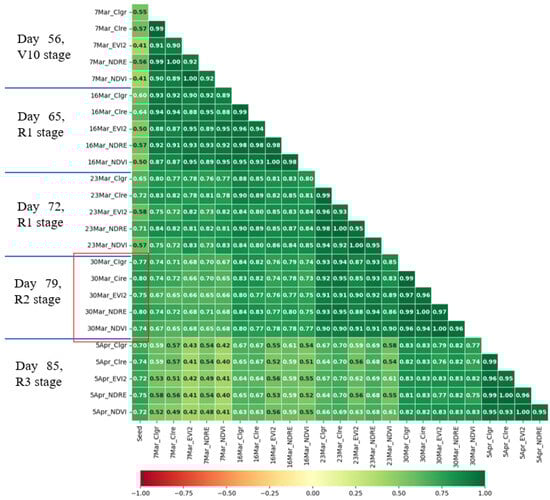
Figure 5.
Five high correlation of date of growth stage and VIs with seed weight. Green shades indicate positive correlations, darker shades suggest stronger relationships, red shades suggest negative correlations, darker shades suggest stronger inverse relationships, and neutral shades indicate little to no correlation.
In this study, all ground truth data were gathered simultaneously on a singular date and time during the unmanned aerial vehicle (UAV) flight missions. The collected data were bifurcated into two distinct categories: the first encompassing the soil properties’ data, which entailed NPK nutrient levels, pH, EC, soil temperature, soil humidity, water feed per area (m3/dunam), and maize height (m) and the second comprising weather data, including ultraviolet radiation (UV), evapotranspiration, daily rain, rain rate, humidity, wind speed, and temperature. The weather-related data were consistently captured at five-minute intervals throughout the entire growing season.
Figure 6 depicts the correlation between seed weight and sixteen factors derived from the soil properties and weather data used for the analysis. Daily rain and rain rate were excluded from this correlation analysis due to their predominantly negligible values throughout the entire growing season, with most observations indicating zero or minimal rainfall. Among the various factors examined, several displayed a modest correlation with seed weight. These factors encompassed maize height, temperature, humidity, wind speed, UV radiation, water feed, and evapotranspiration, exhibiting correlation coefficients of 0.32, 0.28, 0.26, 0.25, 0.19, 0.19, and 0.17, respectively.
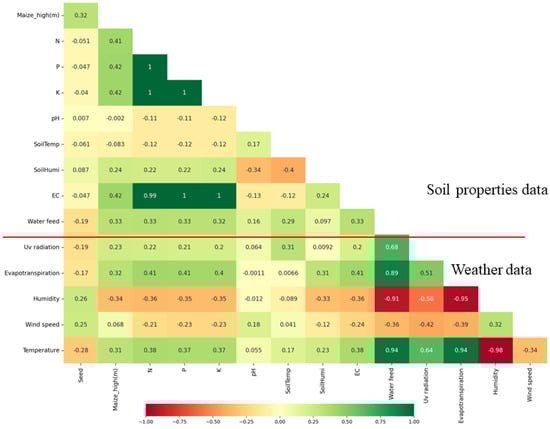
Figure 6.
Sixteen environment data to correlate with seed weight. For the daily rain and rain rate, the values are zero and do not appear in correlation chart. Green shades indicate positive correlations, darker shades suggest stronger relationships, red shades suggest negative correlations, darker shades suggest stronger inverse relationships, and neutral shades indicate little to no correlation.
To facilitate the analysis, the weather data obtained on day 79, corresponding to stage R2 or 30 March 2023, during the time interval from 10.00 a.m. to 2.00 p.m., were averaged. These weather data were collected using Internet of Things (IoT) sensors and included measurements of the temperature (39 °C), rainfall (0.0 mm), UV index (7.2 UV), and evapotranspiration rate (4.8 mm). Evapotranspiration refers to the movement of water from the land surface to the atmosphere through the processes of evaporation and transpiration, as depicted in Figure 7.
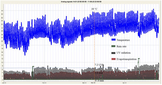
Figure 7.
The environment data of temperature, rain rate, UV radiation, and evapotranspiration of the day of prediction on 30 March 2023.
3.1. Best Suited Model Selection for Maize Grain Yield Prediction
This experiment is geared towards predicting maize grain yield by utilizing multi-temporal imagery to extract vegetation indices (VIs) based on the canopy density (CD) and canopy volume (CV), derived from the product of the canopy density and plant height. The analysis incorporates ground truth environmental data (Env), encompassing NPK nutrient levels, pH, EC, soil temperature, soil humidity, water feed per area (m3/dunam), and maize height (m). Additionally, weather data such as ultraviolet radiation (UV), evapotranspiration, daily rain, rain rate, humidity, wind speed, and temperature were considered.
On day 79 (30 March 2023) of stage R2, we identified the CIre, NDRE, CIgr, EVI2, and NDVI, determining which days of the growth stage and vegetation indices were highly correlated with the target variable and can be effectively utilized for prediction in our research.
To contribute to the understanding of our methodology, the authors provide the ensemble ML model pipeline, as depicted in Figure 8.
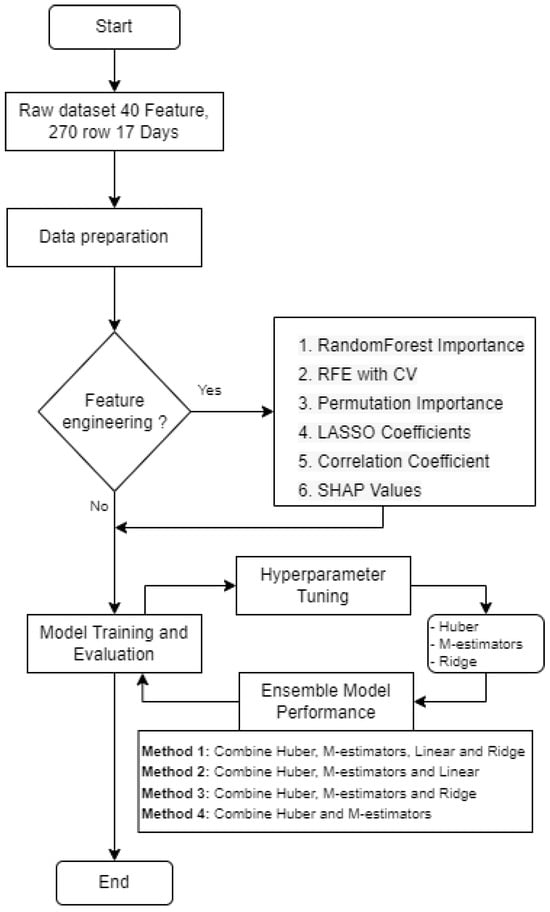
Figure 8.
Ensemble pipeline for our purposes.
The initial phase of this study involved meticulous data preparation, where the dataset underwent thorough collection, and cleaning procedures were implemented to address missing values and eliminate null entries.
Subsequently, in the feature-engineering stage, six distinct techniques were applied to extract significant features. These methods encompassed selecting all 40 features (excluding the target for predicting “seed”), utilizing random forest importance to identify features like the “CIre_CD”, “NDRE_CD”, “CIgr_CD”, “EVI2_CD”, and “NDVI_CD”, employing recursive feature elimination with cross-validation (RFE with CV) to highlight features such as “CIre_CD”, “NDRE_CD”, “CIgr_CD”, “EVI2_CD”, and “NDVI_CV” and utilizing permutation importance to pinpoint features like “CIre_CD”, “NDRE_CD”, “CIgr_CD”, and “EVI2_CD”. Additionally, features were selected based on the LASSO coefficients (“CIgr_CD”, “CIgr_CV”, “SoilHumi”, “wind speed”), the correlation coefficient (“NDRE_CD”, “evapotranspiration”, “humidity”, “temperature”, “EC”), and the SHAP values (“CIre_CD”, “NDRE_CD”).
Following feature engineering, the study progressed to model training and evaluation, employing a diverse set of fourteen ML models, CatBoost, decision tree, ElasticNet, gradient boosting, Huber, KNN, LASSO regression, linear, M estimators, passive aggressive, RF, ridge, SVR, and XGBoost regression.
Hyperparameter tuning was then conducted to optimize specific models, namely “Huber”, “M estimators”, “linear regression”, and “ridge regression”. This fine-tuning process utilized GridSearchCV to identify and implement the most effective hyperparameters for enhanced model performance.
Finally, the study explored ensemble techniques to amalgamate the predictions from multiple models, thereby improving overall performance. Four distinct ensemble methods, labeled PEnsemble1, PEnsemble2, PEnsemble3, and PEnsemble4, were implemented, combining various models such as “Huber”, “M estimators”, “linear regression”, and “ridge regression” in different configurations to leverage the strengths of individual models and enhance predictive accuracy.
To determine the most suitable model prior to employing ensemble techniques, the authors adopted six distinct methods of feature engineering:
- Random forest importance: This method leverages the random forest algorithm, which constructs a multitude of decision trees during training. The importance of a feature is computed by observing how often a feature is used to split the data and how much it improves the model’s performance.
- Recursive feature elimination (RFE) with cross-validation: RFE is a technique that works by recursively removing the least important feature and building a model on the remaining features. The process is repeated until the desired number of features is achieved. Cross-validation is integrated into this process to optimize the number of features and prevent overfitting.
- Permutation importance: This technique gauges the importance of a feature by evaluating the decrease in a model’s performance when the feature’s values are randomly shuffled. A significant drop in performance indicates high feature importance.
- LASSO regression coefficients: LASSO is a regression analysis method that uses L1 regularization. It has the capability to shrink some regression coefficients to zero, effectively selecting more significant features while eliminating the less impactful ones.
- Correlation coefficient: This method calculates the linear correlation between each feature and the target variable. Features that have strong correlation coefficients are deemed important, as they have a substantial linear association with the target.
- SHAP values: SHAP values furnish a metric for gauging the influence of each feature on the model’s prediction. By attributing the difference between the prediction and the average prediction to each feature, SHAP provides a more intuitive comprehension of feature importance, particularly in the context of complex models.
The study employed six different feature engineering techniques to prioritize the selection of features based on their importance, ensuring the utilization of the most significant predictors in the model. Table 4 and Table 5 present the performance of various ML models across these distinct feature engineering methods.
Table 4.
Top 10 best performances of fourteen ML model across six distinct methods of feature engineering.
Table 5.
Top 10 worst performances of fourteen ML model across six distinct methods of feature engineering.
Among the top-performing models, the Huber model stands out, achieving the best value of 0.926313 with features selected using SHAP values. This combination demonstrates minimal errors with an MAE of 0.278809, an MSE of 0.516539, and an RMSE of 0.718707, explaining approximately 92.63% of the variance in the dependent variable. The Huber model, when paired with features selected using the correlation coefficient, permutation importance, random forest importance, and RFE with CV, consistently maintains values exceeding 92.63%, indicating its robust performance. The M estimators model, coupled with features selected using SHAP values and permutation importance, also showcases strong performance with an value above 92.46%.
Conversely, the top 10 worst performing models include the decision tree model with features selected using all features, permutation importance, and LASSO coefficients, exhibiting values below 43%. This suggests potential overfitting to the training data or the decision tree model’s limited suitability for the dataset. The passive aggressive model, using the correlation coefficient feature selection method, and the ElasticNet model, utilizing both correlation coefficient and LASSO coefficients, also present low values, indicating weaker performance. The XGBoost model with features selected using SHAP values and the decision tree model with features selected using RFE with CV both have values below 65%, further suggesting challenges with these combinations.
In summary, the results highlight that the Huber model consistently demonstrates strong performance across multiple feature-selection methods, indicating its suitability for this dataset and problem. Conversely, the decision tree model appears less suited, producing some of the lowest values, suggesting it might not be the optimal choice or may require further refinement through hyperparameter tuning or constraints to prevent overfitting. The study also underscores the effectiveness of feature-selection methods such as SHAP values, correlation coefficient, permutation importance, random forest importance, and RFE with CV, particularly when combined with the Huber model.
Consequently, Huber, M estimators, ridge regression, and linear regression were selected from six different feature importance techniques for further processing with the hyperparameter tuning technique—an essential step in the ML workflow. The primary objective was to search for the optimal combination of hyperparameters that yields the best model performance.
The GridSearchCV method facilitates an exhaustive search over a specified parameter grid, employing cross-validation to estimate the performance of each combination. For the Huber model, the best parameter tuning resulted in an achieved of 0.926266, setting the regularization strength () to 1, the Huber threshold () to 1.0, and the maximum number of iterations (max_iter) to 100.
For the parameters of M estimators within the RANSACRegressor algorithm, the minimum number of samples (min_samples) was set to 0.7 of randomly available data samples for each iteration, and the stop-iterating probability (stop_probability) was set to 0.9. The obtained of 0.924029 was achieved when 70% of the samples were used to fit the model in each iteration, and the algorithm iterated until there was a 96% probability of correctly identifying the inliers.
The linear regression model, configured with fit_intercept=True, enhances flexibility, allowing it to better capture data patterns, resulting in an achieved of 0.918301. Fine-tuning the parameters of the ridge regression model involved setting the alpha to 0.615848211066026, fit_intercept to True, and selecting “lsqr” as the solver. The “lsqr” solver, representing “Least Squares QR Decomposition”, proves efficient in solving the least squares problem. The ridge regression model yielded the best score of 0.916892 when the regularization strength was 0.615848211066026, an intercept was included, and the lsqr solver computed the coefficients. A summarized overview of the hyperparameter tuning results is presented in Table 6.
Table 6.
Summary of hyperparameters.
3.2. Results of Ensemble Models
In this subsection, we delve into the outcomes of our top-three ensemble models designed for predicting maize grain yield. These ensembles, meticulously curated by harnessing the strengths of various ML algorithms, underwent a comprehensive evaluation based on predefined performance metrics like the MSE, RMSE, MAE, and . Our analysis provides a detailed examination of each ensemble model’s precision and effectiveness in capturing intricate connections within multi-temporal satellite imagery data, environmental variables, and maize yields. Additionally, we conducted a comparative assessment to identify the top-performing ensemble, characterized by its accuracy and reliability in predicting grain yields.
Our presentation of these findings aims to offer valuable insights into the potential of ensemble modeling for maize grain yield prediction. We believe that such insights can prove instrumental for decision makers in agriculture and precision farming, guiding them toward more informed practices and strategies.
Following thorough feature engineering and hyperparameter tuning, our results highlight the effectiveness of the Huber, M estimators, ridge regression, and linear regression models when paired with the features “CIre_CD” and “NDRE_CD” derived from the SHAP values technique for predicting maize grain yield. Building on these findings, we opted to utilize the VotingRegressor to create ensembles for each method, thereby enhancing the predictive capabilities of our model as follows:
- PEnsemble 1: Using Huber, M estimators (RANSAC), linear regression, and ridge regression, the weighted ensemble prediction is given by
- PEnsemble 2: Using Huber, M estimators (RANSAC), and linear regression, the weighted ensemble prediction is given by
- PEnsemble 3: Using Huber, M estimators (RANSAC), and ridge regression, the weighted ensemble prediction is given by
- PEnsemble 4: Using Huber and M estimators (RANSAC), the weighted ensemble prediction is given by
The results, reflecting the weights assigned to each model in the ensemble methods, are presented in Table 7.
Table 7.
Evaluation metrics for different ensemble methods and Graph Neural Networks (GNNs) with the Graph Convolutional Network (GCN) and Graph Attention Network (GAN).
Method 1 (PEnsemble1) employs four distinct models: Huber, M estimators, linear regression, and ridge regression, each assigned weights of 0.5, 0.3, 0.1, and 0.1, respectively. The Huber model is granted the highest weight, emphasizing its substantial impact on ensemble prediction. This aligns with the robust nature of Huber’s regression, particularly beneficial in datasets susceptible to outliers. The obtained score was 0.924202, signifying commendable predictive performance.
In Method 2 (PEnsemble2), three models—Huber, M estimators, and linear regression—were included, with weights of 0.45, 0.35, and 0.2, respectively. Huber remains dominant, though to a lesser extent than in Method 1. The increased weight assigned to M estimators suggests a more balanced reliance on the robustness of both Huber and M estimators. The resulting score was 0.924131, slightly lower than Method 1, but still impressive.
Method 3 (PEnsemble3) utilizes three models—Huber, M estimators, and ridge regression—with weights of 0.45, 0.35, and 0.2, respectively. Similar to Method 2 in terms of weights, it substitutes linear regression with ridge regression. Ridge regression introduces L2 regularization, potentially preventing overfitting and enhancing generalization. However, the score was 0.924017, slightly lower than the scores obtained by the previous two methods.
Method 4 (PEnsemble4) employs only two models—Huber and M estimators—with weights of 0.6 and 0.4, respectively. Despite its simplicity, this ensemble heavily relies on the Huber model and achieved the highest score of 0.925427 among all methods. This result suggests that, at times, using fewer models with appropriate weighting can lead to superior predictions.
In summary, the results indicate that, while all ensemble methods exhibit robust performance, PEnsemble4 stands out for its superior prediction quality. The pronounced reliance on the Huber model, renowned for its resilience to outliers, is a crucial factor contributing to this exceptional performance. It is essential to recognize that the efficacy of ensemble methods can be contingent on the quality and characteristics of the data. Consequently, diverse datasets or varying feature sets may lead to divergent outcomes.
On the other hand, the authors conducted a comparative study to benchmark current ensemble machine learning methods with novel ones in other domains, such as deep learning, to predict crop yield. Prediction of corn variety yield with missing attribute data can be effectively addressed using Graph Neural Networks (GNNs) []. The result of Table 7 shows much worse performance, with Graph Convolutional Networks (GCNs), −0.057997 and Graph Attention Networks (GATs), −0.259505 having negative values, which means that these models perform worse than a mean baseline. This significant discrepancy may stem from the GNNs’ inability to capture the variance in the dependent variables effectively, or it may be due to issues related to overfitting or underfitting. The performance matrix of the study that compares GNNs to traditional ensemble machine learning methods showed a big difference in how well the models worked and how accurate the predictions were. The ensemble methods, PEnsemble1, PEnsemble2, PEnsemble3, and PEnsemble4, all had high values above 0.92, which means they had a strong predictive relationship. These ensemble methods leverage combinations of the Huber, M estimators, linear regression, and ridge regression models, contributing to their robust performance.
In summarizing the methodology employed in this study to predict maize yield using an ensemble ML model with IoT environmental data and UAV vegetation indices, we focused on assessing the performance of diverse models through various approaches to feature selection, hyperparameter tuning, and ensembling. The comparative evaluation of the scores for different models and methods is presented in Table 8 and Figure 9.
Table 8.
Comparison of scores for different models.
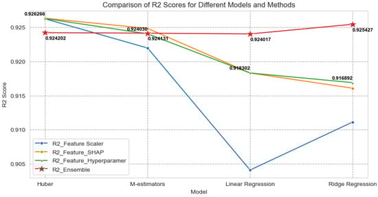
Figure 9.
Comparison of scores for different models and ensemble methods.
For feature scaling, the feature scaler utilized the StandardScaler to scale the training and testing datasets, standardizing them to have a mean of 0 and a standard deviation of 1. This process ensures that all features have the same scale, which is crucial for certain algorithms sensitive to feature scaling.
Feature importance, evaluated through the feature SHAP, involved employing SHAP to understand the importance of features in the model. SHAP provides a unified measure of feature importance, aiding in understanding which features the model deems significant.
Hyperparameter tuning, denoted as the feature hyperparameter, involved fine-tuning the model’s hyperparameters using GridSearchCV. This step ensures the selection of the best set of hyperparameters for the model, optimizing its performance.
In the ensembling phase, labeled as the ensemble, the models were combined using four different methods and weights. PEnsemble 1 combined Huber, M estimators, linear regression, and ridge regression with weights of [0.5, 0.3, 0.1, 0.1], resulting in an score of 0.924202. PEnsemble 2 combined Huber, M estimators, and linear regression with weights of [0.45, 0.35, 0.2], resulting in an score of 0.924131. PEnsemble 3 combined Huber, M estimators, and ridge regression with weights of [0.45, 0.35, 0.2], resulting in an score of 0.924017. PEnsemble 4 combined Huber and M estimators with weights of [0.6, 0.4], achieving the highest score of 0.925427.
In summary, the use of different strategies yielded diverse scores. Through ensembling, the strengths of individual models were effectively combined, potentially leading to improved and more robust predictions. Notably, the results indicate that the ensemble method, particularly Method 4 (incorporating Huber and M estimators), achieved a slightly superior score compared to the other ensemble methods and individual models. Importantly, the ensemble model demonstrated robustness in handling unseen data, enhancing its utility for predictive tasks.
In the context of our study, the accuracy of our model, validated with previously unseen data on the number of subgrids to coverage in each plot, is visually presented in Figure 10b. Plot 1, Plot 2, and Plot 3 comprise 1393 grids, 1612 grids, and 1693 grids, respectively. Figure 10a illustrates the accuracy trends of various prediction models across these distinct plots, encompassing both traditional and ML methodologies.
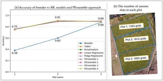
Figure 10.
(a) Accuracy of different ML model and PEnsemble approach vs. breeder and (b) the number of unseen data to predict grain yield.
- Breeder (traditional method): Our traditional approach exhibited varying accuracy levels across plots, with the lowest accuracy observed in Plot 1 and higher accuracies in Plots 2 and 3. Notably, it appears less effective for Plot 1, indicating potential limitations when predicting yields for certain scenarios.
- ML models (Huber, M estimators, linear regression, ridge regression): These models consistently demonstrated a stable accuracy range of 75–90% across all three plots. Linear regression and ridge regression, in particular, closely mirrored each other regarding predictive accuracy.
- PEnsemble approaches: Our ensemble methods (PEnsemble 1 to 4) showcased accuracies akin to individual ML models. Noteworthy is PEnsemble 4, exhibiting slightly superior performance across all plots, suggesting an effective amalgamation of the strengths of individual models.
In summary, the traditional “breeder” approach exhibited varied performance across plots, notably with lower accuracy in Plot 1. Additionally, the ML models, overall, presented more consistent and higher accuracy across all plots compared to the traditional method. In particular, PEnsemble 4 stood out marginally, underscoring its potential as a practical ensemble approach for maize yield prediction. This analysis suggests that ML models, especially ensemble methods, can be potent tools for predicting maize yields with higher accuracy than traditional methods, particularly in scenarios where the conventional approach might encounter challenges.
4. Discussion
4.1. Validating the Model with Unseen Data
In practical terms, the conventional breeder’s approach to yield prediction involves random sampling, as illustrated for each plot in Table 9.
Table 9.
Collection of ground truth data for maize plants using the traditional approach.
For Plot 1, covering an area of 24,000 m2 and hosting 8960 maize plants, a sampled cob contained 360 seeds. The weight of 100 seeds was 26 g, and the entire cob weighed 93.6 g. This translates to 3846 seeds per kilogram. Moving on to Plot 2, spanning 33,600 m2 with a slightly larger population of 9173 maize plants, a cob from this plot carried 288 seeds. The weight measurements indicated 21 g for 100 seeds and 60.48 g for the full cob. Here, one kilogram is equivalent to 4762 seeds. Finally, Plot 3, occupying an area of 30,400 m2, had the highest population among the three plots, housing 9813 maize plants. A single cob from this plot contained 300 seeds, with the weight of 100 seeds at 19.4 g and the entire cob at 58.2 g. The actual harvested weights for Plots 1, 2, and 3 were 1314.44 kg, 236.92 kg, and 387.82 kg, respectively.
In this comparative analysis, we evaluated the performance of different approaches in predicting maize harvest yields, contrasting them with the traditional breeder’s method, as illustrated in Table 10.
Table 10.
A comparison of the percentage error between the actual harvest grain yield and the predictions from various approaches.
The examined methods encompass a traditional breeder’s approach, five ML models, and four ensemble methods denoted as PEnsemble 1 through 4. To gauge accuracy, we computed the percentage of errors between the actual harvest yields and predictions for the three distinct plots with varying actual harvests: 1314.44 kg for Plot 1, 236.92 kg for Plot 2, and 387.82 kg for Plot 3. For Plot 1, where the actual harvest was 1314.44 kg, the traditional breeder’s method predicted a yield of 503.19 kg, resulting in a substantial 62% error. Meanwhile, the Huber model predicted 986.23 kg with a more moderate 25% error, and the M estimators model also predicted 991.44 kg with a 25% error. The linear regression and ridge regression models forecasted 998.47 kg and 999.03 kg, respectively, both exhibiting a 24% error. Additionally, the four PEnsemble models provided predictions and errors ranging from 988.31 kg (25% error) to 990.61 kg (25% error).
Moving to Plot 2, where the actual harvest was 236.92 kg, the traditional breeder’s method predicted 332.87 kg, resulting in a substantial 40% error. Notably, models like Huber and PEnsemble 4 predicted yields around 258.2 kg to 258.75 kg, both showcasing error rates below 10%. Other models, including M estimators, linear regression, ridge regression, and other PEnsemble models, had predictions ranging from 259.45 kg to 263.05 kg, with error rates from 10% to 11%.
For Plot 3, with an actual harvest of 387.82 kg, the traditional breeder’s method estimated a yield of 342.67 kg, resulting in a 12% error. Most of the ML models and the PEnsemble methods predicted yields between 345.22 kg and 348.57 kg, with errors between 10% and 11%.
In summary, this table provides an insightful overview of the accuracy of various predictive methods against actual harvest yields across different plots. While the traditional breeder’s method tended to yield higher error rates, especially for Plot 1, the ML models and PEnsemble methods exhibited lower error percentages, which underscores their potential for more accurate yield predictions.
4.2. Implications of the Study
The outcomes of this study have significant implications for agricultural practices, particularly in precision agriculture. Identifying specific growth stages and vegetation indices correlated with seed weight offers valuable guidance for farmers engaging in precision agriculture. By concentrating efforts such as irrigation and nutrient management during these critical periods, farmers can optimize seed yield. Additionally, the study underscores the importance of understanding the correlations between environmental factors, including weather and soil conditions, and seed weight. This knowledge empowers farmers to make informed decisions regarding irrigation, pest control, and other environmental management practices to enhance crop production.
4.3. Limitations, Challenges, and Possible Future Works
However, it is crucial to acknowledge the limitations and challenges associated with this study. Data collection for environmental factors and vegetation indices introduces the possibility of errors and variability. Ensuring the accuracy and consistency of data collection methods becomes paramount to the reliability of the study findings. Furthermore, while the study identifies correlations between factors and seed weight, it does not imply causality. Other unmeasured variables can contribute to seed weight, which requires caution when drawing causal relationships from correlations alone. Maize varieties are also one of the factors that can affect grain yield [,]. This study used the CP303 seed type to plant due to the high percentage of the kernel set and being suitable for planting in flat and sloped areas []. The exclusion of certain weather factors, such as the daily rain and rain rate, from the correlation analysis due to negligible values presents a limitation. Although seemingly insignificant, these factors could still influence crop yield, and their omission could affect the comprehensiveness of the analysis. Furthermore, the study findings are specific to the study area and conditions, and generalizing these results to different regions or crops may require additional validation. Climate conditions are one of the challenges farmers face when managing plants. Maize grows in temperatures between 25 °C and 35 °C, and the irrigation system must offer approximately 450–600 mm coverage during the growing season []. Future work will employ enhanced techniques for water crop management [], pest control [], and disease control [,], such as early detection of emerging plants [], and precision fertilizer application based on plant needs [] that use deep learning techniques to mitigate pests and diseases. In conclusion, this study provides valuable information on the intricate relationships between environmental factors, vegetation indices, and maize seed weight. These insights can inform more precise decision making in agriculture, especially in the context of precision agriculture. However, it is imperative to consider the study’s limitations and the data’s potential variability when applying these results to real-world farming scenarios. Further research and validation efforts may be necessary to establish causation and extend the applicability of these findings to broader agricultural contexts. Future efforts will further enhance the model’s capabilities, extending it to other areas of applicability to foster more resilient and efficient agricultural practices amidst evolving environmental and societal challenges.
5. Conclusions
The study introduces a novel approach for farmers to enhance output, plant administration, and crop safeguarding using technology. It enables the early assessment of maize grain production on day 79 of the R2 stage, significantly improving upon traditional projections made during the black layer stage. The PEnsemble 4 methodology has a remarkable accuracy of 91%, signifying a substantial improvement in predicting grain production compared to conventional methods. The researchers have effectively utilized ML techniques to develop a comprehensive model for predicting maize yield. This model provides accurate and data-driven predictions by combining environmental data from IoT sources and UAV data, such as soil properties, nutrients, weather conditions, and vegetation indicators. This research dramatically enhances agricultural output by offering farmers valuable insights to make informed decisions and adopt sustainable farming techniques. The selection of the most suitable model is contingent upon the unique attributes of each study situation. Ensemble and tree-based models are adept at capturing temporal trends in canopy density, whereas robust models that can handle high dimensionality and complexity perform exceptionally well in complicated circumstances. To improve the ability to make predictions, the researchers intend to continuously improve and optimize the ML model by utilizing sophisticated algorithms and approaches for feature engineering. Expanding the duration of data collection to encompass numerous growing seasons and a range of environmental variables would offer valuable information about how crops react and the variances in their yields. Integrating satellite imagery data with UAV data will improve the extent and detail of information, allowing for more accurate yield forecasts. By broadening the model’s range, it can accurately forecast crop illnesses and pest infestations, offering crucial information for efficient disease control.
Author Contributions
Conceptualization, N.P. and A.T.; methodology, N.P. and K.S.; software, N.P.; validation, N.P., A.T. and K.S.; formal analysis, N.P.; investigation, N.P.; resources, K.S.; writing—original draft preparation, N.P.; writing—review and editing, A.T.; visualization, N.P.; supervision, A.T. All authors have read and agreed to the published version of the manuscript.
Funding
This research received no external funding.
Institutional Review Board Statement
Not applicable.
Informed Consent Statement
Not applicable.
Data Availability Statement
The data presented in this study are available upon request from the corresponding author. The data are not publicly available due to the limitation of storage on cloud.
Acknowledgments
The authors are grateful to the research and development team of K.S.P. Equipment Co., Ltd. for their assistance in procuring the necessary hardware and ground truth data. Additionally, the experimental area and plant management will be provided by Charoen Pokphand Foods Public Company Limited (CPF) and Chainat College of Agriculture and Technology, Chainart, Thailand.
Conflicts of Interest
The authors declare no conflicts of interest.
References
- OECD; Food and Agriculture Organization (FAO) of the United Nations. OECD-FAO Agricultural Outlook 2020-2029; OECD Publishing: Paris, France, 2020; p. 330. [Google Scholar] [CrossRef]
- Saleem, M.H.; Potgieter, J.; Arif, K.M. Plant Disease Detection and Classification by Deep Learning. Plants 2019, 8, 468. [Google Scholar] [CrossRef] [PubMed]
- Ohlson, E.; Wilson, J.R. Maize Lethal Necrosis: Impact and Disease Management. Outlooks Pest Manag. 2022, 33, 45–51. [Google Scholar] [CrossRef]
- Seye, D.; Silvie, P.; Brévault, T. Effect of maize seed treatment on oviposition preference, larval performance and foliar damage of the fall armyworm. J. Appl. Entomol. 2023, 147, 299–306. [Google Scholar] [CrossRef]
- Tao, W.; Wang, X.; Xue, J.H.; Su, W.; Zhang, M.; Yin, D.; Zhu, D.; Xie, Z.; Zhang, Y. Monitoring the Damage of Armyworm as a Pest in Summer Corn by Unmanned Aerial Vehicle Imaging. Pest Manag. Sci. 2022, 78, 2265–2276. [Google Scholar] [CrossRef] [PubMed]
- Liu, F.; Jiang, X.; Wu, Z. Attention Mechanism-Combined LSTM for Grain Yield Prediction in China Using Multi-Source Satellite Imagery. Sustainability 2023, 15, 9210. [Google Scholar] [CrossRef]
- Guo, Y.; Chen, S.; Li, X.; Cunha, M.; Jayavelu, S.; Cammarano, D.; Fu, Y.H. Machine Learning-Based Approaches for Predicting SPAD Values of Maize Using Multi-Spectral Images. Remote Sens. 2022, 14, 1337. [Google Scholar] [CrossRef]
- Adjuik, T.; Davis, S. Machine Learning Approach to Simulate Soil CO2 Fluxes under Cropping Systems. Agronomy 2022, 12, 197. [Google Scholar] [CrossRef]
- Zhou, J.; Xu, Y.; Gu, X.; Chen, T.; Sun, Q.; Zhang, S.; Pan, Y. High-Precision Mapping of Soil Organic Matter Based on UAV Imagery Using Machine Learning Algorithms. Drones 2023, 7, 290. [Google Scholar] [CrossRef]
- Abbas, F.; Afzaal, H.; Farooque, A.A.; Tang, S. Crop Yield Prediction through Proximal Sensing and Machine Learning Algorithms. Agronomy 2020, 10, 1046. [Google Scholar] [CrossRef]
- Verma, B.; Porwal, M.; Jha, A.; Vyshnavi, R.; Rajpoot, A.; Nagar, A. Enhancing Precision Agriculture and Environmental Monitoring Using Proximal Remote Sensing. J. Exp. Agric. Int. 2023, 45, 162–176. [Google Scholar] [CrossRef]
- Almalki, F.A.; Soufiene, B.O.; Alsamhi, S.H.; Sakli, H. A Low-Cost Platform for Environmental Smart Farming Monitoring System Based on IoT and UAVs. Sustainability 2021, 13, 5908. [Google Scholar] [CrossRef]
- Li, W.; Awais, M.; Weimin, R.; Shi, W.; Ajmal, M.; Uddin, S.; Liu, C. Review of Sensor Network-Based Irrigation Systems Using IoT and Remote Sensing. Adv. Meteorol. 2020, 2020, 8396164. [Google Scholar] [CrossRef]
- Mohamed, S.A.; Metwaly, M.M.; Metwalli, M.R.; AbdelRahman, M.A.E.; Badreldin, N. Integrating Active and Passive Remote Sensing Data for Mapping Soil Salinity Using Machine Learning and Feature Selection Approaches in Arid Regions. Remote Sens. 2023, 15, 1751. [Google Scholar] [CrossRef]
- Omia, E.; Bae, H.; Park, E.; Kim, M.S.; Baek, I.; Kabenge, I.; Cho, B.K. Remote Sensing in Field Crop Monitoring: A Comprehensive Review of Sensor Systems, Data Analyses and Recent Advances. Remote Sens. 2023, 15, 354. [Google Scholar] [CrossRef]
- Maguire, M.S.; Neale, C.M.U.; Woldt, W. Improving accuracy of unmanned aerial system thermal infrared remote sensing for use in energy balance models in agriculture applications. Remote Sens. 2021, 13, 1635. [Google Scholar] [CrossRef]
- Zhao, W.; Wang, M.; Pham, V.T. Unmanned Aerial Vehicle and Geospatial Analysis in Smart Irrigation and Crop Monitoring on IoT Platform. Mob. Inf. Syst. 2023, 2023, 4213645. [Google Scholar] [CrossRef]
- Wayangkau, I.; Mekiuw, Y.; Rachmat, R.; Suwarjono, S.; Hariyanto, H. Utilization of IoT for Soil Moisture and Temperature Monitoring System for Onion Growth. Emerg. Sci. J. 2021, 4, 102–115. [Google Scholar] [CrossRef]
- Bauerdick, J.; Spiekers, H.; Bernhardt, H. System Design and Validation of a Wireless Sensor Monitoring System in Silage. Agronomy 2022, 12, 892. [Google Scholar] [CrossRef]
- Malik, N.N.; Alosaimi, W.; Uddin, M.I.; Alouffi, B.; Alyami, H. Wireless Sensor Network Applications in Healthcare and Precision Agriculture. J. Healthc. Eng. 2020, 2020, 8836613. [Google Scholar] [CrossRef]
- Xu, Z.; Yang, J.; Zhou, H.; Hou, Y. A Wireless Remote Monitoring Sensor for Agricultural Environment Based on NB-IoT. Inmateh-Agric. Eng. 2023, 69, 285–294. [Google Scholar] [CrossRef]
- Li, Z.; Chen, S.J.; Meng, X.; Zhu, R.; Lu, J.; Cao, L.; Lu, P. Full Convolution Neural Network Combined with Contextual Feature Representation for Cropland Extraction from High-Resolution Remote Sensing Images. Remote Sens. 2022, 14, 2157. [Google Scholar] [CrossRef]
- Georgi, C.; Spengler, D.; Itzerott, S.; Kleinschmit, B. Automatic delineation algorithm for site-specific management zones based on satellite remote sensing data. Precis. Agric. 2018, 19, 684–707. [Google Scholar] [CrossRef]
- Satish, V.M.; Lakshmi, V.; Swarna, L.P.; Ujwal, C.; Harsha, V.G. Smart Irrigation System Using IoT. J. Emerg. Technol. Innov. Res. 2019, 11, 34–36. [Google Scholar]
- Singh, R.K.; Rahmani, M.H.; Weyn, M.; Berkvens, R. Joint Communication and Sensing: A Proof of Concept and Datasets for Greenhouse Monitoring Using LoRaWAN. Sensors 2022, 22, 1326. [Google Scholar] [CrossRef] [PubMed]
- García-Martínez, H.; Flores-Magdaleno, H.; Ascencio-Hernández, R.; Khalil-Gardezi, A.; Tijerina-Chávez, L.; Mancilla-Villa, O.R.; Vázquez-Peña, M.A. Corn grain yield estimation from vegetation indices, canopy cover, plant density, and a neural network using multispectral and rgb images acquired with unmanned aerial vehicles. Agriculture 2020, 10, 277. [Google Scholar] [CrossRef]
- Zhao, J.; Kumar, A.; Banoth, B.N.; Marathi, B.; Rajalakshmi, P.; Rewald, B.; Ninomiya, S.; Guo, W. Deep-Learning-Based Multispectral Image Reconstruction from Single Natural Color RGB Image - Enhancing UAV-Based Phenotyping. Remote Sens. 2022, 14, 1272. [Google Scholar] [CrossRef]
- Obasekore, H.; Fanni, M.; Ahmed, S.M.; Parque, V.; Kang, B.Y. Agricultural Robot-Centered Recognition of Early-Developmental Pest Stage Based on Deep Learning: A Case Study on Fall Armyworm (Spodoptera frugiperda). Sensors 2023, 23, 3147. [Google Scholar] [CrossRef]
- Sekerogiu, B.; Ever, Y.K.; Dimililer, K.; Al-Turjman, F. Comparative Evaluation and Comprehensive Analysis of Machine Learning Models for Regression Problems. Data Intell. 2022, 4, 620–652. [Google Scholar] [CrossRef]
- Velichko, A.; Belyaev, M.; Wagner, M.P.; Taravat, A. Entropy Approximation by Machine Learning Regression: Application for Irregularity Evaluation of Images in Remote Sensing. Remote Sens. 2022, 14, 5983. [Google Scholar] [CrossRef]
- Corn Seed C.P.303. Available online: https://cpcropworldwide.com/en/product/corn-seed-c-p-303/ (accessed on 29 March 2024).
- Vantage Pro2. Available online: https://www.davisinstruments.com/pages/vantage-pro2 (accessed on 13 January 2023).
- DJI-P4 Multispectral. Available online: https://www.dji.com/global/p4-multispectral (accessed on 29 March 2024).
- Sangjan, W.; McGee, R.J.; Sankaran, S. Optimization of UAV-Based Imaging and Image Processing Orthomosaic and Point Cloud Approaches for Estimating Biomass in a Forage Crop. Remote. Sens. 2022, 14, 2396. [Google Scholar] [CrossRef]
- Gitelson, A.A.; Gritz, Y.; Merzlyak, M.N. Relationships between leaf chlorophyll content and spectral reflectance and algorithms for non-destructive chlorophyll assessment in higher plant leaves. J. Plant Physiol. 2003, 160, 271–282. [Google Scholar] [CrossRef] [PubMed]
- Jiang, Z.; Huete, A.R.; Didan, K.; Miura, T. Development of a two-band enhanced vegetation index without a blue band. Remote Sens. Environ. 2008, 112, 3833–3845. [Google Scholar] [CrossRef]
- Gitelson, A.A.; Merzlyak, M.N. Remote sensing of chlorophyll concentration in higher plant leaves. Adv. Space Res. 1998, 22, 689–692, Synergistic Use of Multisensor Data for Land Processes. [Google Scholar] [CrossRef]
- Haboudane, D.; Miller, J.R.; Pattey, E.; Zarco-Tejada, P.J.; Strachan, I.B. Hyperspectral vegetation indices and novel algorithms for predicting green LAI of crop canopies: Modeling and validation in the context of precision agriculture. Remote Sens. Environ. 2004, 90, 337–352. [Google Scholar] [CrossRef]
- Gitelson, A.; Merzlyak, M.N. Quantitative estimation of chlorophyll-a using reflectance spectra: Experiments with autumn chestnut and maple leaves. J. Photochem. Photobiol. Biol. 1994, 22, 247–252. [Google Scholar] [CrossRef]
- Yue, J.; Tian, J.; Philpot, W.; Tian, Q.; Feng, H.; Fu, Y. VNAI-NDVI-space and polar coordinate method for assessing crop leaf chlorophyll content and fractional cover. Comput. Electron. Agric. 2023, 207, 107758. [Google Scholar] [CrossRef]
- Mcfeeters, S.K. The use of the Normalized Difference Water Index (NDWI) in the delineation of open water features. Int. J. Remote Sens. 1996, 17, 1425–1432. [Google Scholar] [CrossRef]
- Rondeaux, G.; Steven, M.; Baret, F. Optimization of soil-adjusted vegetation indices. Remote Sens. Environ. 1996, 55, 95–107. [Google Scholar] [CrossRef]
- Roujean, J.L.; Breon, F.M. Estimating PAR absorbed by vegetation from bidirectional reflectance measurements. Remote Sens. Environ. 1995, 51, 375–384. [Google Scholar] [CrossRef]
- Bendig, J.; Yu, K.; Aasen, H.; Bolten, A.; Bennertz, S.; Broscheit, J.; Gnyp, M.L.; Bareth, G. Combining UAV-based plant height from crop surface models, visible, and near infrared vegetation indices for biomass monitoring in barley. Int. J. Appl. Earth Obs. Geoinf. 2015, 39, 79–87. [Google Scholar] [CrossRef]
- Soil Sensors Display Terminal Moisture Temperature EC PH NPK Soil Analyzer. Available online: https://www.jxct-iot.com/product/showproduct.php?id=196 (accessed on 13 January 2023).
- Sangjan, W.; Pukrongta, N.; Carter, A.H.; Pumphrey, M.O.; Sankaran, S. Development of IoT-based camera system for automated in-field monitoring to support crop breeding Programs. Ess Open Arch. 2022. [Google Scholar] [CrossRef]
- Pukrongta, N.; Kumkhet, B. The relation of LoRaWAN efficiency with energy consumption of sensor node. In Proceedings of the 2019 International Conference on Power, Energy and Innovations (ICPEI), Pattaya, Thailand, 16–18 October 2019; pp. 90–93. [Google Scholar] [CrossRef]
- Bentéjac, C.; Csörgő, A.; Martínez-Muñoz, G. A comparative analysis of gradient boosting algorithms. Artif. Intell. Rev. 2021, 54, 1937–1967. [Google Scholar] [CrossRef]
- Kanatas, P.; Gazoulis, I.; Antonopoulos, N.; Tataridas, A.; Travlos, I. The Potential of a Precision Agriculture (PA) Practice for In Situ Evaluation of Herbicide Efficacy and Selectivity in Durum Wheat (Triticum durum Desf.). Agronomy 2023, 13, 732. [Google Scholar] [CrossRef]
- Dai, X.; Chen, S.; Jia, K.; Jiang, H.; Sun, Y.; Liu, D.; Zheng, Q.; Huang, J. A Decision-Tree Approach to Identifying Paddy Rice Lodging with Multiple Pieces of Polarization Information Derived from Sentinel-1. Remote Sens. 2022, 15, 240. [Google Scholar] [CrossRef]
- Amini, F.; Hu, G. A two-layer feature selection method using Genetic Algorithm and Elastic Net. Expert Syst. Appl. 2021, 166, 114072. [Google Scholar] [CrossRef]
- Romeiko, X.X.; Guo, Z.; Pang, Y.; Lee, E.K.; Zhang, X. Comparing Machine Learning Approaches for Predicting Spatially Explicit Life Cycle Global Warming and Eutrophication Impacts from Corn Production. Sustainability 2020, 12, 1481. [Google Scholar] [CrossRef]
- Nawar, S.; Mouazen, A.M. Comparison between Random Forests, Artificial Neural Networks and Gradient Boosted Machines Methods of On-Line Vis-NIR Spectroscopy Measurements of Soil Total Nitrogen and Total Carbon. Sensors 2017, 17, 2428. [Google Scholar] [CrossRef] [PubMed]
- Trevisan, R.; Bullock, D.S.; Martin, N.F. Spatial variability of crop responses to agronomic inputs in on-farm precision experimentation. Precis. Agric. 2021, 22, 342–363. [Google Scholar] [CrossRef]
- Beaudoin, A.; Hall, R.J.; Castilla, G.; Filiatrault, M.; Villemaire, P.; Skakun, R.; Guindon, L. Improved k-NN Mapping of Forest Attributes in Northern Canada Using Spaceborne L-Band SAR, Multispectral and LiDAR Data. Remote Sens. 2022, 14, 1181. [Google Scholar] [CrossRef]
- Shafiee, S.; Lied, L.M.; Burud, I.; Dieseth, J.A.; Alsheikh, M.; Lillemo, M. Sequential forward selection and support vector regression in comparison to LASSO regression for spring wheat yield prediction based on UAV imagery. Comput. Electron. Agric. 2021, 183, 106036. [Google Scholar] [CrossRef]
- Fu, Z.; Jiang, J.; Gao, Y.; Krienke, B.; Wang, M.; Zhong, K.; Cao, Q.; Tian, Y.; Zhu, Y.; Cao, W.; et al. Wheat Growth Monitoring and Yield Estimation based on Multi-Rotor Unmanned Aerial Vehicle. Remote Sens. 2020, 12, 508. [Google Scholar] [CrossRef]
- Mieno, T.; Luck, J.D.; Puntel, L.A. Predicting site-specific economic optimal nitrogen rate using machine learning methods and on-farm precision experimentation. Precis. Agric. 2023, 24, 1792–1812. [Google Scholar] [CrossRef]
- Isabona, J.; Imoize, A.L.; Kim, Y. Machine Learning-Based Boosted Regression Ensemble Combined with Hyperparameter Tuning for Optimal Adaptive Learning. Sensors 2022, 22, 3776. [Google Scholar] [CrossRef] [PubMed]
- Jomthanachai, S.; Wong, W.P.; Khaw, K.W. An application of machine learning regression to feature selection: A study of logistics performance and economic attribute. Neural Comput. Appl. 2022, 34, 15781–15805. [Google Scholar] [CrossRef]
- Cho, H. Survival Regression with Accelerated Failure Time Model in XGBoost. J. Comput. Graph. Stat. 2022, 31, 1292–1302. [Google Scholar] [CrossRef]
- Banerjee, B.P.; Sharma, V.; Spangenberg, G.; Kant, S. Machine Learning Regression Analysis for Estimation of Crop Emergence Using Multispectral UAV Imagery. Remote Sens. 2021, 13, 2918. [Google Scholar] [CrossRef]
- Yeo, U.-H.; Jo, S.-K.; Kim, S.-H.; Park, D.-H.; Jeong, D.-Y.; Park, S.-J.; Shin, H.; Kim, R.-W. Applicability of Machine-Learned Regression Models to Estimate Internal Air Temperature and CO2 Concentration of a Pig House. Agronomy 2023, 13, 328. [Google Scholar] [CrossRef]
- Kim, S.J.; Bae, S.J.; Jang, M.W. Linear Regression Machine Learning Algorithms for Estimating Reference Evapotranspiration using Limited Climate Data. Sustainability 2022, 14, 11674. [Google Scholar] [CrossRef]
- Maleki, F.; Ovens, K.; Gupta, R.; Reinhold, C.; Spatz, A.; Forghani, R. Generalizability of Machine Learning Models: Quantitative Evaluation of Three Methodological Pitfalls. Radiology 2022, 5, 220028. [Google Scholar] [CrossRef]
- Yang, F.; Zhang, D.; Zhang, Y.; Zhang, Y.; Han, Y.; Zhang, Q.; Zhang, Q.; Zhang, C.; Liu, Z.; Wang, K. Prediction of corn variety yield with attribute-missing data via graph neural network. Comput. Electron. Agric. 2023, 211, 108046. [Google Scholar] [CrossRef]
- Rani, M.; Anusha, C.; Lavanya, G.R.; Kiran, M.S. Genetic Variability and Interrelationship in Maize (Zea mays L.) Genotypes for Grain Yield and Yield Component Characters. Int. J. Environ. Clim. Chang. 2022, 12, 3264–3271. [Google Scholar] [CrossRef]
- Chukwudi, U.P.; Kutu, F.R.; Mavengahama, S. Heat Stress Effect on the Grain Yield of Three Drought-Tolerant Maize Varieties under Varying Growth Conditions. Plants 2021, 10, 1532. [Google Scholar] [CrossRef] [PubMed]
- Ekasingh, B.; Gypmantasiri, P.; Thong-Ngam, K.; Grudloyma, P. Maize in Thailand: Production Systems, Constraints, and Research Priorities; Technical report; CIMMYT: International Maize and Wheat Improvement Center: Texcoco, Mexico, 2004. [Google Scholar]
- Khaeim, H.; Kende, Z.; Jolánkai, M.; Kovács, G.P.; Gyuricza, C.; Tarnawa, Á. Impact of Temperature and Water on Seed Germination and Seedling Growth of Maize (Zea mays L.). Agronomy 2022, 12, 397. [Google Scholar] [CrossRef]
- Chandel, N.S.; Chakraborty, S.K.; Rajwade, Y.A.; Dubey, K.; Tiwari, M.K.; Jat, D. Identifying crop water stress using deep learning models. Neural Comput. Appl. 2021, 33, 5353–5367. [Google Scholar] [CrossRef]
- Haque, M.A.; Marwaha, S.; Deb, C.K.; Nigam, S.; Arora, A.; Hooda, K.S.; Soujanya, P.L.; Aggarwal, S.K.; Lall, B.B.; Kumar, M.; et al. Deep learning-based approach for identification of diseases of maize crop. Dent. Sci. Rep. 2022, 12, 6334. [Google Scholar] [CrossRef]
- Fraiwan, M.; Faouri, E.; Khasawneh, N. Classification of Corn Diseases from Leaf Images Using Deep Transfer Learning. Plants 2022, 11, 2668. [Google Scholar] [CrossRef]
- Liu, M.; Su, W.H.; Wang, X.Q. Quantitative Evaluation of Maize Emergence Using UAV Imagery and Deep Learning. Remote Sens. 2023, 15, 1979. [Google Scholar] [CrossRef]
- Sanchez, P.R.; Zhang, H. Evaluation of a CNN-Based Modular Precision Sprayer in Broadcast-Seeded Field. Sensors 2022, 22, 9723. [Google Scholar] [CrossRef]
Disclaimer/Publisher’s Note: The statements, opinions and data contained in all publications are solely those of the individual author(s) and contributor(s) and not of MDPI and/or the editor(s). MDPI and/or the editor(s) disclaim responsibility for any injury to people or property resulting from any ideas, methods, instructions or products referred to in the content. |
© 2024 by the authors. Licensee MDPI, Basel, Switzerland. This article is an open access article distributed under the terms and conditions of the Creative Commons Attribution (CC BY) license (https://creativecommons.org/licenses/by/4.0/).