Grapevine Branch Recognition and Pruning Point Localization Technology Based on Image Processing

Abstract

The identification of branches and bud points is the key to intelligent pruning of dormant grapevine branches and precise positioning of the pruning point on the branch is an important prerequisite for robotic arm pruning. This study takes Cabernet Sauvignon wine grapes as the experimental object and proposes a depth image-based pruning point localization algorithm based on pruning rules. In order to solve the problem of bud recognition in complex backgrounds, this study adopts a detection method that combines semantic segmentation and target detection. Firstly, the semantic segmentation algorithm PSP-net is used to separate the branches and the main stem from the background and the separated image undergoes two kinds of processing: one is to skeletonize it using the Zhang–Suen thinning algorithm and the other is to identify the buds and obtain the center coordinates of the buds using the target-detection method YOLOv5; finally, combining with the depth information of the depth image, we use the coordinates of the buds to determine the location of the pruning point located on the skeleton image. The results show that PSP-net has better results in segmentation performance with mIoU reaching 83.73%. YOLOv5 performs better in target detection with mAP reaching 81.06% and F₁ reaching 0.80. The accuracy of this method in determining the location of pruning points reaches 82.35%. It can provide a method for fruit tree pruning robots to determine the location of pruning points.

1. Introduction

According to the International Organization of Vine and Wine (OIV), the top three wine-producing countries in 2023 were France, Italy and Spain, with production reaching 45.8 million liters, 43.9 million liters and 30.7 million liters. Wine production is high and wine grapes are cultivated on a large area. In order to ensure neat budding in the spring and high-quality grape berries, grapevines planted in northern regions need to be pruned in the winter, cutting off excess buds on the branches before burying in soil to resist the cold [1]. The mainstream pruning methods currently on the market include manual pruning and machine pruning; manual pruning is effective, but the labor demand is large, with high pruning costs; machine pruning [2] depends on the bundled branches of the cordon; the efficiency is higher, but the effect of pruning is poor, there is a tendency to miss, there are pruning errors, etc., which results in the quality of wine grapes being greatly reduced. For the pruning of high-quality wine grapes, such as Cabernet Sauvignon wine grapes, which is the object of research in this paper, this paper proposes an intelligent pruning system based on images, which can be pruned in the appropriate position according to the pruning rules, reducing labor costs while ensuring high pruning efficiency and good pruning results.

Up to now, there have been studies aimed at recognizing fruits and stems of various fruit trees. Zhang et al. [3] fed both pseudo-color and depth images into a convolutional neural network R-CNN to detect branches of apple fruit trees, which was used to automatically shake the branches to harvest apple fruits. Chen et al. [4] used U-Net and DeepLabv3 and a conditional generative adversarial network, Pix2Pix, to recognize occluded apple trees growing in a V-shape. Ma et al. [5] used a deep learning method (SPGNet) to segment a 3D point cloud model of date palm trees and estimated the number of date palm branches using the DBSCAN clustering algorithm. Li et al. [6] used Deeplabv3 to segment the RGB image of lychee nests using a skeleton extraction operation and a noise-based nonparametric density spatial clustering method to identify fruiting branches belonging to the same lychee cluster. Yang et al. [7] used Mask R-CNN and branch segment merging algorithms to detect citrus fruits and branches in the presence of foliage occlusion and mapped color images onto depth images to obtain the diameters of fruits and branches. Feng et al. [8] used the lightweight target-detection network YOLOv7-tiny on citrus in video technique, which can measure the citrus yield in an orchard. Cong et al. [9] introduced RGB-D images and used MSEU R-CNN to segment citrus canopies to obtain the growth information of the canopies, which provided a method for spraying robots. In the study by Sun et al. [10], in order to pick citrus fruits at the time of obtaining picking points on branches, a candidate region was first generated and then a multilevel feature fusion point was proposed to determine the picking points in the candidate region. In the study by Cuevas-Velasquez et al. [11], in order to prune a rose bush for its 3D reconstruction, a full convolutional neural network was used to obtain the skeleton and branching structure of the plant after segmentation of the branches. In the study by Turgut et al. [12], in order to collect the phenotypic traits of a plant population, RoseSegnet, a deep learning network based on a 3D point cloud, was proposed for segmentation of the organs of the rose plant. Koirala et al. [13] developed a new architecture called “Mango YOLO” based on the features of YOLOv3 [14] and YOLOv2 (tiny) [15]. Roy et al. [16] used Dense-YOLOv4 to detect mangoes at different growth stages under occlusion, and also used DenseNet with a backbone to optimize feature transmission and a Path Aggregation Network (PANet) with an improved pathway to retain fine-grained localization information. Zhou et al. [17] used YOLOv4 [18], YOLOv5, YOLOV6 [19], YOLOX [20] and YOLOv7 [21] to compare the effects of picking when studying dragon fruit harvesting and chose YOLOv7 as the method for dragon fruit detection. Chen et al. [22] used an improved Mask R-CNN based on a YOLACT model and a SOLO model to segment grape images and count the number of grape berries. Morellos et al. [23] used the lightweight deep learning model MobileNet V2 as a backbone network for U-net to detect diseases in grapevines. Marani et al. [24] used VGG19 to segment the grape nests in color images and the mutually exclusive classes were separated into two classes. Segmentation was carried out to minimize the cross-entropy loss of mutually exclusive classes to select the optimal threshold for grapevine nests. Multiple data forms such as RGB images and depth images and also point clouds combined with deep learning methods have been widely used for fruit and stem recognition.

After identifying the fruit and stem, it is necessary to combine pruning rules to determine the pruning point. Currently, there are many studies on fruit picking that can determine the picking point on the resulting branch. Zhong et al. [25] used the YOLACT model to determine the regions of lychee fruits and main fruiting branches as lychee clusters and the midpoint of the mask of the main fruiting branches in lychee clusters was used as the harvesting point. Sun et al. [10] aimed to obtain picking points on branches during citrus fruit picking. They first used generated candidate regions and then proposed a multi-level feature fusion point to determine the picking points in the candidate regions. However, both of these harvesting methods determine the stem and harvesting point to be picked based on the position of the fruit, which is a relatively large and easily segmented object from the background and are not suitable for grape branch pruning. Tong et al. [26] used Cascade Mask R-CNN to detect branches of apple trees and combined it with the Zhang–Suen thinning algorithm to obtain skeletons and connection points with trunk diameter information. 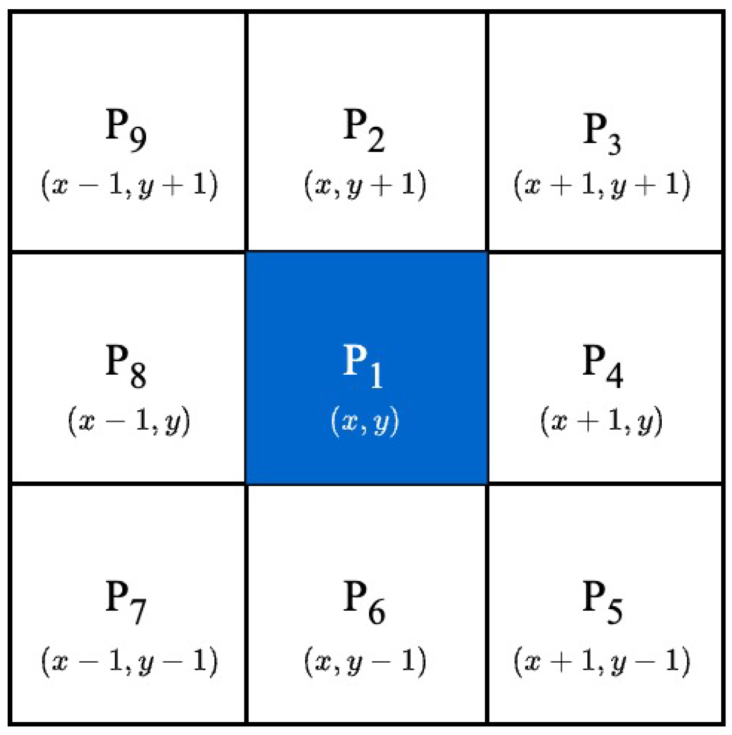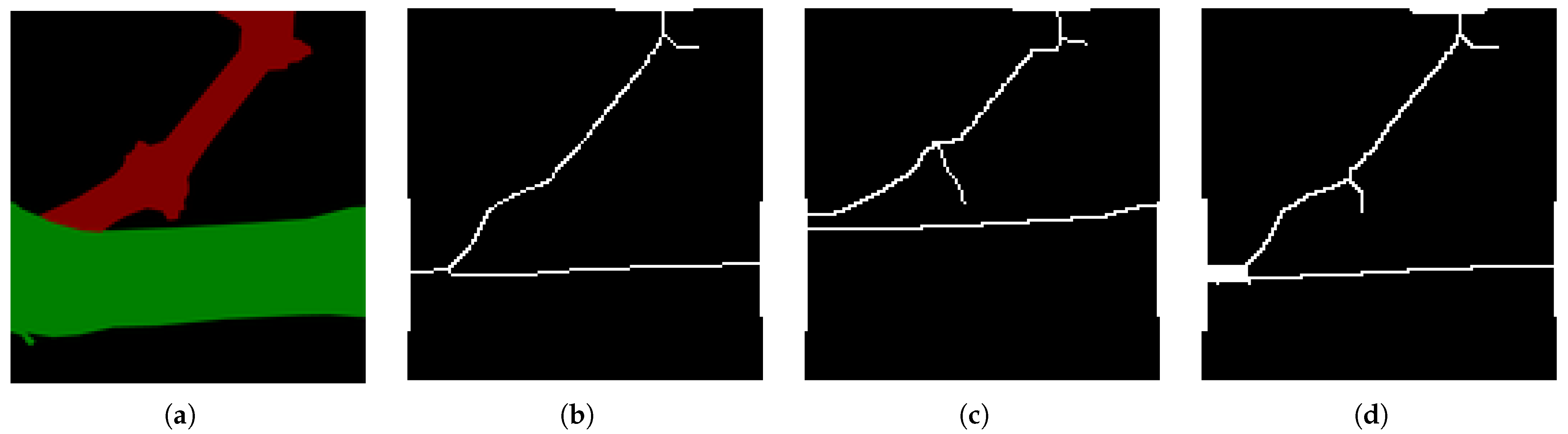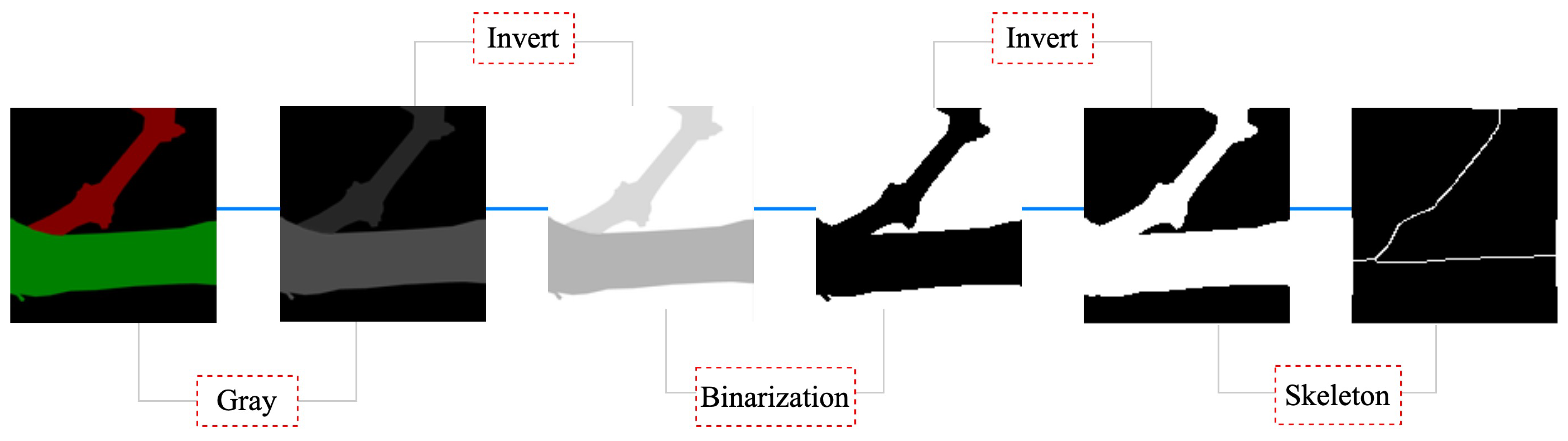In addition, You [27] and others used the topology and geometric priors of an upright fruit branch (UFO) tree to generate such labeled skeletons in order to reconstruct a three-dimensional model of a cherry tree. A skeleton thinning algorithm was applied to the point cloud and the number of manually labeled skeleton segments was used as an accuracy measure, achieving an accuracy of 70%. For the growth characteristics of winter wine grape branches and planting characteristics, i.e., simple tree shape, no foliage shade, etc., you can refer to the above literature for the treatment of branch thinning.

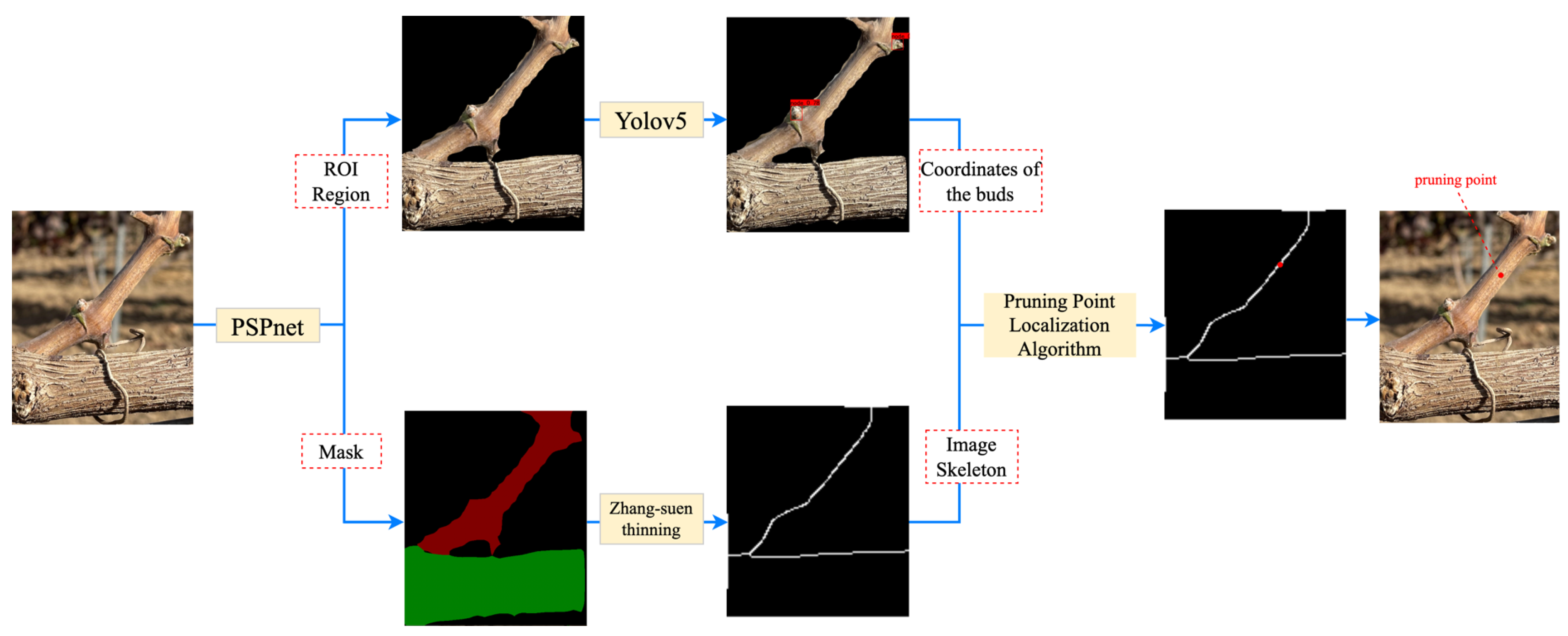
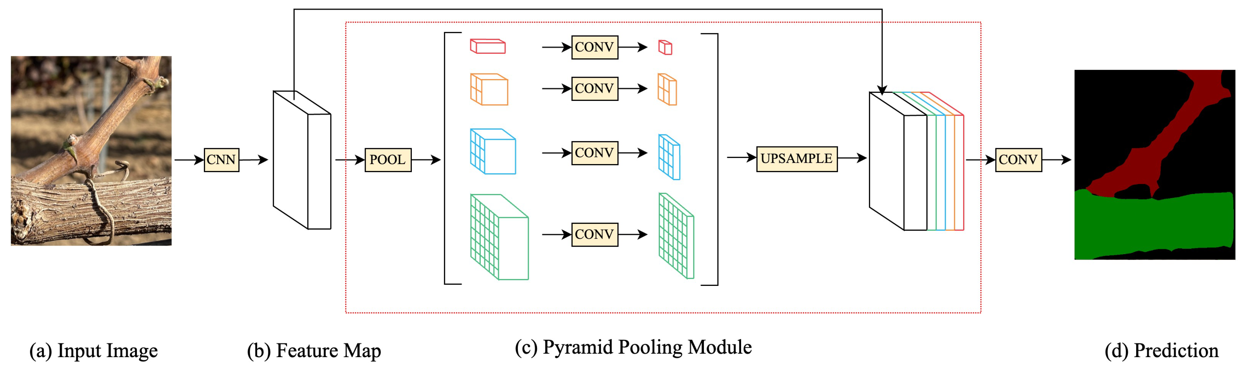
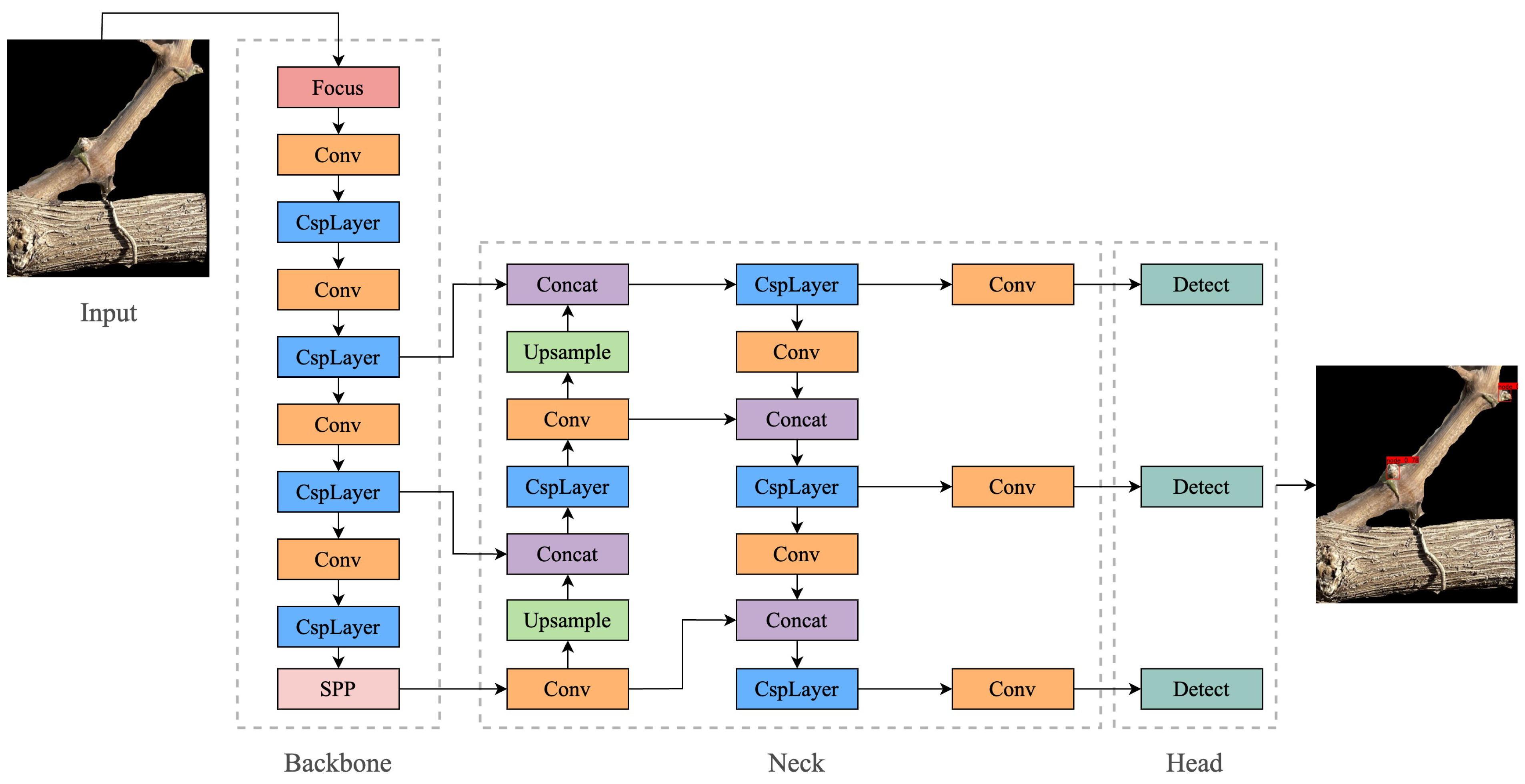
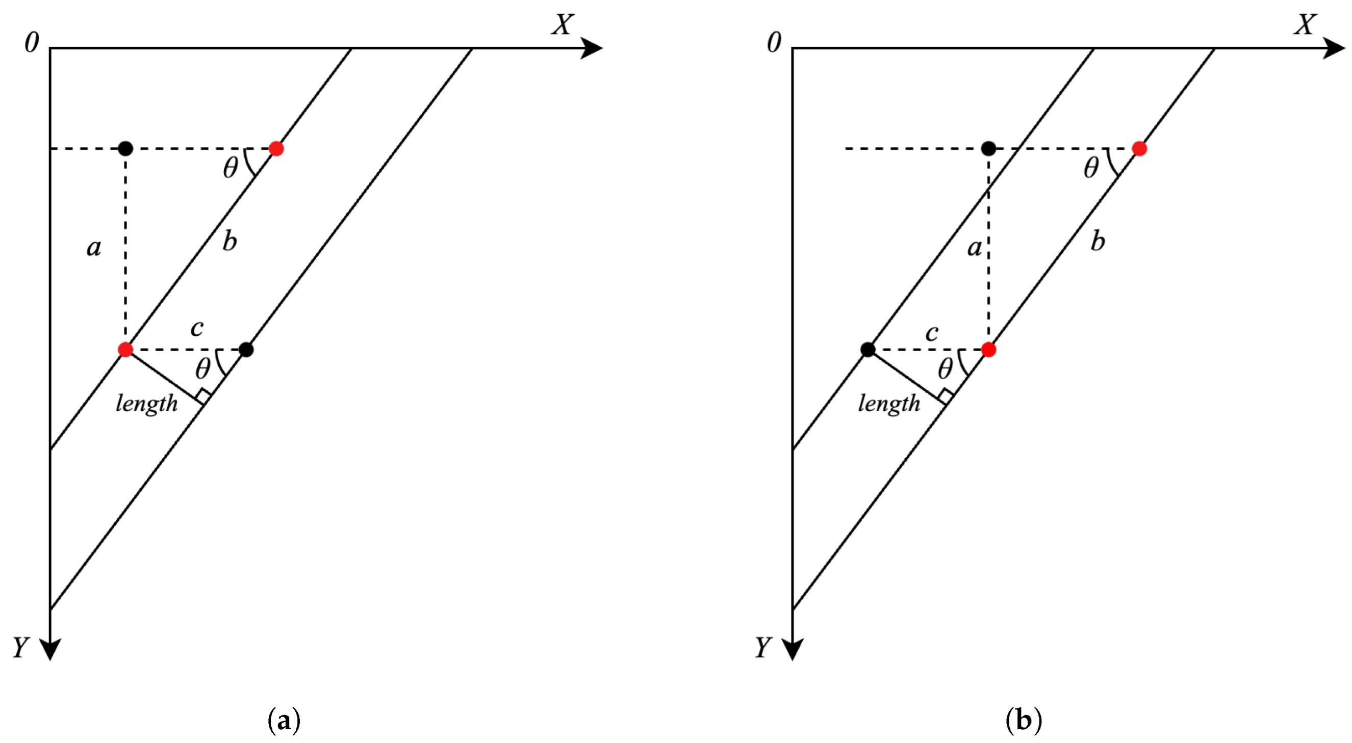
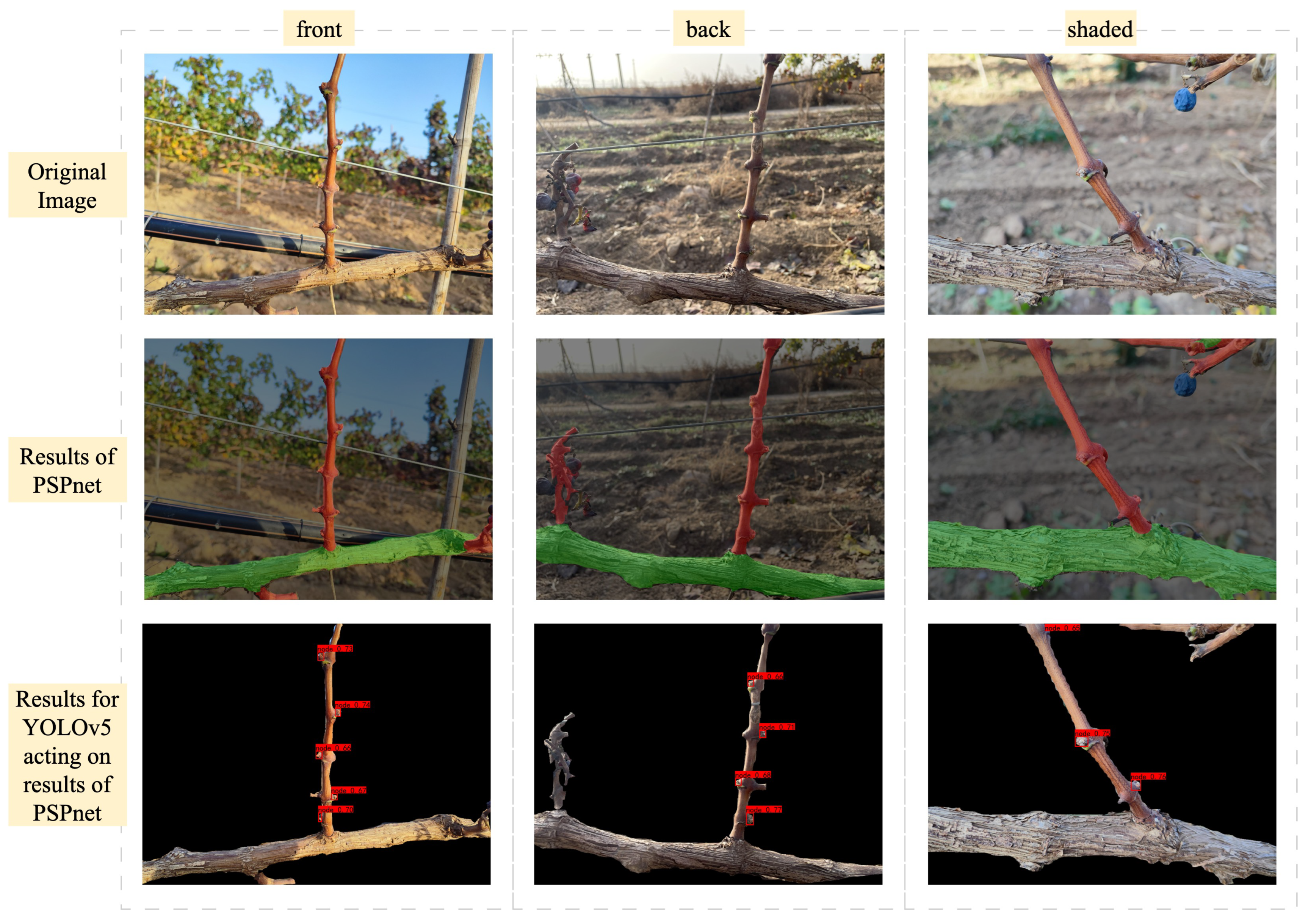
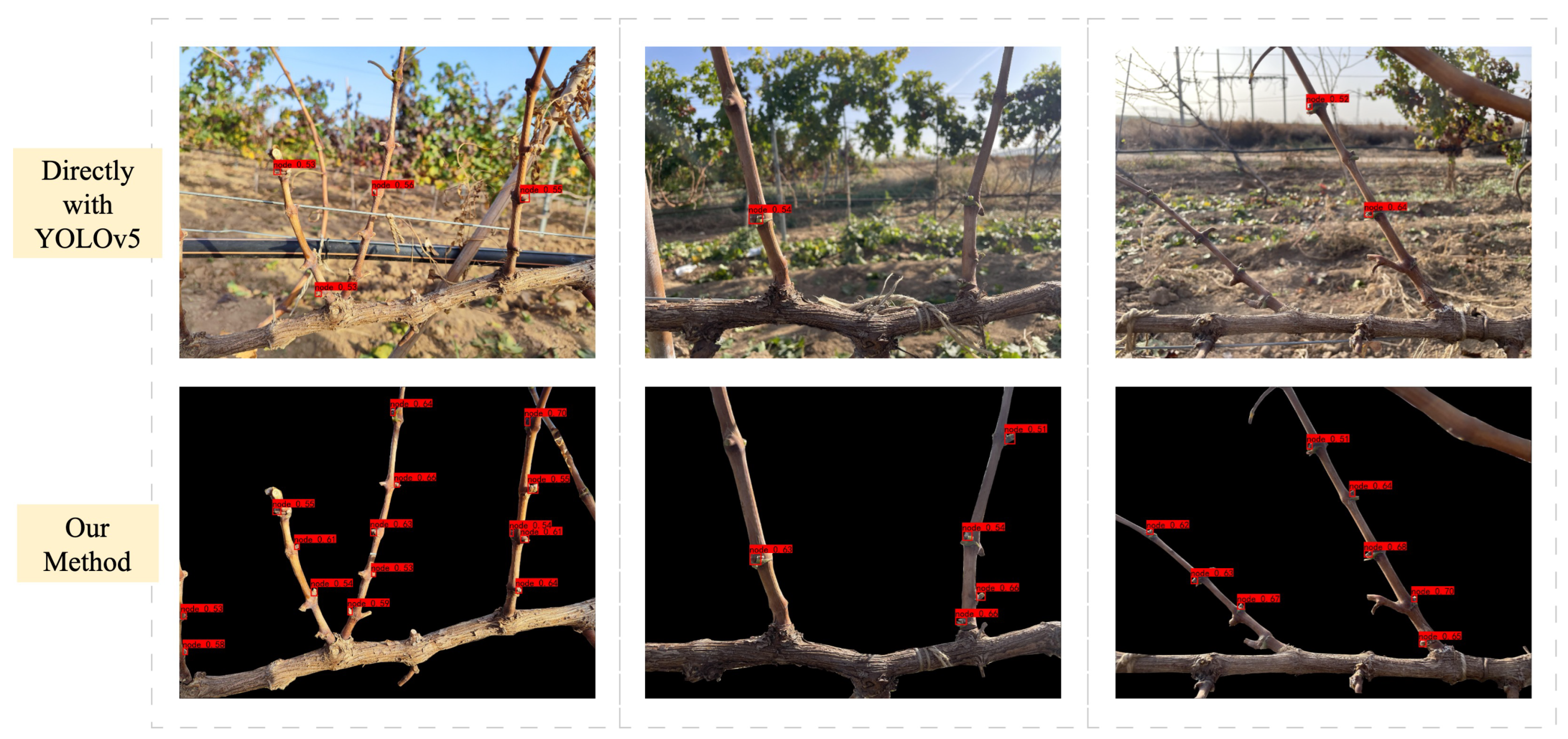
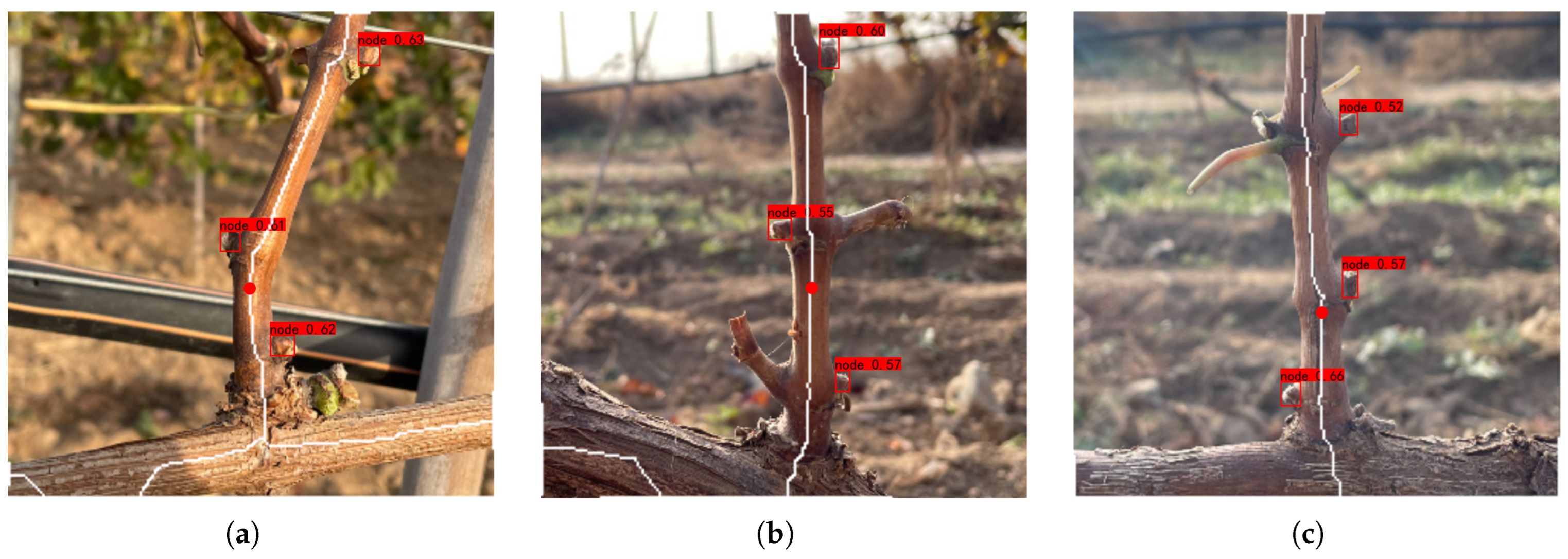
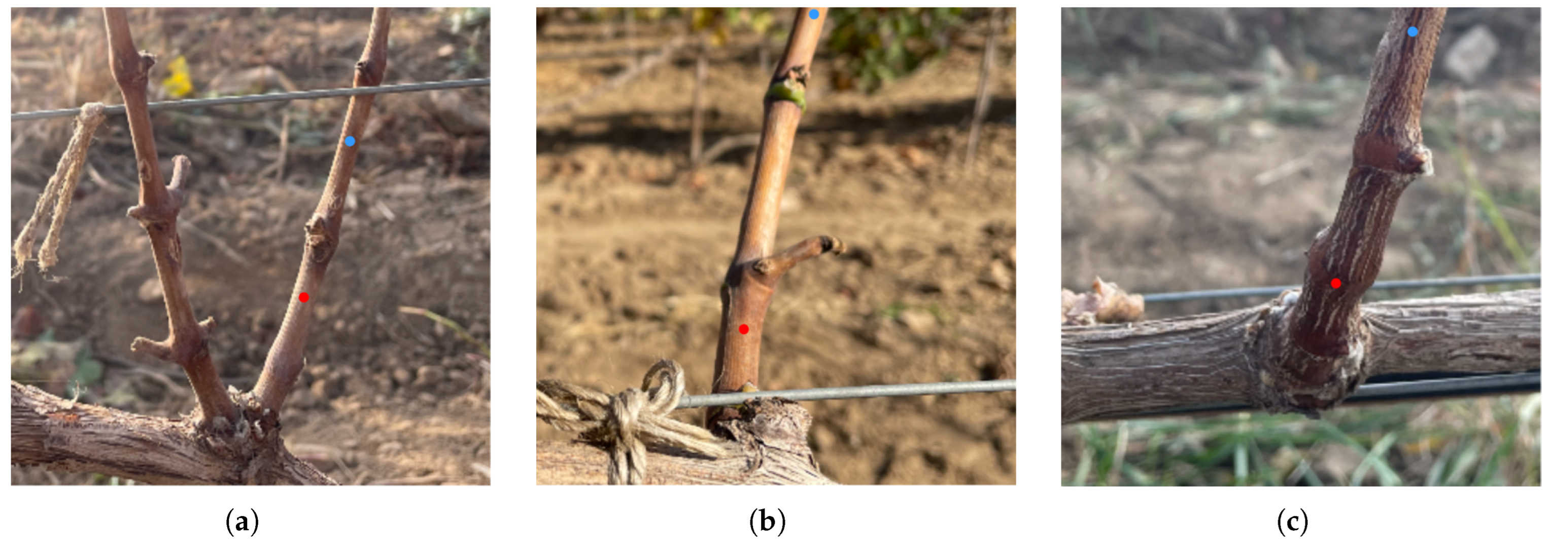
According to the pruning rule, the buds of the object to be recognized in this experiment have the characteristics of small size and similar color to the branches; if we directly use the semantic segmentation algorithm or the target-detection algorithm to detect the branches and the buds at the same time, the features of the buds are not obvious and the branches, which are the main structure, are more easily captured by the model, so the following research objectives are adopted in this experiment: the specific research objectives of this paper are (1) to use semantic segmentation algorithms to segment grape branches, the main stem and the background; (2) to use target-detection algorithms on the segmented image to determine the location of the buds on the branches; (3) to carry out skeleton thinning on the segmented branches; and (4) to determine the location of the clipping point by combining the pruning rules and depth information.

2. Materials and Methods

2.1. The Process of Obtaining Pruning Points

The process of obtaining pruning points proposed in this study is shown in Figure 1. The process of localizing the pruning points on the grape branches is divided into the following steps. (1) Input the original RGB image into the PSP-net network model, segment the branches and trunks and obtain the ROI image and image mask with the background removed. (2) The ROI image is input into the YOLOv5 model to identify the buds and determine the center coordinate points of the buds. (3) The image mask is input into the Zhang–Suen thinning algorithm to extract the centerline and obtain the skeleton of the image. (4) Whether the bud is a key point is determined, that is, the second bud described in Section 2.3, the depth information of the image is combined, the location of the pruning point on the skeleton line is determined and the coordinates are made to correspond to the pixel coordinates in the original image.

2.2. Experiment Location

The experiment site is located in Xixinbao Village, Tumu Town, Huailai County, Zhangjiakou City, Hebei Province, China. The wine grape plantation covers an area of about 6500 acres and is divided into six vineyards with different soil conditions, of which five large vineyards are planted with Cabernet Sauvignon wine grapes. The experiment’s object is the Cabernet Sauvignon wine grape, which is a high-end raw material for Great Wall wine in the market. The planting density is 0.8 m × 2.8 m, with a spacing between plants of 0.8 m and a spacing between rows of 2.8 m, as shown in Figure 2.

A single hedge framework and a single trunk and single arm tree shape for planting are used. In actual production, load-bearing steel wires are used to fix annual branches (i.e., fruiting branches). The first load-bearing steel wire is 30–40 cm away from the ground, as shown in Figure 3. Through the 50 sets of data we measured, we can obtain that the average diameter of the main trunk near the first branch is 21.51 cm. The diameter of annual branches is concentrated between 8 and 10 cm and the growth angle of branches is between 30° and 90°. The grape tree is a deciduous tree that needs to be pruned in winter and buried in soil to prevent the negative effects of the cold. The experimental data were collected from 31 October to 1 November.

2.3. Pruning Rules

According to the staff of the grape-growing base, winter pruning in cutting off branches needs to retain the two buds closest to the trunk, and a pruning position from the second bud of 1–2 cm. As shown in Figure 4a, the red oval is the base of the branch, which will sprout the first bud and the red boxes are the second, third and fourth buds in descending order. Figure 4b shows several clipping scenarios, where scenario c is the correct clipping position. In addition, when the distance between bud 2 and bud 3 is small, it is also possible to cut from bud 3, as shown in case b. Case d is the wrong pruning position, where positioning too close to bud 2 will lead to water loss and reduce the germination rate of the second bud. Cases a and e are incorrect pruning positions; case a retains three buds and reduces the quality of the grapes; case e retains one bud and reduces the yield. Cabernet Sauvignon wine grapes are among the varieties that the site supplies to high-end red wines, so it is important to ensure both yield and quality.

2.4. Dataset Acquisition

This experiment uses two different devices to capture data. First, a Realsense d435i depth camera is used to capture depth images and RGB images, obtaining depth information with a pixel size of 1280 × 720. Then, an iPhone 12 is used to capture RGB images with a pixel size of 4032 × 3024, with a shooting distance of 30–80 cm from the main trunk and a shooting height of 30–40 cm, which is basically the same as the first load-bearing steel wire. Capturing images at different angles of light on sunny days, 500 images were obtained with front light, 314 images with back light and 313 images were obtained with shaded light, totaling 1127 samples. Using methods such as brightness adjustment, image translation and image flipping for data augmentation, 2254 training samples were processed. Random selection was conducted based on a ratio of 6:2:2 for the training set, validation set and test set, resulting in 1352 training samples, 451 validation samples and 451 test samples. The test data are also divided into 200, 126 and 125 sheets based on front light, back light and shaded light. This experiment requires the design of two datasets. The first one is used to segment the main trunk and branches. The original image is annotated using LabelMe [28], labeled as Main Cordon and Cane, as shown in Figure 5a. A VOC format dataset [29] is created. The second method is used to detect the position of buds. The RGB values of the colors in the mask generated after annotation of the first dataset are made transparent and then made to overlapped with the original image. The RGB values of the colors in the overlapped image are made transparent, resulting in a new image. The new image is annotated with Labelimg and labeled as node, as shown in Figure 5b, to create a VOC format dataset. The specific information of the two datasets is shown in

Table 1. Number of images in the dataset.

Label	Tool	Object	Train	Val	Test			Format
					Front	Back	Shaded
Cane Cordon	LabelMe	Original	1352	451	200	126	125	VOC
node	Labelimg	processed

.

2.5. Environment Parameters

The computer is running on the Ubuntu 20.04 operating system with a Tesla V100-SXM2-16GB GPU. The deep learning framework is TensorFlow gpu2.2.0 and the Python version is 3.7. The pip package management tool is used to install third-party Python libraries, such as cudnn, numpy, opencv Python, etc., to achieve deep learning, scientific computing and graphic drawing functions. The key libraries used and their corresponding compatible versions are shown in

Table 2. Python library and their versions.

Python	CUDA	Cudnn	Scipy	Numpy	Matplotlib	Opencv-python	Tqdm	Pillow	H5py
3.7	10.1	7.6	1.4.1	1.18.4	3.2.1	4.2.0.34	4.46.1	8.2.0	2.10.0

.

Choose the appropriate batch size based on computer hardware performance. Meanwhile, selecting appropriate weight decay hyperparameters can prevent overfitting or underfitting. After several debugging sessions, the hyperparameter settings for each model training are shown in

Table 3. Hyperparameter settings.

Model	Batch Size	Epoch	Optimizer	Initial Learning Rate	Learning Rate Decay Type	Momentum
U-net	4	100	sgd	$1\times {10}^{-2}$	cos	0.9
deeplabv3+	16
PSP-net	16
YOLOv3	16	300	adam	$1\times {10}^{-3}$	cos	0.937
YOLOv4	16
YOLOv5	8
YOLOv7	4

.

2.6. Semantic Segmentation Algorithm

PSP-Net Network Model

PSP-net has achieved good performance in semantic segmentation tasks and has been widely used in image segmentation, especially in tasks that require fine segmentation of complex scenes.The PSP model proposes a pyramid pooling module that is able to aggregate the contextual information of different regions to improve the ability to obtain global information. The model structure is shown in Figure 6. A deep convolutional neural network, such as ResNet or VGG, is first used to extract features from the input image. The acquired feature layer is divided into grids of different sizes, i.e., subregions of 6 × 6, 3 × 3, 2 × 2 and 1 × 1 sizes and average pooling is performed inside each subregion. The module aggregates contextual information from different regions to improve the ability to acquire global information. The output of the pyramid pooling module is combined with the feature maps extracted from the backbone network through operations such as up-sampling and finally generates pixel-level semantic segmentation predictions.

2.7. Target-Detection Algorithms

YOLOv5 Network Model

The YOLOv5 model, characterized as lightweight, demands fewer computational resources during training and possesses a compact average weight file while maintaining high detection accuracy, making it conducive for deployment on mobile devices. The model’s architecture, depicted in Figure 7, comprises four components: Input, Backbone, Neck and Prediction. Firstly, the Input layer accepts images as input to the model. YOLOv5 adopts the mosaic data enhancement method and adaptive image scaling module for the input images, which can effectively improve the generalization ability and robustness of the model and make the model achieve good detection results on complex backgrounds and targets with different scales. Backbone consists of a series of convolutional and pooling layers, which are designed to capture low-level and high-level features from the input images. The backbone network of YOLOv5 uses CSPDarknet53, which is a modified Darknet53 architecture that utilizes Cross Stage Partial connections to improve the efficiency and performance of the network. The neck employs multiple feature fusion mechanisms to integrate information from multiple spatial scales. With Feature Pyramid Networks (FPNs) and PAN networks to fuse features at different levels and a CSP structure to enhance the feature fusion capability, the model is able to efficiently capture contextual information and spatial relationships between targets, improving its ability to accurately detect and localize objects of interest. Finally, the prediction header consists of a series of convolutional and linear layers for mapping the extracted features into the space of detection bounding boxes and categories. YOLOv5 uses the CIoU loss as a loss function for the bounding box to improve the speed and accuracy of the regression prediction box.

2.8. Thinning Algorithm

In order to find the subsequent determination of the location of the pruning point, it is necessary to obtain the skeleton thinning map of the branch and the main trunk. First, the image is processed; the color image after semantic segmentation is converted into a grayscale image and then it is binarized; the pixel value corresponding to the background region is 0 and the pixel value corresponding to the ROI region is 1. The binarized image is inputted into the thinning algorithm and the two-dimensional skeleton of the branches and the main trunk is extracted. The higher the image resolution, the higher the number of pixels in the image. The higher the number of iterations, the longer the time for each iteration. In actual processing, the thinning time for an image with a resolution of 1070 × 1262 is as long as 10 min, which does not meet the requirements of real-time recognition in this project. Therefore, the resolution of the image needs to be reduced before proceeding with the thinning algorithm. This experiment evaluates three skeleton thinning algorithms, the Zhang–Suen thinning algorithm [30], the Hilditch thinning algorithm [31] and the Stentiford thinning algorithm [32], and in accordance with the results the Zhang–Suen thinning algorithm is chosen as the thinning algorithm used in this paper.

Zhang–Suen Thinning Algorithm

The Zhang–Suen thinning algorithm refines an image by iteratively deleting pixel points in the image. The pixel point is judged to be removed or not based on the pixel value of its neighborhood. The eight neighbors of a pixel point (x,y) are shown in Figure 8.

The algorithm is divided into two main steps: for the foreground pixel (x,y). (a) if the four Equations (1)–(4) are satisfied, its pixel value is set to 0 and marked for deletion.

$$2⩽B\left(P_1\right)⩽6$$

(1)

$$A\left(P_1\right)=1$$

(2)

$$P_2\times P_4\times P_6=0$$

(3)

$$P_4\times P_6\times P_8=0$$

(4)

where $B\left(P_1\right)$ indicates the number of foreground pixels in the eight pixels adjacent to P1. $A\left(P_1\right)$ denotes the cumulative number of occurrences of 0 to 1 in pixels from P2 to P9 to P2, where 0 denotes the background and 1 denotes the foreground.

(b) If the four Equations (1), (2), (5), (6) are satisfied, the pixel value is set to 0 and marked for deletion.

$$P_2\times P_4\times P_8=0$$

(5)

$$P_2\times P_6\times P_8=0$$

(6)

Repeat steps (a) and (b) until the image no longer changes.

In order to meet the experimental requirements of this paper, the Zhang–Suen refinement algorithm is modified by changing Equations (1) to (7) and it can be seen in RESULT3.1 that the modified Zhang–Suen refinement algorithm has fewer branches and is more suitable for determining the location of pruning points.

$$1⩽B\left(P_1\right)⩽6$$

(7)

2.9. Pruning Point Localization Algorithm

2.9.1. The Basic Principle of Pruning Point Localization Algorithm

The coordinates of the buds obtained via the target-detection algorithm are processed. (1) First, it is determined whether the pixel coordinates of the buds can be connected by the mask map obtained via the semantic segmentation algorithm, i.e., whether there is a path between the pixel coordinates with a pixel value not 0 on the mask map and if there is, the buds are buds on the same branch are determined and are saved in the set of coordinates corresponding to the branch. (2) For the comparison of the coordinates of the buds on the same branch, the coordinate with the largest vertical coordinate is selected as the key point for determining the clipping point. (3) The longitudinal coordinates of the pixel coordinates of the key point are decreased, the horizontal coordinates from left to right are traversed within a certain range and when the pixel value of the skeleton refinement image at this coordinate is not 0, this coordinate position is marked as the pruning point and its 3D coordinates are determined.

2.9.2. Pixel Coordinates to Spatial Coordinates

The process of using depth information to obtain spatial coordinates and spatial distance of pixel coordinates is: (1) Pixel coordinates (a, b) are converted into camera coordinates (x, y, z):

$$\begin{array}{cc}\hfill \left[\begin{array}{c}x\\ y\\ z\end{array}\right]& =K^{-1}\left[\begin{array}{c}a\\ b\\ 1\end{array}\right]·Z_d,K=\left[\begin{array}{ccc}{f}_x& 0& c_x\\ 0& f_y& c_y\\ 0& 0& 1\end{array}\right]\hfill \end{array}$$

(8)

where K is the internal reference matrix of the depth camera, $f_x$, $f_y$ is the camera focal length, $(c_x,c_y)$ is the principal point location and $Z_d$ is the depth information.

(2) Camera coordinates (x, y, z) are converted into world coordinates (X, Y, Z)

$$\begin{array}{cc}\hfill \left[\begin{array}{c}X\\ Y\\ Z\end{array}\right]& =E\left[\begin{array}{c}x\\ y\\ z\\ 1\end{array}\right],E=\left[\begin{array}{cc}R& t\\ 0& 1\end{array}\right]\hfill \end{array}$$

(9)

where E is the depth camera’s external reference matrix, R is the rotation matrix and t is the translation vector.

(3) The actual distance d between two points is calculated using the Euclidean distance formula:

$$\begin{array}{cc}\hfill d& =\sqrt{{(X_2-X_1)}^2+{(Y_2-Y_1)}^2+{(Z_2-Z_1)}^2}\hfill \end{array}$$

(10)

The unit is mm, which corresponds to the unit of depth information.

2.9.3. Pruning Point Positioning

The coordinates of the buds obtained via the target-detection algorithm are processed. (1) Firstly, it is determined whether the pixel coordinates of the buds can be connected by the mask map obtained via the semantic segmentation algorithm and the set of coordinates of the buds on the same branch are determined. (2) For the comparison of the coordinates of buds on the same branch, the coordinate with the largest vertical coordinate is selected as the key point for determining the pruning point. (3) We decrease the vertical coordinate of the pixel coordinate of the key point by $\alpha$, traverse the horizontal coordinate from left to right within a certain range and when the pixel value of the skeleton thinning image at this coordinate is not 0, we mark this coordinate position as the pruning point and determine its 3D coordinates.

As shown in Figure 9, the key parameter $\alpha$ is calculated as follows: (1) We traverse the coordinates of the key point on the mask map obtained via semantic segmentation from left to right in a certain range to obtain a pixel length $\gamma$, which is combined with the depth information in the depth image to obtain the actual length c. (2) From the information of the field measurements, it can be known the the value of the length, i.e., the branch diameter, is concentrated between 8 and 10 mm. (3) The value of b is then the pruning length, i.e., 10–20 mm. (4) Formula (11) is introduced according to Formula (12). (5) According to the growth characteristics of grapevine branches, a and c can be regarded as a plane and then the value of alpha can be determined via Formula (13).

$$sin\theta =\frac{a}{b}=\frac{length}{c}$$

(11)

$$a=\frac{b\ast length}{c}$$

(12)

$$\frac{a}{\alpha }=\frac{c}{\gamma }$$

(13)

3. Results

3.1. Results of Semantic Segmentation

3.1.1. Evaluation Indicators

The metrics used in this paper to evaluate the segmentation performance of the semantic segmentation model are mIoU, mPA and Accuracy. where Accuracy is used to evaluate the overall segmentation accuracy of the image, mPA is the average pixel accuracy of the semantic segmentation and mIoU is used to evaluate the average segmentation accuracy across all categories. The formula is as follows:

$$mIoU=\frac{{\displaystyle \sum _1^{k}IoU}}{k}$$

(14)

$$mPA=\frac{{\displaystyle \sum _1^{k}Recall}}{k}$$

(15)

$$Accuracy=\frac{TP+TN}{TP+TN+FP+FN}$$

(16)

3.1.2. Comparison of Results from Different Semantic Segmentation Models

In order to better segment the branches and trunks, we chose three semantic segmentation models PSP-net, U-Net and DeepLab v3+ [33] to test the same dataset. The evaluation indexes of each algorithm are obtained as shown in

Table 4. Hyperparameter settings.

Model	mIoU (%)	mPA (%)	Accuracy (%)	FPS (Frame)
U-net	83.67	91.27	97.26	101.74
deeplabv3+	81.78	87.69	96.23	126.35
PSP-net	83.73	90.32	96.77	152.72

and the data are compared and analyzed to select the most suitable segmentation model for this experiment.

U-net shows high mPA and Accuracy for semantic segmentation, but in actual training, U-net consumes the most computational resources and achieves the longest training time, high computational complexity and slower processing of images. PSP-net achieved the highest mIoU of 83.73%, while PSP-net achieved the highest FPS value of 152.72; PSP-net achieved higher mIoU than the deeplabv3+ network in all the metrics. Considering the segmentation performance and segmentation speed of the model, this paper chooses PSP-net as the semantic segmentation model for grape branch and main vine ROI images. The results of this algorithm acting on different lighting conditions are shown in Figure 10.

3.2. Results of Target Detection

3.2.1. Evaluation Indicators

The main metrics used to assess the performance of an object-detection model are Recall, Precision, $F_1$ score and mAP. The higher the AP, the higher the Precision of the model. The higher the Recall, the lower the miss rate of the model. In general, the higher the $F_1$ score, the more stable and robust the model is. The Recall, Precision and $F_1$ formulas are as follows:

$$Recall=\frac{TP}{TP+FN}$$

(17)

$$Precision=\frac{TP}{TP+FP}$$

(18)

$$F_1=2·\frac{Precision·Recall}{Precision+Recall}$$

(19)

3.2.2. Comparison of Results from Different Object-Detection Models

We selected four target-detection models, YOLOv3, YOLOv4, YOLOv5 and YOLOv7, to test the same dataset. As shown in

Table 5. Hyperparameter settings.

Model	mAP (%)	Recall (%)	Precision (%)	F1	FPS (Frame)
YOLOv3	75.06	74.81	82.22	0.78	20.93
YOLOv4	72.38	51.32	80.99	0.63	27.32
YOLOv5	81.06	77.78	83.05	0.80	32.78
YOLOv7	80.73	64.02	82.31	0.72	37.98

, the evaluation metrics of each algorithm were obtained and the data were compared and analyzed to select the most suitable segmentation model for this experiment.

From the detection results of different detection models for the region near the pruning point in the table, YOLOv7 exhibits the highest FPS value of 37.98, indicating a high detection speed. However, it demonstrates a lower F₁ score. Conversely, YOLOv5 showcases the highest mAP value of 81.06% and an F₁ value of 0.80, suggesting superior detection performance for the present study. Accurate detection of the area near the pruning point is essential for identifying the pruning point of grapevine branches. Therefore, YOLOv5 was selected as the target-detection model for detecting buds. The results of this algorithm under different lighting conditions are illustrated in Figure 10.

As shown in Figure 11, compared to directly acting on the original image to identify buds using a target-detection method, our theory significantly improves the ability to recognize the buds, providing a better basis for determining the location of the pruning point later.

3.3. Results of the Thinning Algorithm

3.3.1. Evaluation Indicators

We use the following metrics to evaluate the refinement algorithm.

(a) Average time $\overline{X}$ used to evaluate the running speed of the algorithm.

$$\begin{array}{cc}\hfill \overline{X}& =\frac{t}{N}\hfill \end{array}$$

(20)

where t is the total time the program runs and N is the total number of images processed via the algorithm.

(b) Average refinement rate $\overline{R}$: the refinement rate R is used to evaluate how well the key features of the skeleton are preserved.

$$\begin{array}{cc}\hfill R& =\frac{\mathrm{fgps}-\mathrm{fgpst}}{\mathrm{fgps}}\times 100\hfill \end{array}$$

(21)

$$\begin{array}{cc}\hfill \overline{R}& =\frac{{\sum }_{i=1}^N{R}_i}{N}\hfill \end{array}$$

(22)

where fgps is the number of foreground pixels in the original image before refinement, i.e., the number of pixels with pixel value 1. fgpst is the number of foreground pixels in the image after refinement.

(c) Average sensitivity $\overline{S}$: the sensitivity S is used to evaluate the ability of the refinement algorithm to retain fine structures.

$$\begin{array}{cc}\hfill S& =1-\frac{k}{\mathrm{fgps}}\hfill \end{array}$$

(23)

$$\begin{array}{cc}\hfill \overline{S}& =\frac{{\sum }_{i=1}^N{S}_i}{N}\hfill \end{array}$$

(24)

where k is the number of times the pixel value is indicated to change from 0 to 1.

(d) Average degree of variation $\overline{\Delta T}$. The degree of change $\Delta$T is used for the degree of change in the refinement of the image. The refinement degree T is then used to measure the degree of refinement of the skeleton.

$$\begin{array}{cc}\hfill \Delta T& =1-\frac{T_1}{T_0}\hfill \end{array}$$

(25)

$$\begin{array}{cc}\hfill \overline{\Delta T}& =\frac{{\sum }_{i=1}^N\Delta T_i}{N}\hfill \end{array}$$

(26)

where $T_0$ is the refinement of the original image and $T_1$ is the refinement processed via the refinement algorithm.

3.3.2. Comparison of Results from Different Thinning Algorithms

We chose three refinement algorithms, Zhang–Suen thinning algorithm, Hilditch thinning algorithm and Stentiford thinning algorithm, to test the same dataset and the evaluation metrics obtained are shown in

Table 6. Thinning algorithmic evaluation indicators.

Method	$\overline{\mathit{X}}$ (s)	$\overline{\mathit{R}}$	$\overline{\mathit{S}}$	$\overline{\mathbf{\Delta }\mathit{T}}$
Zhang–Suen	1.29	95.44%	90.87%	99.62%
Hilditch	3.01	94.84%	89.75%	99.51%
Stentiford	1.37	93.51%	89.29	98.15%

.

From the data in Table 6, we can see that the Hilditch algorithm has the longest average running time of 3.01 s and the Zhang–Suen algorithm has the shortest average running time of 1.29 s. the Zhang–Suen algorithm has the highest average thinning rate of 95.44%, which means that the number of foreground pixels after thinning is the lowest. The Zhang–Suen algorithm has the highest average sensitivity of 90.87%. The Zhang–Suen algorithm has the highest degree of change in thinning before and after running the image, which is 99.62%. It can be concluded from the data in the table that the Zhang–Suen algorithm is the best in each evaluation index.

It can be seen through the result graphs of the three thinning algorithms in Figure 12 that the Zhang–Suen thinning algorithm performs the best, the Hilditch algorithm’s thinning results are not in the center of the image but at the edge position and the Stentiford algorithm’s thinning at the intersection of the objects is lower. However, for this paper, in the pruning point location, the requirement of branches and trunk of the thinning map cannot have redundant small branches; otherwise, interference in judging the location of pruning point occurs easily, so in this paper the Zhang–Suen thinning algorithm was modified, as in Formula (7), to obtain the total thinning process as shown in Figure 13.

3.4. Positioning of Pruning Points

As can be seen in Figure 14, the algorithm in this paper can correctly identify the location of the pruning point, but there are still some cases where it is difficult to identify the correct location of the pruning point. For example, the location of the second bud of Figure 15a is at the back of the shooting direction and the bud cannot be observed from the front of the branch. The position of the second bud in Figure 15b is obscured by the fixing wire and the location of the clipping point cannot be recognized either. The bud in Figure 15c is on the side and back of the branch, which leaks out to a smaller area and is also difficult to recognize. In response to Figure 15a,c, we propose that in practical applications, both the left and right sides of the same vine can be photographed to address the effect of the growth position of the buds on the localization of the pruning point.

We recognize 102 pruning points, including the cases mentioned above. The total running time is 157.19 s, with an average time of 1.54 s. And 84 detections are successful in determining the correct location of the pruning points with a success rate of 82.35% as shown in

Table 7. Pruning-point-identification results.

Real Pruning Points	Predicted Pruning Points	Identification Success Rate
102	84	82.35%

.

4. Discussion

4.1. Analysis of Semantic Segmentation Results and Target-Detection Results

After evaluation, PSP-net excels in mIoU metrics, outperforming deeplabv3+ by 1.95%, demonstrating the best image segmentation. Meanwhile, PSP-net also shows excellent performance in terms of frame rate (FPS), with 50.11% and 20.87% improvement compared to U-net and deeplabv3+, respectively. It can be seen that PSP-net has the best segmentation effect and segmentation speed and can process images faster and save computational resources when it is close to the segmentation effect of U-net, which means that PSP-net can be used for real-time monitoring of grapevine branches and can also provide accurate branch shapes for skeleton refinement. Under front back shaded three lighting conditions, PSP-net shows good segmentation effects, which means that the lighting conditions have no obvious effect on the segmentation effect and the algorithm has good generalization ability and can be applied in the grape orchard in complex situations.

After evaluation, we find that the F1 value of YOLOv5 improved by 26.98% compared to YOLOv4; the Recall of YOLOv5 improved by 21.49% compared to YOLOv7; meanwhile, the FPS of YOLOv5 improved by 56.62% compared to YOLOv3. YOLOv5 achieved a good balance between precision and recall and was able to take into account both the accuracy and coverage of the prediction results. YOLOv5 acted on the PSP-net segmented image with good results, was not much affected by the lighting conditions and also had good generalization ability and was able to act on the complex situation of the grape orchard. Due to the small bud targets and the similarity of the color with the background and branches, when the YOLOv5 target-detection algorithm was directly applied to the original image, the recognition rate of buds was low and it was more difficult to locate the pruning point according to the position of the second bud. And after PSP-net segmentation of the image and then recognition, the recognition effect is very good. It still has high accuracy and coverage in the case of being further away from the branch position, thinner branches and smaller buds, and can cope with the situation that the machine needs to be at a larger distance from the plant during actual pruning.

In terms of bud identification, when comparing the method proposed in this paper with that of Díaz et al. [34], we find that in their best results, the Precision reached 1, while the Recall ranged between 0.38 and 0.45. This means that in their method, there are no false detections. In contrast, the method of this paper achieves a Recall rate of 77.78% for bud identification, which is an improvement of at least 72.84 percentage points compared to the method of Díaz et al. Further, when comparing the method of this paper with that of Gentilhomme et al. [35], it can be noticed that they took special measures in data collection, i.e., placing white cloths behind the vines in order to eliminate the actual background interference. The dataset used in this paper, on the other hand, is based entirely on a complex background in a natural environment. The method in this paper can still maintain high recognition performance under the complex background, which is closer to the actual application.

4.2. Analysis of Skeleton Extraction and Positioning of Pruning Point Results

After evaluation, we find that the average processing time $\overline{X}$ of the Zhang–Suen refinement algorithm is reduced by 57.14% compared to the Hilditch refinement algorithm. Meanwhile, the average refinement rate $\overline{R}$ of the Zhang–Suen refinement algorithm is also slightly higher than that of the Stentiford refinement algorithm, specifically 1.93% higher. In this paper, we improve the decision condition of the Zhang–Suen thinning algorithm, which makes the skeleton more focused on the main stem and branches and excludes the influence of other things such as secondary branches or buds growing on branches on the skeleton of the branches, which makes the skeleton of a grapevine obtained after the segmentation more in line with the actual shape and the skeleton line is also in the middle of the branch.

We achieved a detection rate of 82.35% for the location of the pruning point, which is the probability obtained in the case shown in Figure 15. For the specific case of buds growing on the back of a branch, we can improve the detection rate of the pruning point by the detection of the back side of the branch as well. Despite the complexity of the real-world environment, this paper provides an efficient pruning-point-localization method with a high detection rate.

In terms of model running efficiency, we compared the method proposed in this paper with the method used by Williams et al. [36]. According to the results of the comparison, in Williams et al.’s study, the total time required for the system to process 80 scan points to generate a 3D model during the 3D reconstruction phase of the process was between 10 min and 15 min, and subsequently, their vision system processed individual scan points in 15–35 s. In contrast, the model in this paper processes the image and determines the positions of 102 pruning points in only 157.19 s, with each taking 1.54 s. In terms of efficiency, there is a significant difference between them and the method in this paper significantly improves the processing speed.

5. Conclusions

In this study, we innovatively propose a method that combines semantic segmentation and target detection to recognize small objects and ultimately combines them with pruning rules to obtain pruning points. The dataset used in this paper includes grapevine branches under different lighting conditions, which is more in line with the actual working scenario. In this study, we used three semantic segmentation methods and after processing the same dataset with three lighting conditions including front light, back light and shaded light, it was determined that the PSP-net was the most effective, with an mIoU value of 83.73%, an accuracy of 96.77% and an mPA of 90.32%; For bud detection, direct recognition is less efficient due to the smaller target and the higher complexity of the image background, but better results can be obtained after semantic segmentation and then target detection. We compare four target-detection algorithms here, in which YOLOv5 shows better results, with an mAP of up to 81.06%, a Recall of up to 77.78%, Precision reaching 83.05% and F₁ reaching 0.80; combined with the branch pruning rule, that is, pruning 1–2 cm above the second bud, the proposed processing of the bud coordinates accurately obtains the location of the pruning point and the detection rate of pruning point reaches 82.35%. The experiment results show that the method is characterized by a high detection rate and an accurate location of the pruning point. The pruning-point-localization method proposed in this paper for depth images and RGB images has high accuracy, which lays the foundation for our subsequent work, i.e., to obtain the 3D coordinates of the pickup point by combining the image depth information obtained from the depth camera. It also provides a reference for other bud-related pruning rules, such as intelligent pruning for long tip pruning and enhances the ability of intelligent pruning to recognize pruning points under different pruning rules. However, in this paper, some pruning points are still not recognized. In the subsequent research, we can focus on improving the semantic segmentation algorithm and the target-detection algorithm to optimize the segmentation effect of branch edges and improve the recognition accuracy of bud points, so as to improve the accuracy of pruning points. At the same time, extensive test experiments will be conducted on more varieties of grapevines to ensure the generalizability and reliability of the study.

References

1. Yuqiang, L. Grape Winter Management Should not be Ignored. Technical Report. AgroScience News, 5 December 2022. [Google Scholar]
2. Poni, S.; Tombesi, S.; Palliotti, A.; Ughini, V.; Gatti, M. Mechanical winter pruning of grapevine: Physiological bases and applications. Sci. Hortic. 2016, 204, 88–98. [Google Scholar] [CrossRef]
3. Zhang, J.; He, L.; Karkee, M.; Zhang, Q.; Zhang, X.; Gao, Z. Branch detection for apple trees trained in fruiting wall architecture using depth features and Regions-Convolutional Neural Network (R-CNN). Comput. Electron. Agric. 2018, 155, 386–393. [Google Scholar] [CrossRef]
4. Chen, Z.; Ting, D.; Newbury, R.; Chen, C. Semantic segmentation for partially occluded apple trees based on deep learning. Comput. Electron. Agric. 2021, 181, 105952. [Google Scholar] [CrossRef]
5. Ma, B.; Du, J.; Wang, L.; Jiang, H.; Zhou, M. Automatic branch detection of jujube trees based on 3D reconstruction for dormant pruning using the deep learning-based method. Comput. Electron. Agric. 2021, 190, 106484. [Google Scholar] [CrossRef]
6. Li, J.; Tang, Y.; Zou, X.; Lin, G.; Wang, H. Detection of Fruit-Bearing Branches and Localization of Litchi Clusters for Vision-Based Harvesting Robots. IEEE Access 2020, 8, 117746–117758. [Google Scholar] [CrossRef]
7. Yang, C.H.; Xiong, L.Y.; Wang, Z.; Wang, Y.; Shi, G.; Kuremot, T.; Zhao, W.H.; Yang, Y. Integrated detection of citrus fruits and branches using a convolutional neural network. Comput. Electron. Agric. 2020, 174, 105469. [Google Scholar] [CrossRef]
8. Feng, Y.; Ma, W.; Tan, Y.; Yan, H.; Qian, J.; Tian, Z.; Gao, A. Approach of Dynamic Tracking and Counting for Obscured Citrus in Smart Orchard Based on Machine Vision. Appl. Sci. 2024, 14, 1136. [Google Scholar] [CrossRef]
9. Cong, P.; Zhou, J.; Li, S.; Lv, K.; Feng, H. Citrus Tree Crown Segmentation of Orchard Spraying Robot Based on RGB-D Image and Improved Mask R-CNN. Appl. Sci. 2023, 13, 164. [Google Scholar] [CrossRef]
10. Sun, Q.; Chai, X.; Zeng, Z.; Zhou, G.; Sun, T. Multi-level feature fusion for fruit bearing branch keypoint detection. Comput. Electron. Agric. 2021, 191, 106479. [Google Scholar] [CrossRef]
11. Cuevas-Velasquez, H.; Gallego, A.J.; Fisher, R.B. Segmentation and 3D reconstruction of rose plants from stereoscopic images. Comput. Electron. Agric. 2020, 171, 105296. [Google Scholar] [CrossRef]
12. Turgut, K.; Dutagaci, H.; Rousseau, D. RoseSegNet: An attention-based deep learning architecture for organ segmentation of plants. Biosyst. Eng. 2022, 221, 138–153. [Google Scholar] [CrossRef]
13. Koirala, A.; Walsh, K.; Wang, Z.; McCarthy, C. Deep learning for real-time fruit detection and orchard fruit load estimation: Benchmarking of ‘MangoYOLO’. Precis. Agric. 2019, 20, 1107–1135. [Google Scholar] [CrossRef]
14. Redmon, J.; Farhadi, A. Yolov3: An incremental improvement. arXiv 2018, arXiv:1804.02767. [Google Scholar]
15. Redmon, J.; Farhadi, A. YOLO9000: Better, faster, stronger. In Proceedings of the IEEE Conference on Computer Vision and Pattern Recognition, Honolulu, HI, USA, 21–26 July 2017; pp. 7263–7271. [Google Scholar]
16. Roy, A.M.; Bhaduri, J. Real-time growth stage detection model for high degree of occultation using DenseNet-fused YOLOv4. Comput. Electron. Agric. 2022, 193, 106694. [Google Scholar] [CrossRef]
17. Zhou, J.; Zhang, Y.; Wang, J. A dragon fruit picking detection method based on YOLOv7 and PSP-Ellipse. Sensors 2023, 23, 3803. [Google Scholar] [CrossRef]
18. Bochkovskiy, A.; Wang, C.Y.; Liao, H.Y.M. Yolov4: Optimal speed and accuracy of object detection. arXiv 2020, arXiv:2004.10934. [Google Scholar]
19. Li, C.; Li, L.; Jiang, H.; Weng, K.; Geng, Y.; Li, L.; Ke, Z.; Li, Q.; Cheng, M.; Nie, W.; et al. YOLOv6: A single-stage object detection framework for industrial applications. arXiv 2022, arXiv:2209.02976. [Google Scholar]
20. Ge, Z.; Liu, S.; Wang, F.; Li, Z.; Sun, J. Yolox: Exceeding yolo series in 2021. arXiv 2021, arXiv:2107.08430. [Google Scholar]
21. Wang, C.Y.; Bochkovskiy, A.; Liao, H.Y.M. YOLOv7: Trainable bag-of-freebies sets new state-of-the-art for real-time object detectors. In Proceedings of the IEEE/CVF Conference on Computer Vision and Pattern Recognition, Vancouver, BC, Canada, 17–24 June 2023; pp. 7464–7475. [Google Scholar]
22. Chen, Y.; Li, X.; Jia, M.; Li, J.; Hu, T.; Luo, J. Instance Segmentation and Number Counting of Grape Berry Images Based on Deep Learning. Appl. Sci. 2023, 13, 6751. [Google Scholar] [CrossRef]
23. Morellos, A.; Dolaptsis, K.; Tziotzios, G.; Pantazi, X.E.; Kateris, D.; Berruto, R.; Bochtis, D. An IoT Transfer Learning-Based Service for the Health Status Monitoring of Grapevines. Appl. Sci. 2024, 14, 1049. [Google Scholar] [CrossRef]
24. Marani, R.; Milella, A.; Petitti, A.; Reina, G. Deep neural networks for grape bunch segmentation in natural images from a consumer-grade camera. Precis. Agric. 2021, 22, 387–413. [Google Scholar] [CrossRef]
25. Zhong, Z.; Xiong, J.; Zheng, Z.; Liu, B.; Liao, S.; Huo, Z.; Yang, Z. A method for litchi picking points calculation in natural environment based on main fruit bearing branch detection. Comput. Electron. Agric. 2021, 189, 106398. [Google Scholar] [CrossRef]
26. Tong, S.; Yue, Y.; Li, W.; Wang, Y.; Kang, F.; Feng, C. Branch Identification and Junction Points Location for Apple Trees Based on Deep Learning. Remote Sens. 2022, 14, 4495. [Google Scholar] [CrossRef]
27. You, A.; Grimm, C.; Silwal, A.; Davidson, J.R. Semantics-guided skeletonization of upright fruiting offshoot trees for robotic pruning. Comput. Electron. Agric. 2022, 192, 106622. [Google Scholar] [CrossRef]
28. Russell, B.C.; Torralba, A.; Murphy, K.P.; Freeman, W.T. LabelMe: A database and web-based tool for image annotation. Int. J. Comput. Vis. 2008, 77, 157–173. [Google Scholar] [CrossRef]
29. Everingham, M.; Van Gool, L.; Williams, C.K.; Winn, J.; Zisserman, A. The pascal visual object classes (voc) challenge. Int. J. Comput. Vis. 2010, 88, 303–338. [Google Scholar] [CrossRef]
30. Zhang, T.Y.; Suen, C.Y. A fast parallel algorithm for thinning digital patterns. Commun. ACM 1984, 27, 236–239. [Google Scholar] [CrossRef]
31. Hilitch, C.J. Linear Skeletons from Square Cupboards. 1969. Available online: https://philpapers.org/rec/HILLSF (accessed on 18 March 2024).
32. Martin, A.; Tosunoglu, S. Image Processing Techniques for Machine Vision; Citeseer: Miami, FL, USA, 2000; pp. 1–9. [Google Scholar]
33. Chen, L.C.; Zhu, Y.; Papandreou, G.; Schroff, F.; Adam, H. Encoder-decoder with atrous separable convolution for semantic image segmentation. In Proceedings of the European Conference on Computer Vision (ECCV), Munich, Germany, 8–14 September 2018; pp. 801–818. [Google Scholar]
34. Díaz, C.A.; Pérez, D.S.; Miatello, H.; Bromberg, F. Grapevine buds detection and localization in 3D space based on structure from motion and 2D image classification. Comput. Ind. 2018, 99, 303–312. [Google Scholar] [CrossRef]
35. Gentilhomme, T.; Villamizar, M.; Corre, J.; Odobez, J.M. Towards smart pruning: ViNet, a deep-learning approach for grapevine structure estimation. Comput. Electron. Agric. 2023, 207, 107736. [Google Scholar] [CrossRef]
36. Williams, H.; Smith, D.; Shahabi, J.; Gee, T.; Nejati, M.; McGuinness, B.; Black, K.; Tobias, J.; Jangali, R.; Lim, H.; et al. Modelling wine grapevines for autonomous robotic cane pruning. Biosyst. Eng. 2023, 235, 31–49. [Google Scholar] [CrossRef]
Figure 1. The process of obtaining pruning points.
Applsci 14 03327 g001
Figure 2. Experiment site environment.
Applsci 14 03327 g002
Figure 3. Vertical forms of cultivation of grapevine branches.
Applsci 14 03327 g003
Figure 4. (a) Location of buds. (b) Pruning position.
Applsci 14 03327 g004
Figure 5. Two types of datasets: (a) Outline object contours using LabelMe software5.1.1 on the original image. (b) Perform bounding box annotation using Labelimg software1.8.6 on processed images.
Applsci 14 03327 g005
Figure 6. The network structure of PSP-net.
Applsci 14 03327 g006
Figure 7. The network structure of YOLOv5.
Applsci 14 03327 g007
Figure 8. Names of the eight neighbors around the pixel point.
Applsci 14 03327 g008
Figure 9. The branch is inclined to the right with respect to the vertical position. The red dots represent the positions of bud points and pruning points on the branches, while the black dots represent auxiliary points used for drawing guide lines. (a) The case when the bud is on the left side of the branch. (b) The case when the bud is on the right side of the branch.
Applsci 14 03327 g009
Figure 10. Detection results of PSP-net and YOLOv5 models under different light conditions.
Applsci 14 03327 g010
Figure 11. The result of recognizing the buds directly with YOLOv5 and the result of recognizing the buds with our method.
Applsci 14 03327 g011
Figure 12. (a) RGB image. (b) The result image of the Zhang–Suen thinning algorithm. (c) The result image of the Hilditch algorithm. (d) The result image of the Stentiford algorithm.
Applsci 14 03327 g012
Figure 13. The thinning process for an RGB image. First, the image is converted into grayscale; next, inversion processing is performed; then, binarization is applied; subsequently, inversion is performed again; finally, the skeletonization algorithm is applied.
Applsci 14 03327 g013
Figure 14. (ac) represent the correct identification of pruning points under three lighting conditions: front light, back light, and shaded light. Red dots represent pruning positions.
Applsci 14 03327 g014
Figure 15. (a) The bud is directly behind the branch. (b) The bud is obscured by a fixed wire. (c) The bud is to the side and behind the branch. Red dots represent correct pruning positions while blue dots represent incorrect pruning positions.
Applsci 14 03327 g015