
Holoscopic Elemental-Image-Based Disparity Estimation Using Multi-Scale, Multi-Window Semi-Global Block Matching


Abstract
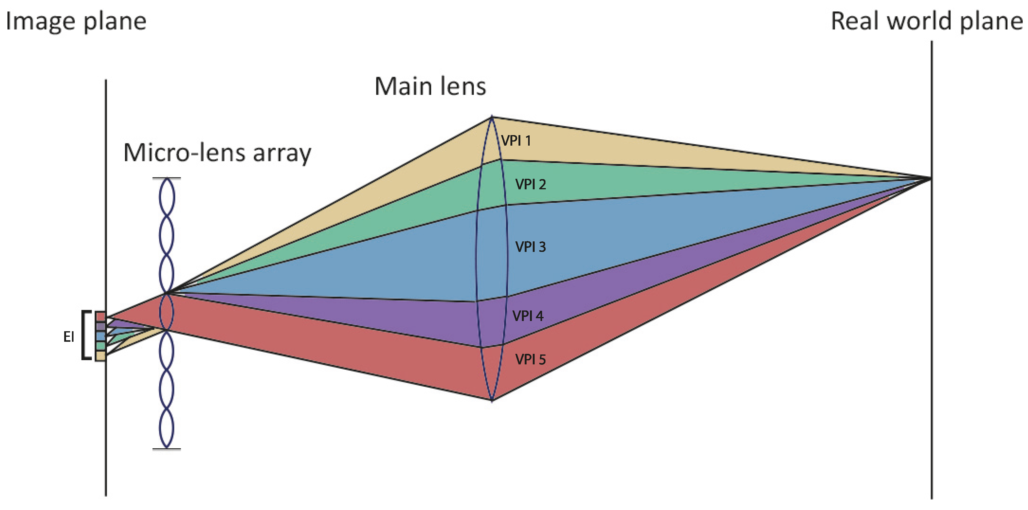
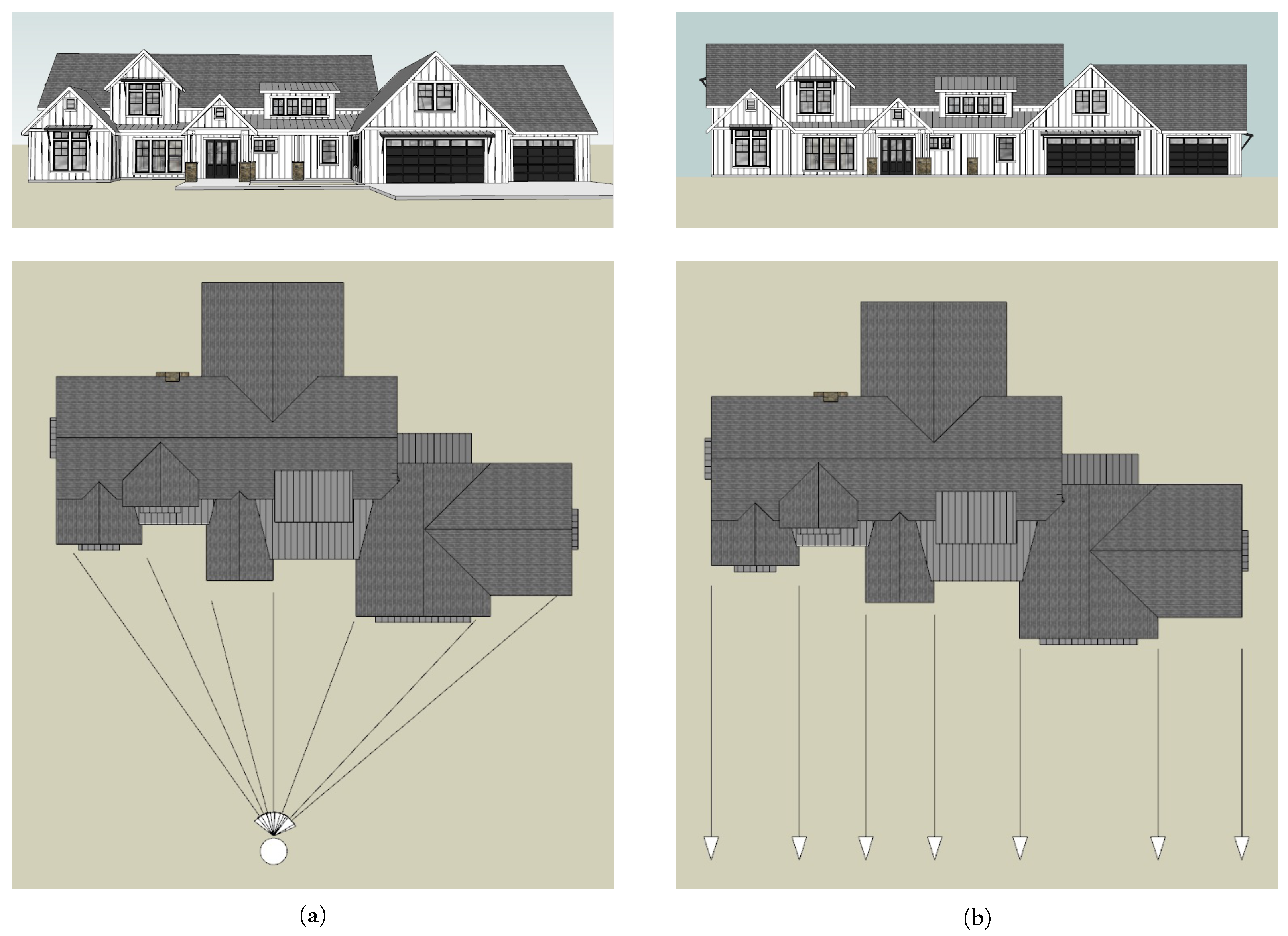
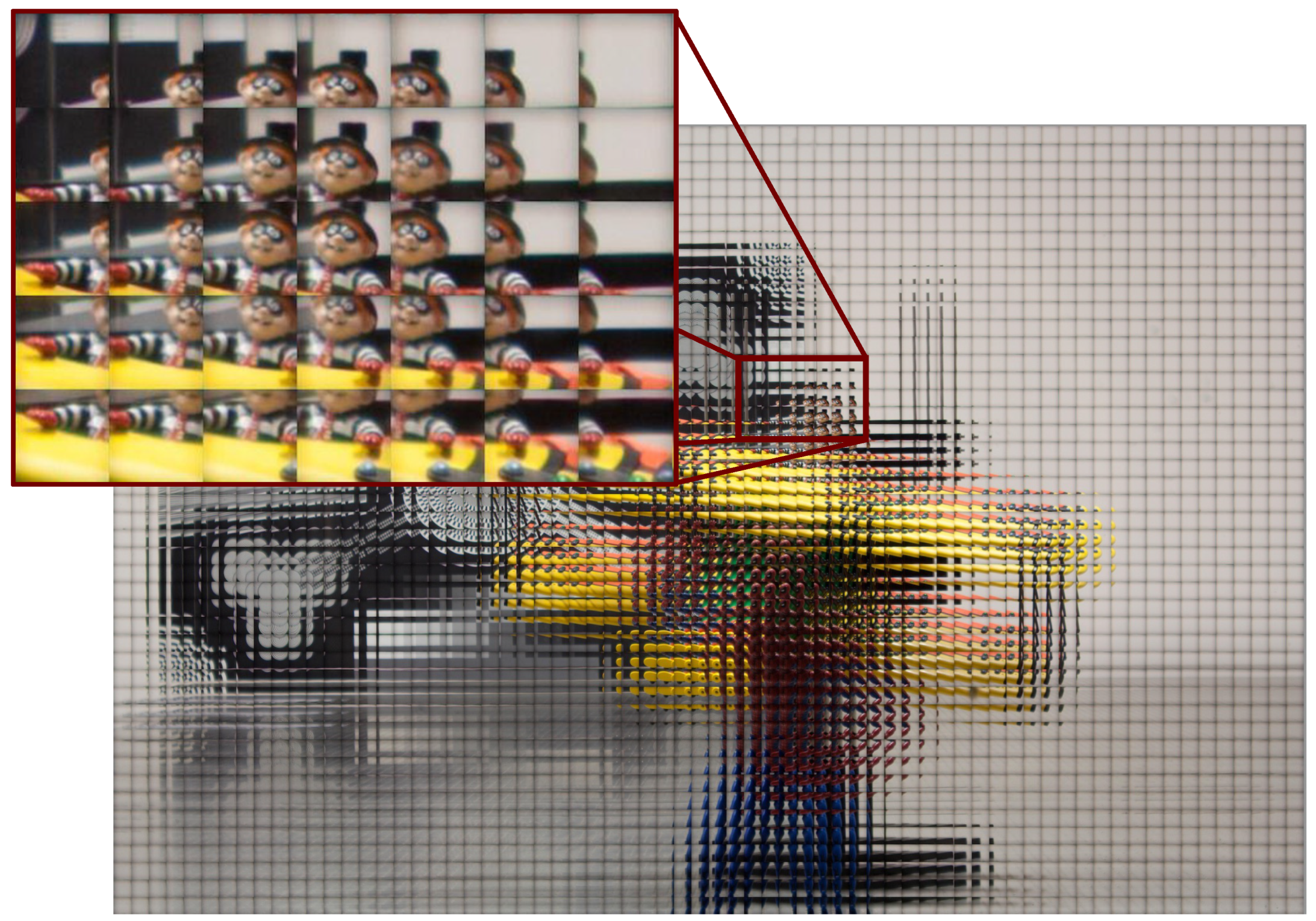
:1. Introduction
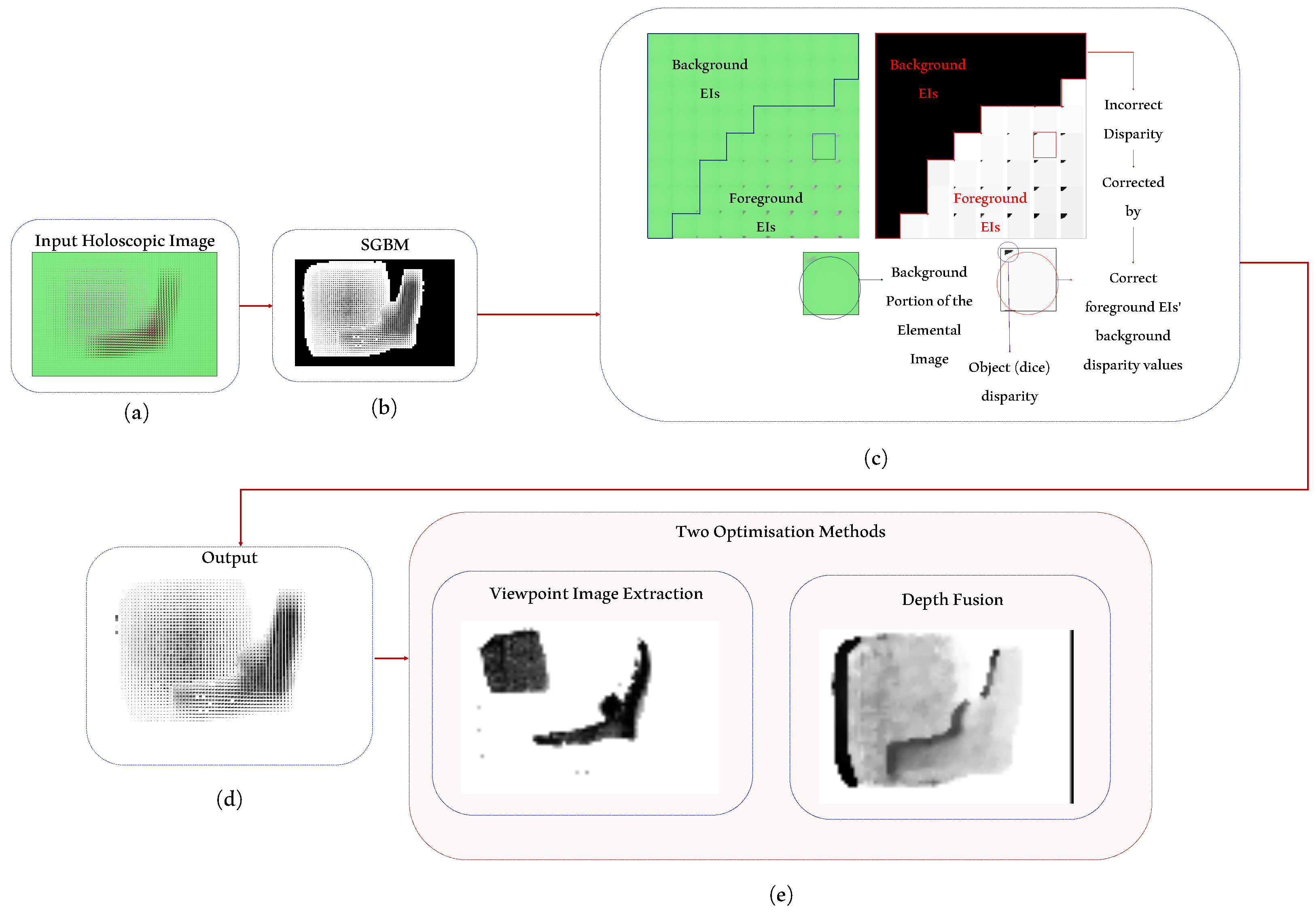
2. Methodology
2.1. Pre-Processing of Elemental Images
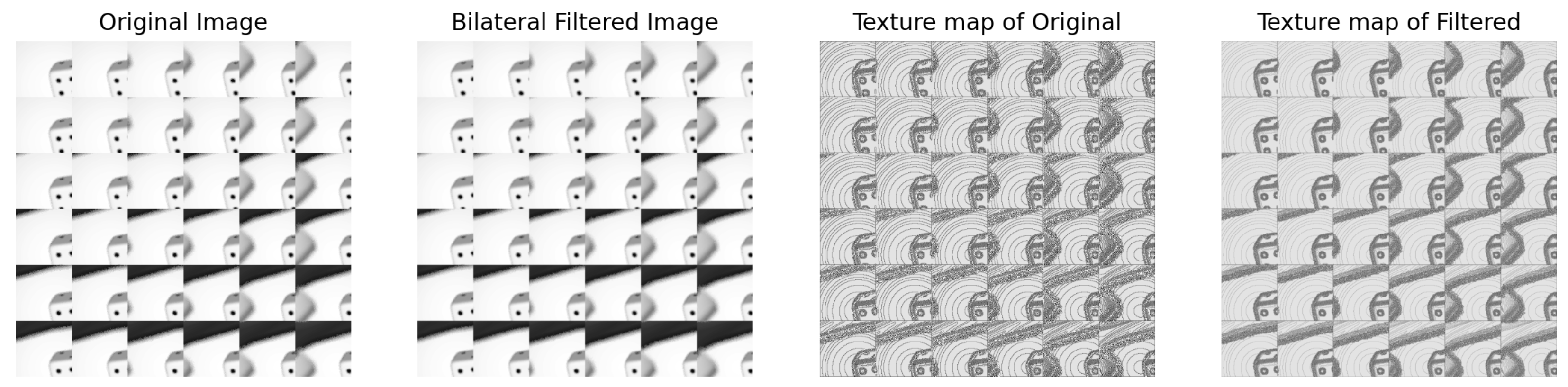
2.1.1. Noise Reduction through Bilateral Filtering
2.1.2. Contrast Enhancement via Histogram Equalisation
2.2. Content-Aware Multi-Resolution Disparity Estimation Using Semi-Global Block Matching
2.2.1. Overview
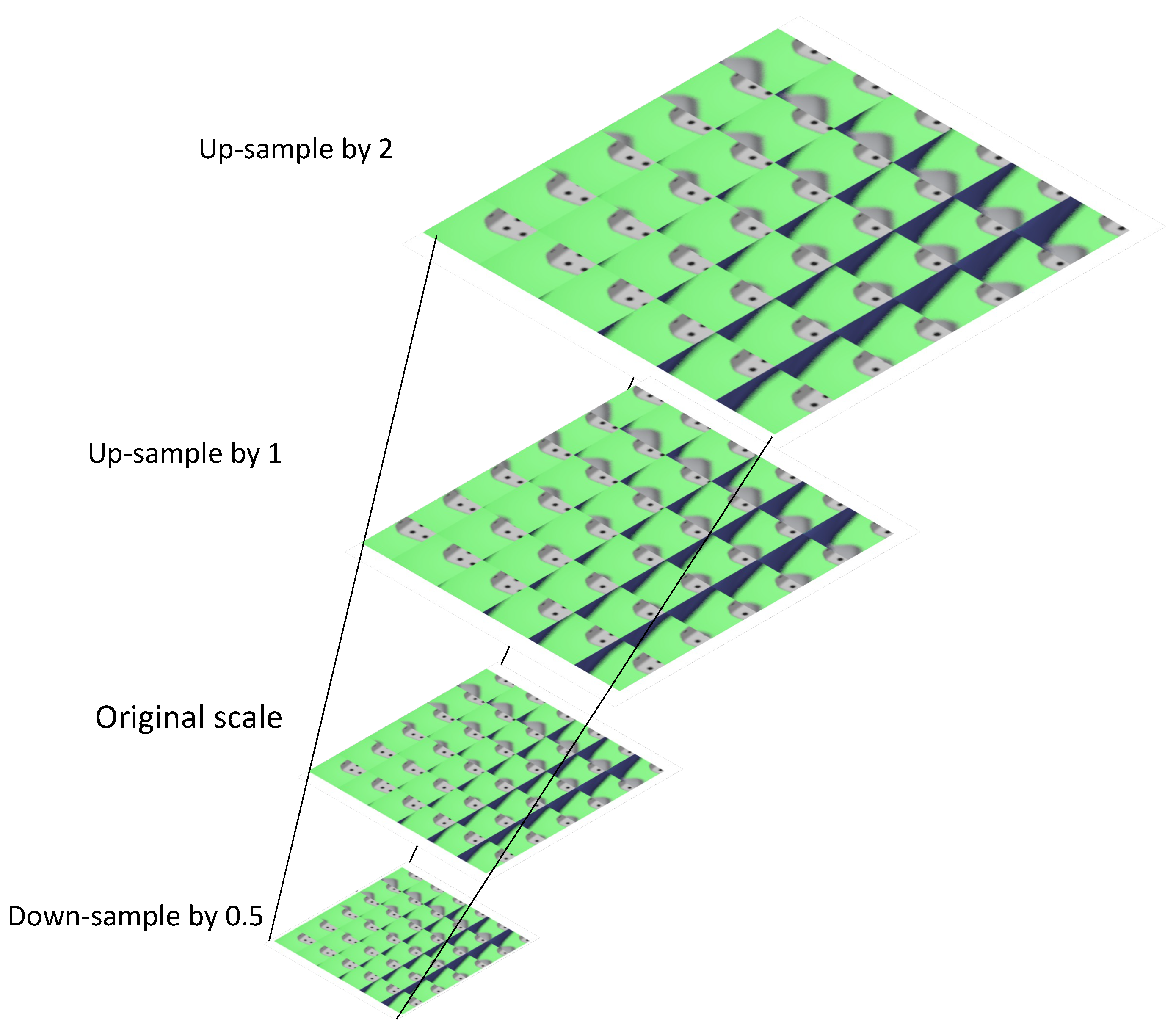
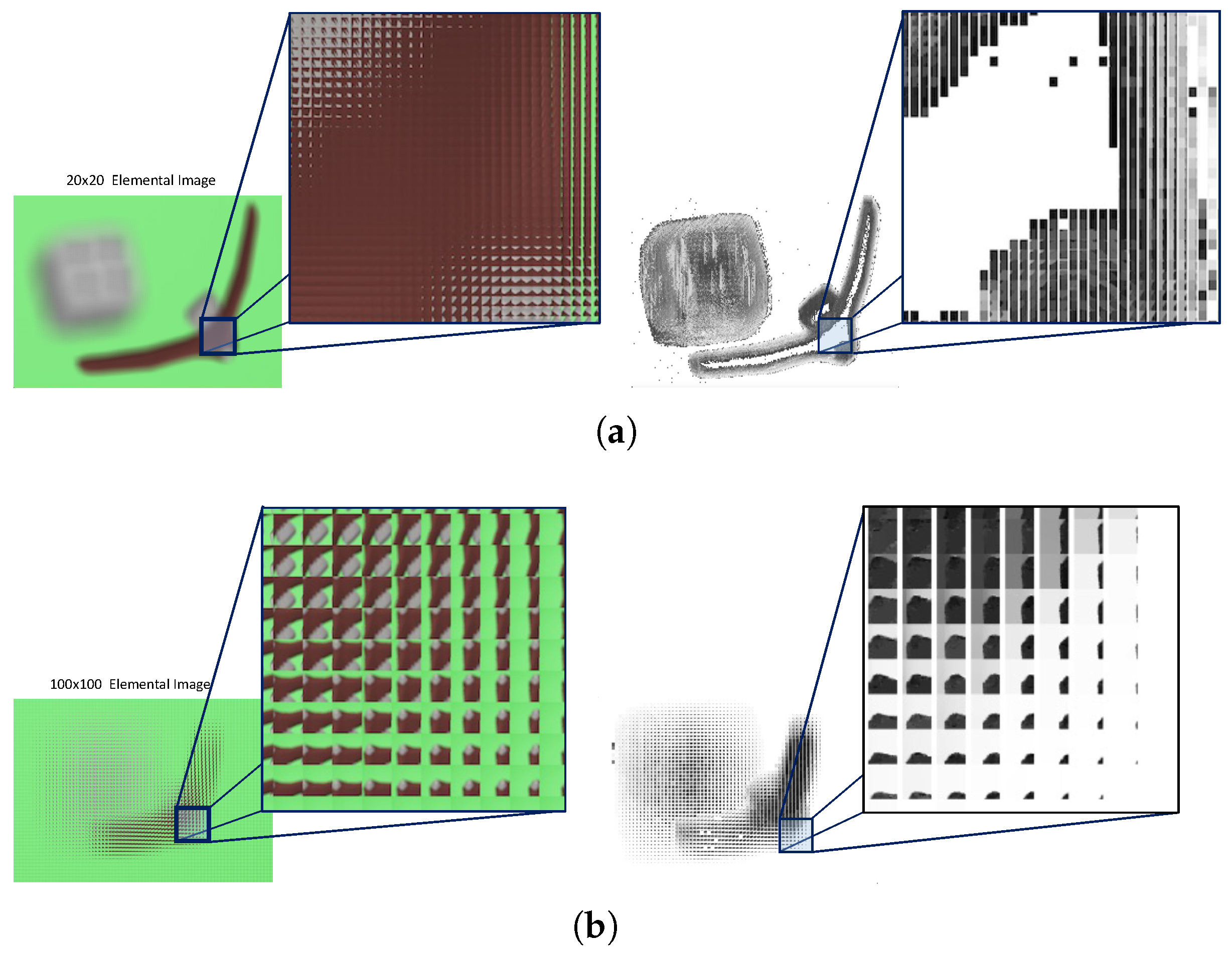
2.2.2. Multi-Resolution Elemental Image Pyramid
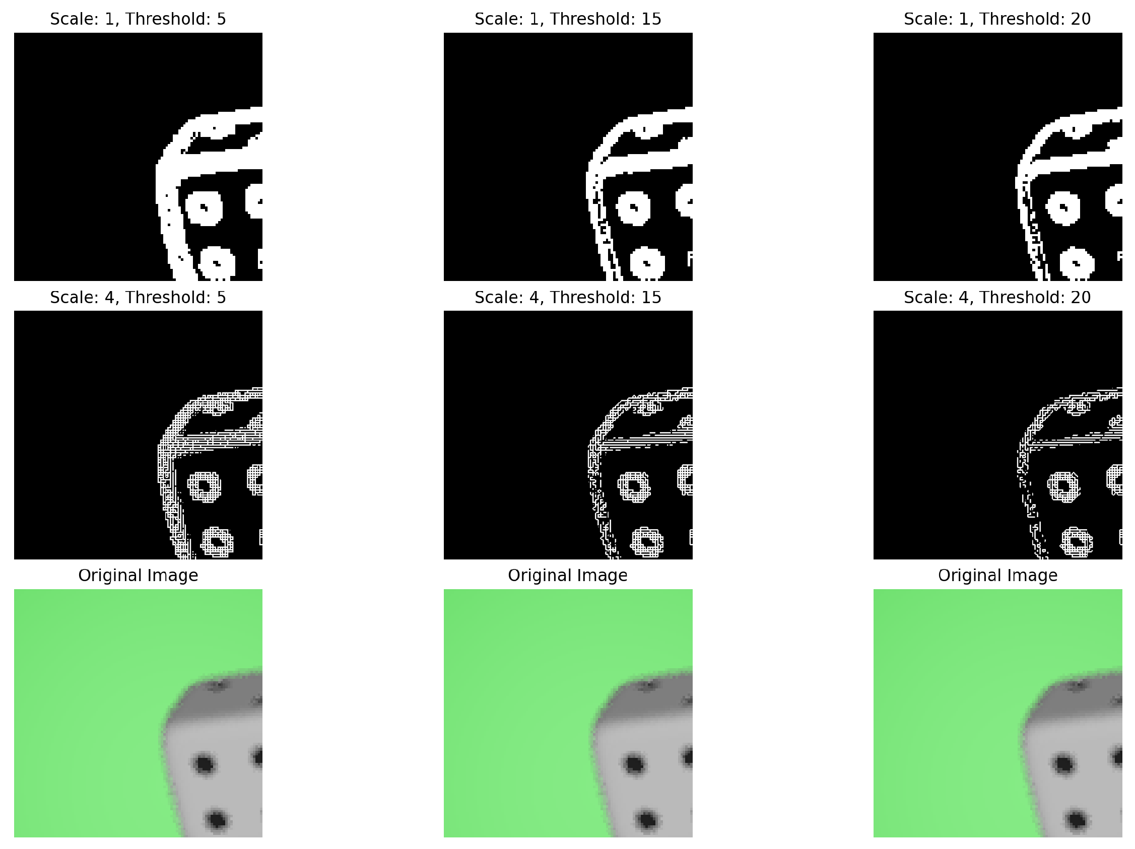
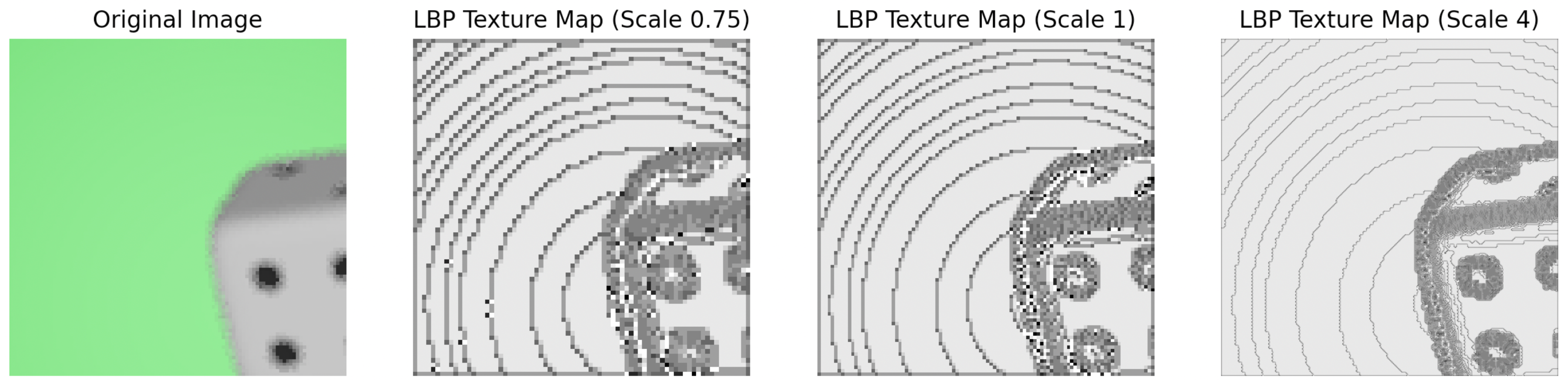
2.2.3. Multi-Resolution Content Analysis
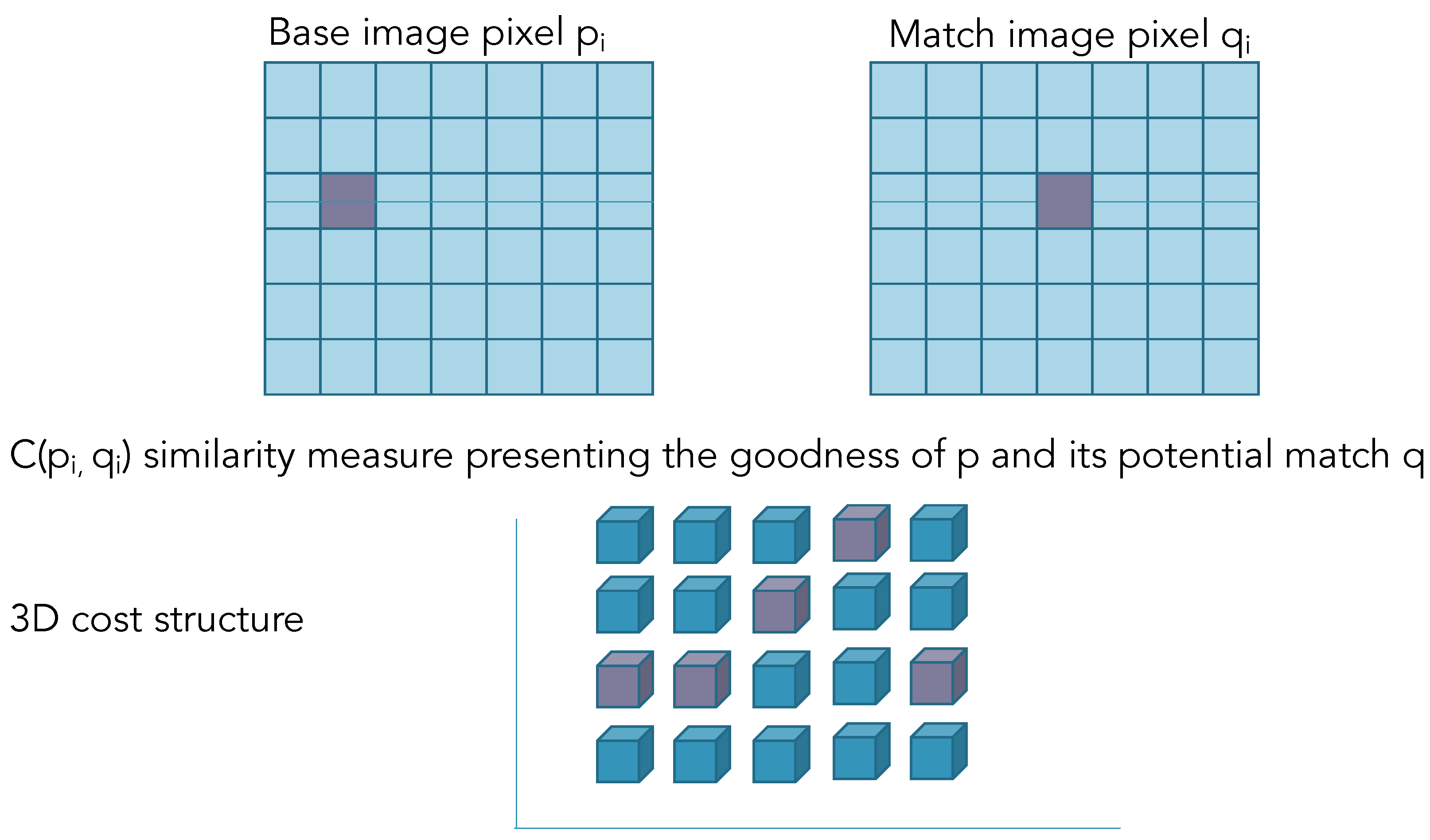
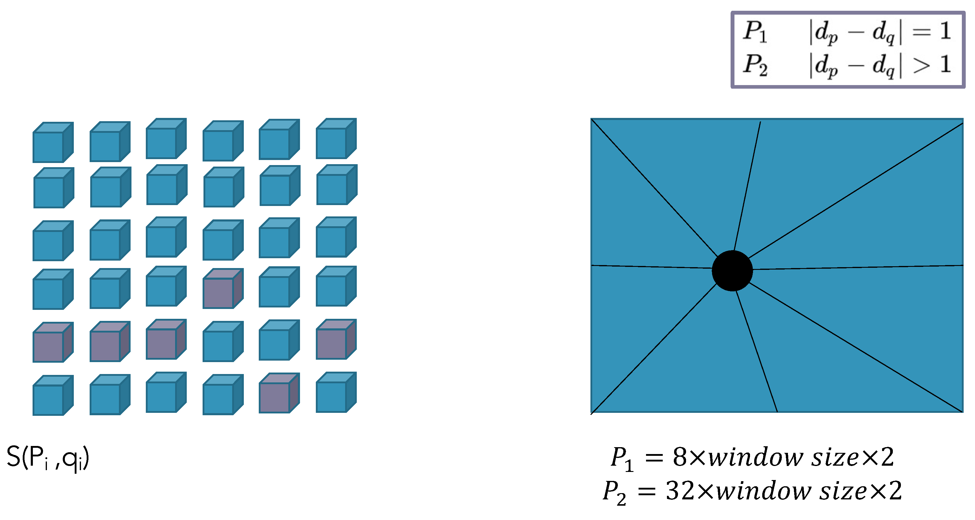
2.2.4. Multi-Resolution Multi-Window Disparity Estimation Using SGBM
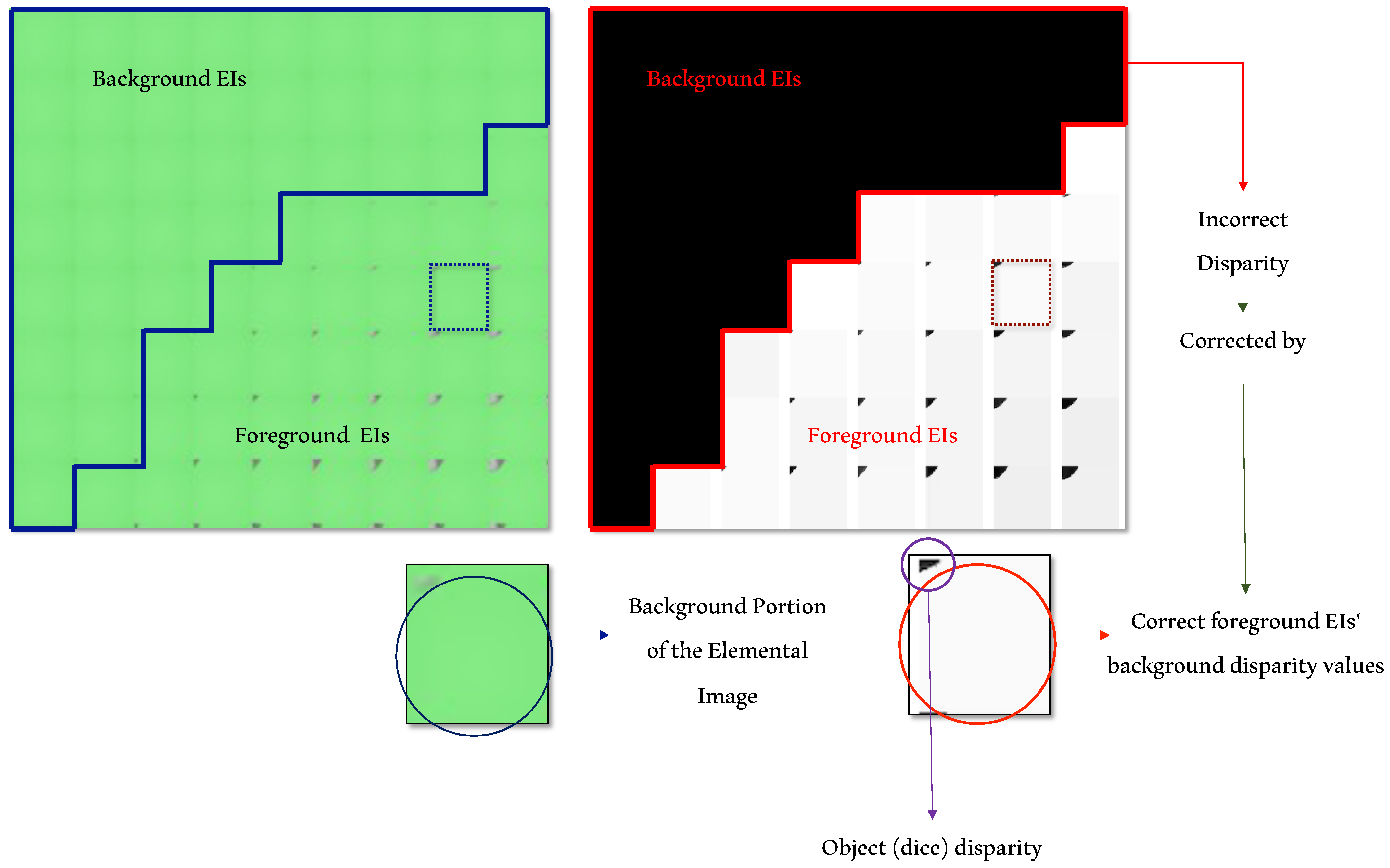
2.3. Background’s Disparity Correction
3. Evaluation
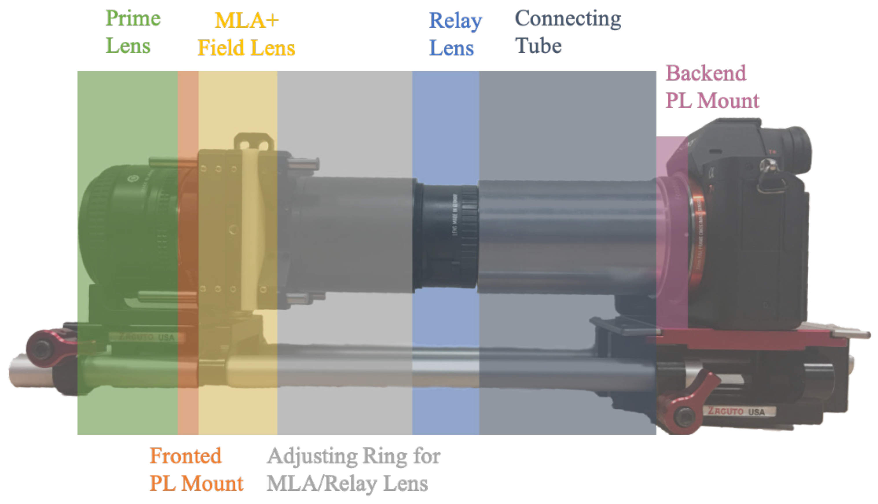
3.1. Dataset
3.2. Metrics
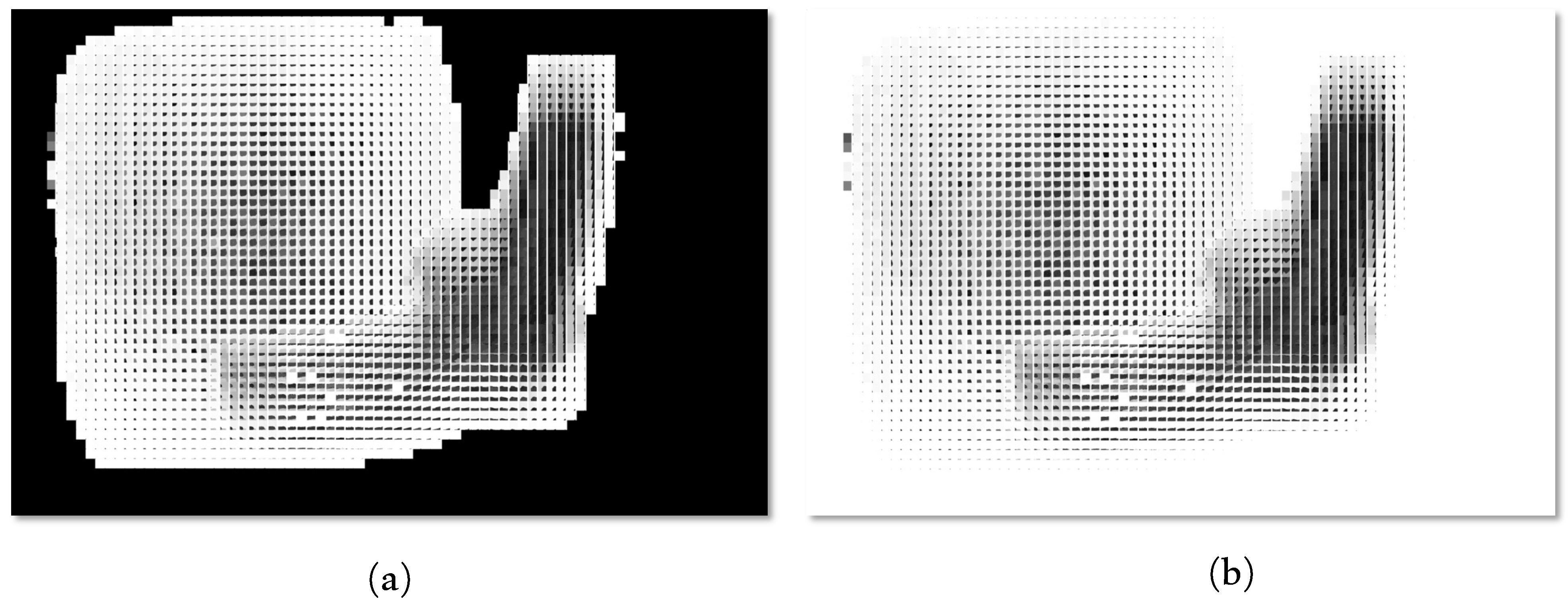
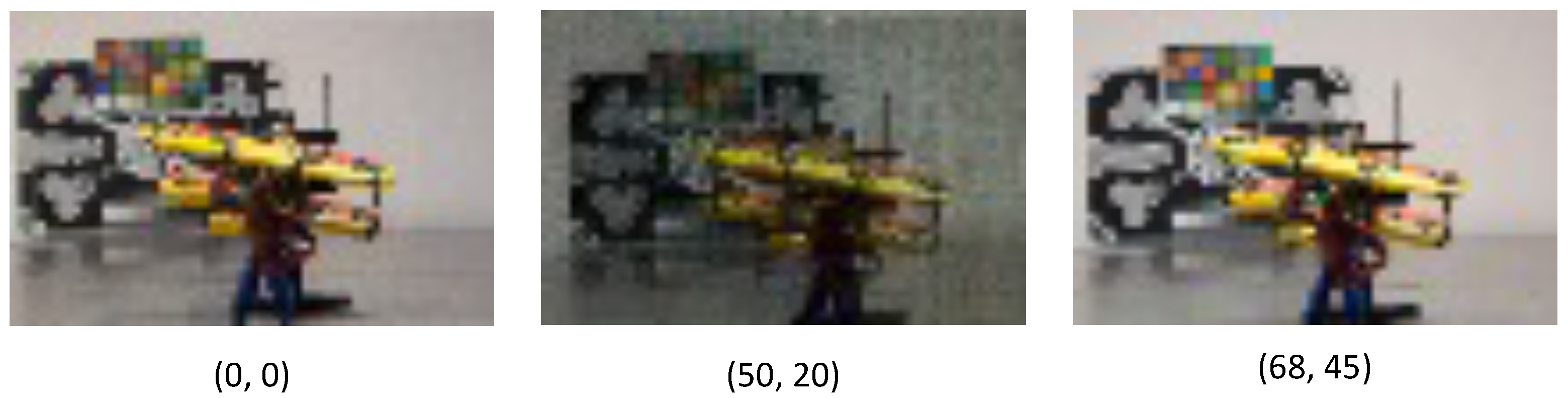
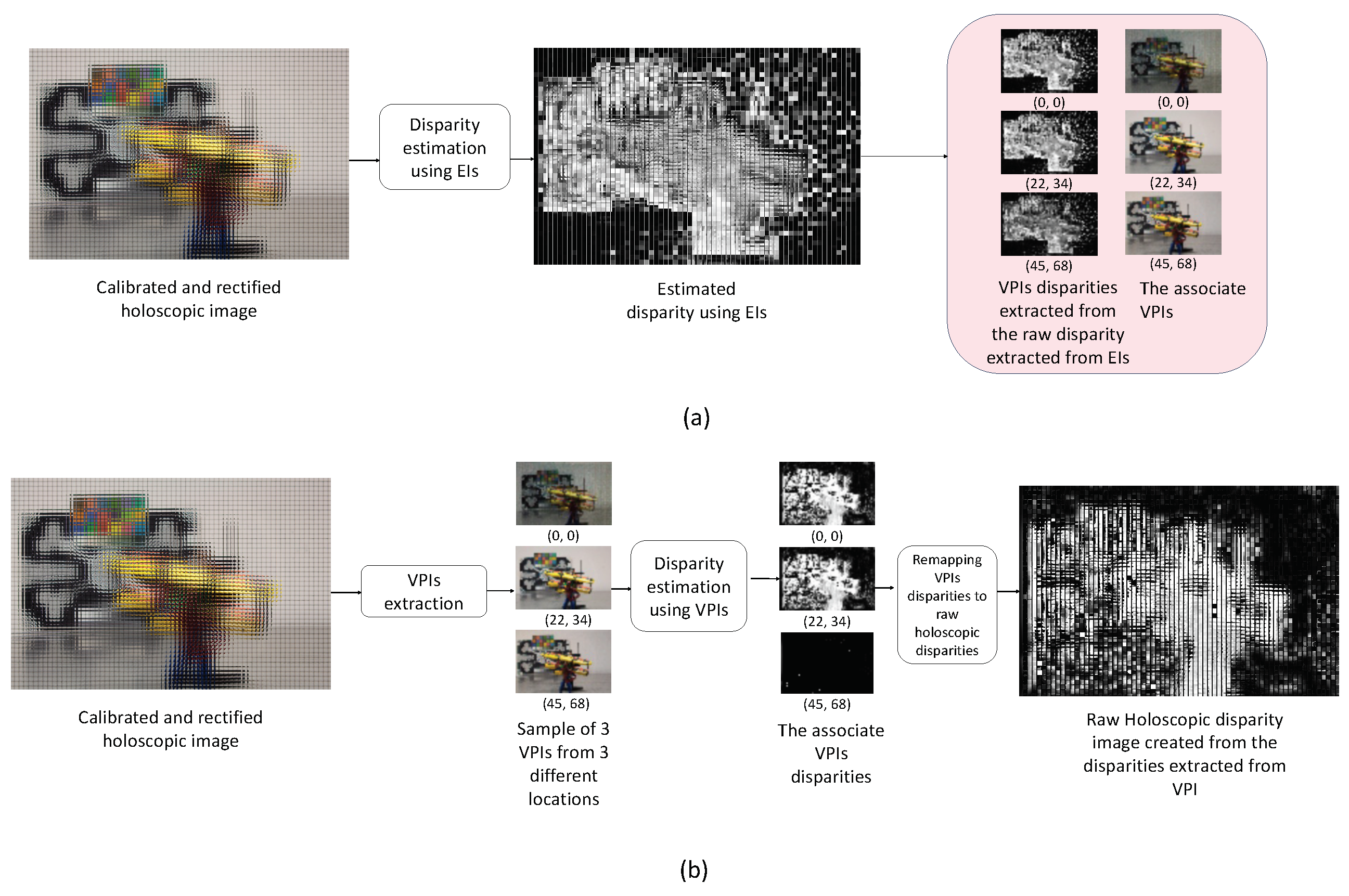
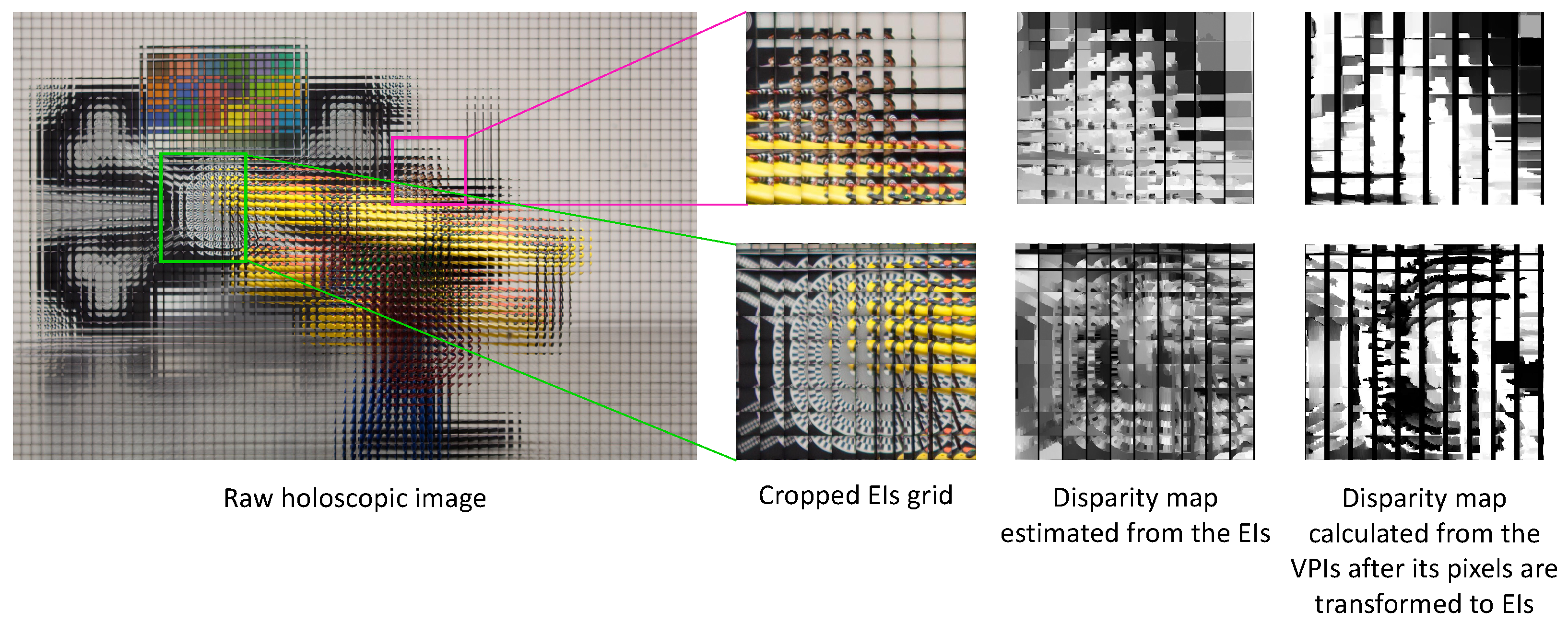
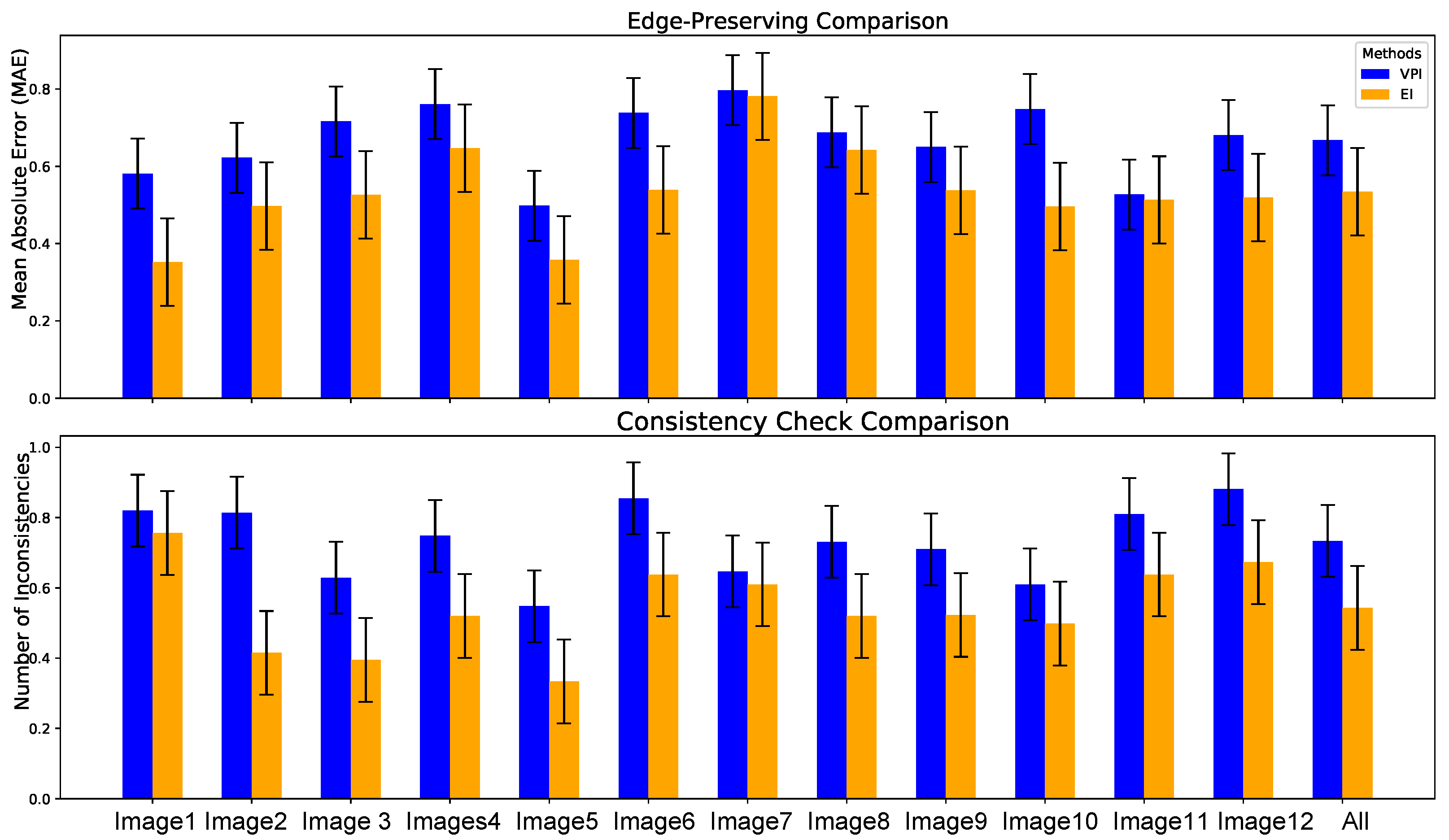
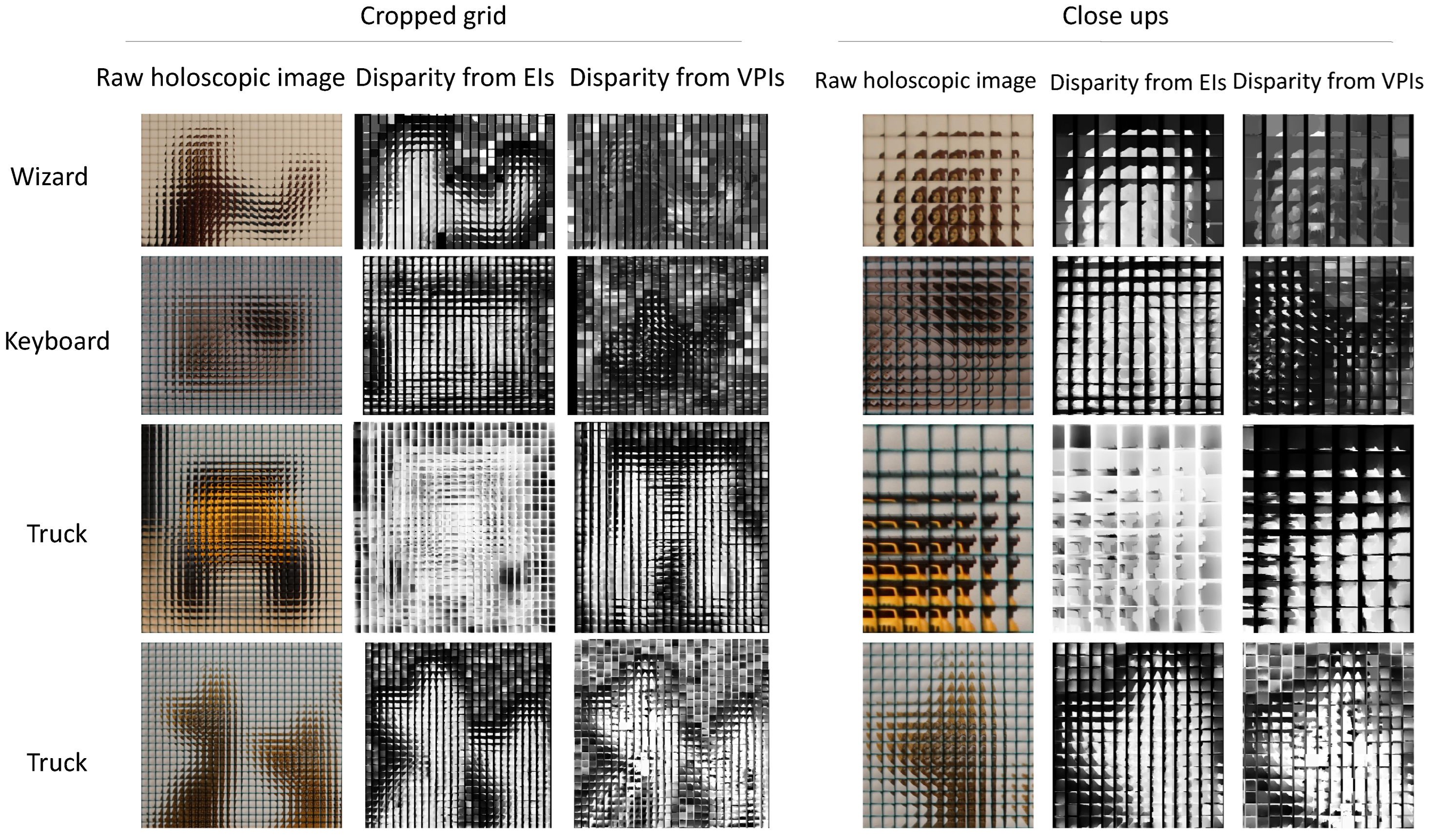
3.3. Elemental Image Compared to Viewpoint Image
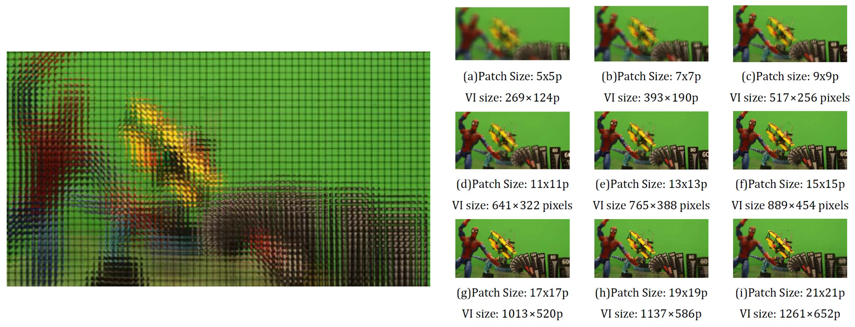
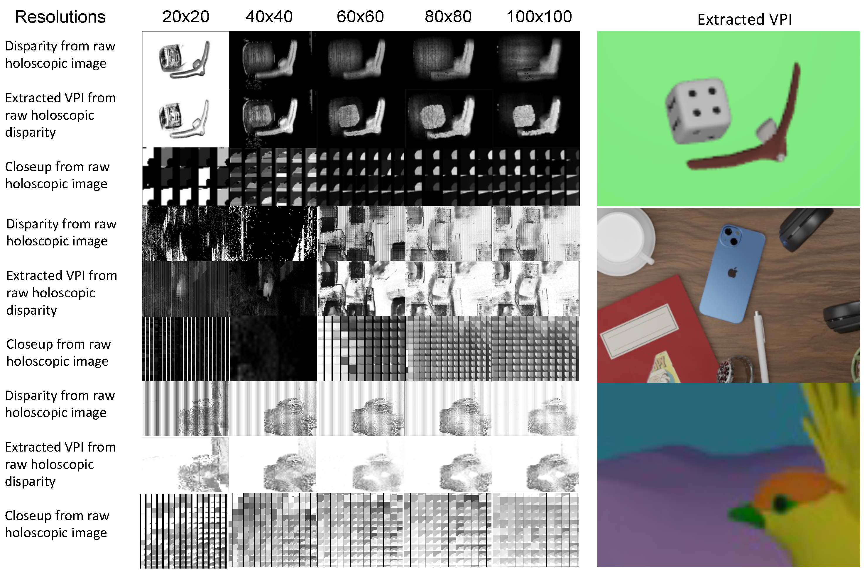
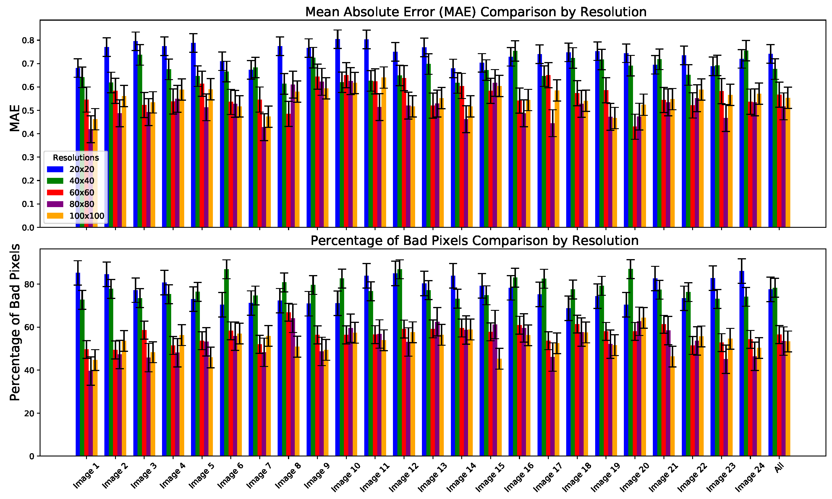
3.4. Elemental Image Compared to Viewpoint Image Resolution
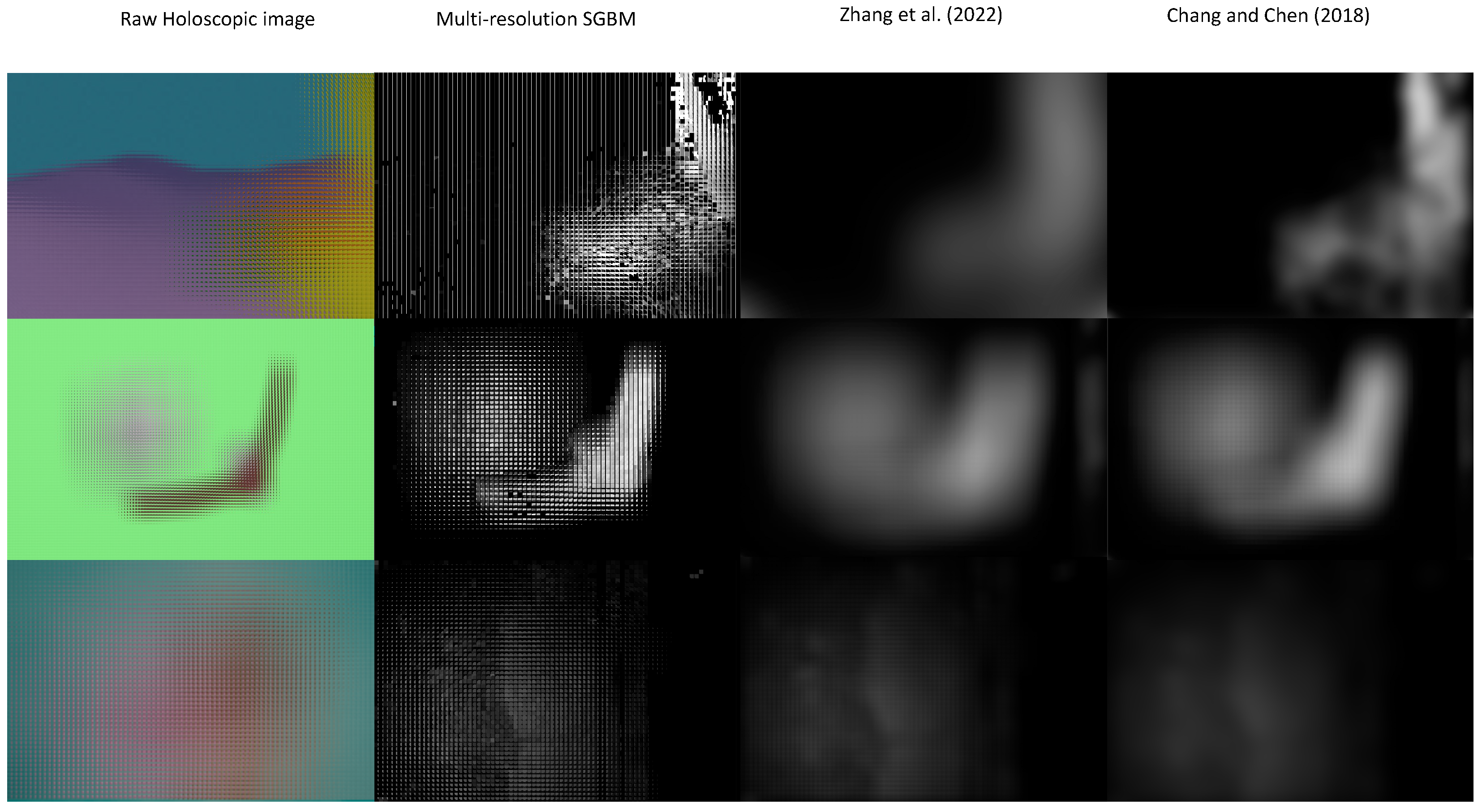
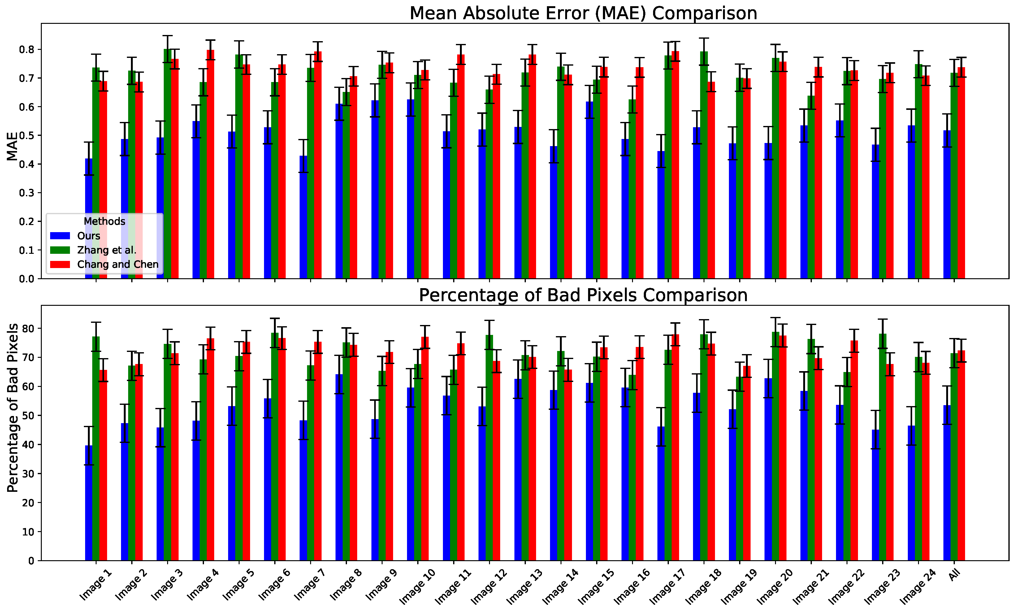
3.5. Comparative Analysis of Stereo-Matching Networks
4. Conclusions
Author Contributions
Funding
Data Availability Statement
Conflicts of Interest
References
- Cheng, Z.; Xiong, Z.; Chen, C.; Liu, D. Light field super-resolution: A benchmark. In Proceedings of the IEEE/CVF Conference on Computer Vision and Pattern Recognition Workshops, Long Beach, CA, USA, 16–17 June 2019. [Google Scholar]
- Lumsdaine, A.; Georgiev, T. Full resolution lightfield rendering. Indiana Univ. Adobe Syst. Tech. Rep. 2008, 91, 92. [Google Scholar]
- Lumsdaine, A.; Georgiev, T. The focused plenoptic camera. In Proceedings of the 2009 IEEE International Conference on Computational Photography (ICCP), San Francisco, CA, USA, 16–17 April 2009; IEEE: Piscataway, NJ, USA, 2009; pp. 1–8. [Google Scholar]
- Georgiev, T.; Lumsdaine, A. Reducing plenoptic camera artifacts. Comput. Graph. Forum 2010, 29, 1955–1968. [Google Scholar] [CrossRef]
- Ng, R.; Levoy, M.; Brédif, M.; Duval, G.; Horowitz, M.; Hanrahan, P. Light field photography with a hand-held plenoptic camera. Comput. Sci. Tech. Rep. CSTR 2005, 2, 1–11. [Google Scholar]
- Kinoshita, T.; Ono, S. Depth estimation from 4D light field videos. In Proceedings of the International Workshop on Advanced Imaging Technology (IWAIT) 2021, Online, 5–6 January 2021; SPIE: Paris, France, 2021; Volume 11766, pp. 56–61. [Google Scholar]
- Mousavi, M.; Khanal, A.; Estrada, R. Ai playground: Unreal engine-based data ablation tool for deep learning. In Proceedings of the International Symposium on Visual Computing, San Diego, CA, USA, 5–7 October 2020; Springer: Berlin/Heidelberg, Germany, 2020; pp. 518–532. [Google Scholar]
- Tankus, A.; Kiryati, N. Photometric stereo under perspective projection. In Proceedings of the Tenth IEEE International Conference on Computer Vision (ICCV’05), Beijing, China, 17–21 October 2005; IEEE: Piscataway, NJ, USA, 2005; Volume 1, pp. 611–616. [Google Scholar]
- Park, J.H.; Baasantseren, G.; Kim, N.; Park, G.; Kang, J.M.; Lee, B. View image generation in perspective and orthographic projection geometry based on integral imaging. Opt. Express 2008, 16, 8800–8813. [Google Scholar] [CrossRef] [PubMed]
- Eagle, R.; Hogervorst, M. The role of perspective information in the recovery of 3D structure-from-motion. Vis. Res. 1999, 39, 1713–1722. [Google Scholar] [CrossRef] [PubMed]
- Thomas, G.A.; Stevens, R.F. Processing of Images for 3D Display. US Patent 6,798,409, 28 September 2004. [Google Scholar]
- Hirschmuller, H. Stereo processing by semiglobal matching and mutual information. IEEE Trans. Pattern Anal. Mach. Intell. 2007, 30, 328–341. [Google Scholar] [CrossRef] [PubMed]
- Elad, M. On the origin of the bilateral filter and ways to improve it. IEEE Trans. Image Process. 2002, 11, 1141–1151. [Google Scholar] [CrossRef]
- Buades, A.; Facciolo, G. Reliable multiscale and multiwindow stereo matching. SIAM J. Imaging Sci. 2015, 8, 888–915. [Google Scholar] [CrossRef]
- Miangoleh, S.M.H.; Dille, S.; Mai, L.; Paris, S.; Aksoy, Y. Boosting monocular depth estimation models to high-resolution via content-adaptive multi-resolution merging. In Proceedings of the IEEE/CVF Conference on Computer Vision and Pattern Recognition, Nashville, TN, USA, 20–25 June 2021; pp. 9685–9694. [Google Scholar]
- Keys, R. Cubic convolution interpolation for digital image processing. IEEE Trans. Acoust. Speech Signal Process. 1981, 29, 1153–1160. [Google Scholar] [CrossRef]
- Almatrouk, B.; Meng, H.; Swash, M.R. Disparity estimation from holoscopic elemental images. In Proceedings of the International Conference on Natural Computation, Fuzzy Systems and Knowledge Discovery, Xi’an, China, 1–3 August 2020; Springer: Berlin/Heidelberg, Germany, 2020; pp. 1106–1113. [Google Scholar]
- Liu, W.; Chen, X.; Shen, C.; Liu, Z.; Yang, J. Semi-global weighted least squares in image filtering. In Proceedings of the Proceedings of the IEEE International Conference on Computer Vision, Venice, Italy, 22–29 October 2017; pp. 5861–5869.
- Alzu’bi, A.; Amira, A.; Ramzan, N. Semantic content-based image retrieval: A comprehensive study. J. Vis. Commun. Image Represent. 2015, 32, 20–54. [Google Scholar] [CrossRef]
- Rublee, E.; Rabaud, V.; Konolige, K.; Bradski, G.R. ORB: An efficient alternative to SIFT or SURF. In Proceedings of the ICCV, Barcelona, Spain, 6–13 November 2011; Volume 11, p. 2. [Google Scholar]
- Almatrouk, B.; Meng, H.; Aondoakaa, A.; Swash, R. A New Raw Holoscopic Image Simulator and Data Generation. In Proceedings of the 2023 8th International Conference on Image, Vision and Computing (ICIVC), Dalian, China, 27–29 July 2023; IEEE: Piscataway, NJ, USA, 2023; pp. 489–494. [Google Scholar]
- Zhang, J.; Wang, X.; Bai, X.; Wang, C.; Huang, L.; Chen, Y.; Gu, L.; Zhou, J.; Harada, T.; Hancock, E.R. Revisiting domain generalized stereo matching networks from a feature consistency perspective. In Proceedings of the IEEE/CVF Conference on Computer Vision and Pattern Recognition, New Orleans, LA, USA, 18–24 June 2022; pp. 13001–13011. [Google Scholar]
- Chang, J.R.; Chen, Y.S. Pyramid stereo matching network. In Proceedings of the IEEE Conference on Computer Vision and Pattern Recognition, Salt Lake City, UT, USA, 18–23 June 2018; pp. 5410–5418. [Google Scholar]


| EI Slice Resolution | |||||
|---|---|---|---|---|---|
| Original Resolution |  |  |  |  |  |
| Scaled-Down () |  |  |  |  |  |
| Scaled-Up () |  |  |  |  |  |
Disclaimer/Publisher’s Note: The statements, opinions and data contained in all publications are solely those of the individual author(s) and contributor(s) and not of MDPI and/or the editor(s). MDPI and/or the editor(s) disclaim responsibility for any injury to people or property resulting from any ideas, methods, instructions or products referred to in the content. |
© 2024 by the authors. Licensee MDPI, Basel, Switzerland. This article is an open access article distributed under the terms and conditions of the Creative Commons Attribution (CC BY) license (https://creativecommons.org/licenses/by/4.0/).
Share and Cite
Almatrouk, B.; Meng, H.; Swash, M.R. Holoscopic Elemental-Image-Based Disparity Estimation Using Multi-Scale, Multi-Window Semi-Global Block Matching. Appl. Sci. 2024, 14, 3335. https://doi.org/10.3390/app14083335
Almatrouk B, Meng H, Swash MR. Holoscopic Elemental-Image-Based Disparity Estimation Using Multi-Scale, Multi-Window Semi-Global Block Matching. Applied Sciences. 2024; 14(8):3335. https://doi.org/10.3390/app14083335
Chicago/Turabian StyleAlmatrouk, Bodor, Hongying Meng, and Mohammad Rafiq Swash. 2024. "Holoscopic Elemental-Image-Based Disparity Estimation Using Multi-Scale, Multi-Window Semi-Global Block Matching" Applied Sciences 14, no. 8: 3335. https://doi.org/10.3390/app14083335