Inversion of Sound Speed Field in Photoacoustic Imaging Based on Root Mean Square Propagation Algorithm

Abstract

The inaccuracy of inhomogeneous sound speed fields in photoacoustic imaging (PAI) can lead to the blurring and distortion of photoacoustic images. To solve this problem, conventional methods build speed models by using some a priori information or additional measuring equipment, which limits the application of PAI greatly. A data-driven speed field inversion method is proposed in this paper. It combines clustering with updates to the speed field. To reduce the complexity of the sound speed field model, the model is divided according to the similarity of the same tissue. The sound speed of the same tissue is regarded as a whole, which reduces the number of sound speed parameter solutions. Based on the simplified sound speed field model, the proposed method can adaptively adjust the step length of the sound speeds of various tissues by weight allocation. In this way, the updated amplitude of sound speeds of various tissues can be balanced and the accuracy of the sound speed field can be improved. A digital breast model is applied to verify the effectiveness of the proposed method. The results demonstrate that the method can build an appropriate speed field without additional information or equipment and improve the imaging performance of PAI.

1. Introduction

Photoacoustic imaging (PAI) is a rapidly developing hybrid imaging modality [1]. In recent years, it has made significant progress in structural imaging [2], molecular imaging [3], functional imaging [4] and so on. These fields provide technical support for the further realization of the early diagnosis of diseases. PAI is based on the photoacoustic effect. When the tissue to be measured is irradiated by a pulsed laser, the chromophore undergoes thermoelastic expansion. The local vibration of the tissue produces photoacoustic signals with outward propagation. These photoacoustic signals are collected by ultrasonic transducers. To ensure the accuracy of signals, the transducers currently applied in biological imaging technology have been improved with the help of nonlinear optics and machine learning [5]. Their performance has been significantly improved. After signal collection is completed, the photoacoustic image is obtained by signal inversion. The photoacoustic signal-generation, propagation and image-reconstruction processes are shown in Figure 1. A photoacoustic image can reflect the internal structure and function of biological tissues through differences in photoacoustic pressure [1,6].

In the practical application of PAI, the sound speed field is the key factor that affects the imaging performance. Its accuracy is essential for obtaining high-quality photoacoustic images. However, the sound speed field of biological tissue often presents inhomogeneous distribution. This inhomogeneity can significantly increase the difficulty of accurately estimating sound speed fields. The existing image reconstruction algorithms usually assume that a sound speed field is homogeneous to reduce the computational complexity [7]. This assumption may lead to serious deviations in the time-of-flight (TOF) of photoacoustic signals [8,9], which makes photoacoustic images blurred and distorted [10]. To avoid this situation, it is necessary to accurately estimate inhomogeneous sound speed fields in the process of image reconstruction.

Due to the serious impact of the inaccuracy of sound speed fields on the performance of PAI, how to accurately estimate sound speed fields has become an urgent problem to be solved in PAI. Some researchers proposed the transformation of the problem of estimating sound speed fields into a data clustering problem, which directly obtains the regional distribution of each tissue through photoacoustic pressure data. Wang et al. used K-means clustering to divide photoacoustic pressure data [11]. Yu et al. extracted the sparse spectrum of photoacoustic pressure data by basis tracing and processed the data by using the clustering value of the sparse spectrum and the clustering boundary [12]. Two methods used different clustering algorithms to obtain regional information about each tissue. However, they all rely on clinical data for sound speed assignment when estimating inhomogeneous sound speed fields. In addition, other strategies have been proposed by several researchers to construct sound speed fields. Huang et al. reported a joint reconstruction (JR) method based on an alternate optimization scheme, which can simultaneously obtain the sound speed distribution and absorbed light energy density of photoacoustic images [13]. Deep learning shows superior performance in improving imaging speed [14]. Some researchers also apply it to solve the problem of sound speed field estimation. Shan et al. proposed a synchronous reconstruction network (SR-Net), which combines deep learning with a joint reconstruction algorithm. It can obtain a relatively accurate sound speed field [15]. Merčep et al. adopted a strategy combining multi-modal imaging techniques. They developed a hybrid photoacoustic–ultrasonic imaging system that uses ultrasonic tomography (USCT) equipment to obtain sound speed distribution [16]. The above three methods can obtain relatively accurate inhomogeneous sound speed fields. However, the JR algorithm and USCT enhanced reconstruction algorithm have high computational costs and system complexity. To sum up, the existing sound speed field estimation methods are still dependent on prior information and additional measurement equipment, and some methods with superior performance have high computational complexity. The limitations of these methods greatly limit the application of PAI. To improve the performance of PAI, it is necessary to develop a speed field inversion method, which can realize the automatic optimization of sound speed fields with lower computational costs.

A speed field inversion method is proposed to reduce the influence of speed field inaccuracy on PAI in this paper. It combines clustering with updates to the speed field. The “K-means + Gaussian mixture model (GMM)” is used to fit the photoacoustic pressure data. This not only provides the regional location of various tissues for the construction of the speed field but also reduces the number of sound speed parameters to be estimated in the speed field model. Based on the simplified sound speed field model, the root mean square propagation (RMSprop) algorithm is introduced to optimize the sound speed of each tissue. To balance the updated sound speed amplitude of different tissues, the step length of each tissue is adaptively adjusted by weight allocation. This innovative advantage can effectively reduce the influence of interaction among tissues on the algorithm convergence process and ensure the convergence of the algorithm to the global optimal solution. Compared with existing methods, the proposed method can build appropriate speed fields without additional information or equipment. It adopts the iteration strategy as a whole. The clustering and RMSprop algorithm are used to alternately optimize the regional distribution and sound speed of each tissue, and the sound speed field is optimized automatically in a data-driven way.

2. Methods

2.1. The Influence of Inaccurate Sound Speed Fields on PAI

Assuming that biological tissue is a homogeneous medium, the basic equation of PAI can be expressed as follows [17]:

$${\nabla }^{2}p({\mathit{r}}_0,t)-\frac{1}{v^2}\frac{{\partial }^{2}p({\mathit{r}}_0,t)}{\partial t^2}=-\frac{\beta }{C}A(\mathit{r})\frac{\partial I(t)}{\partial t}.$$

(1)

In Equation (1), $p({\mathit{r}}_0, t)$ is the photoacoustic pressure received by the ultrasonic transducer at position ${\mathit{r}}_0$ at time t. v is the homogeneous sound speed. $\beta$ is the coefficient of thermal expansion. C is the specific heat capacity. $A(\mathit{r})$ represents the light absorption coefficient distribution function. $I\left(t\right)$ represents the time distribution function of the incident laser. Due to the short duration of the laser pulse, $I\left(t\right)$ can be replaced by an excitation pulse $\delta \left(t\right)$ approximation [17]. Using the Green function to solve $p({\mathit{r}}_0, t)$, the general relationship between photoacoustic pressure and the light absorption coefficient is obtained as follows [17]:

$$p({\mathit{r}}_0,t)=\frac{\beta }{4\pi C}\frac{\mathrm{d}}{\mathrm{d}t}{\displaystyle \int \frac{A(\mathit{r})}{\left|{\mathit{r}}_0-\mathit{r}\right|}\delta (t-\frac{\left|{\mathit{r}}_0-\mathit{r}\right|}{v})\mathrm{d}\mathit{r}}.$$

(2)

The temporal integral function of $p({\mathit{r}}_0, t)$ is introduced as follows:

$$G({\mathit{r}}_0,t)=\frac{4\pi C}{\beta }t{\displaystyle {\int }_0^{t}p({\mathit{r}}_0,t)}\mathrm{d}t.$$

(3)

Equation (2) is brought into Equation (3). The constant terms of the two formulas cancel, and the time derivative term $\mathrm{d}/\mathrm{d}t$ in Equation (2) cancels the time integral term ${\int }_0^t\mathrm{d}t$ in Equation (3), so Equation (4) is obtained, as follows:

$$G({\mathit{r}}_0,t)={\displaystyle \int A(\mathit{r})}\frac{1}{v}\delta (t-\frac{\left|{\mathit{r}}_0-\mathit{r}\right|}{v})\mathrm{d}\mathit{r},$$

(4)

where $G\left({\mathit{r}}_0, t\right)$ represents the spherical Radon transform of the $A\left(\mathit{r}\right)$; therefore, the photoacoustic image can be obtained by inverting the spherical Radon transform [18]. However, Equation (4) is only suitable for PAI under homogeneous sound speed fields.

When the presence of an inhomogeneous sound speed field is taken into account in PAI, the speed field causes photoacoustic signals to refract during propagation [19]. The sound speed at any position in this sound speed field can be set to $v\left({\mathit{r}}^{″}\right)$. The TOF of the photoacoustic signal is obtained by calculating the line integral of the reciprocal of the sound speed along the approximate propagation path as follows:

$$t_f(\mathit{r},{\mathit{r}}_0)={\displaystyle {\int }_l\frac{1}{v({\mathit{r}}^{″})}}\mathrm{d}l,\hspace{0.17em}\hspace{0.17em}l=\left|{\mathit{r}}_0-\mathit{r}\right|,$$

(5)

where $l$ is the distance from the sound source position r to the ultrasonic transducer ${\mathit{r}}_0$. Equation (5) is brought into Equation (2). The relationship between the photoacoustic pressure $p_{inh}({\mathit{r}}_0, t)$ obtained under the inhomogeneous sound speed field and $A\left(\mathit{r}\right)$ can be expressed as follows:

$$p_{inh}({\mathit{r}}_0,t)=\frac{\beta }{4\pi C}\frac{\mathrm{d}}{\mathrm{d}t}{\displaystyle \int \frac{A(\mathit{r})}{\left|{\mathit{r}}_0-\mathit{r}\right|}\delta (t-t_f(\mathit{r},{\mathit{r}}_0))\mathrm{d}\mathit{r}}.$$

(6)

Equations (5) and (6) are brought into Equation (3) as follows:

$$G_{inh}({\mathit{r}}_0,t)={\displaystyle \int A(\mathit{r})}\frac{t_f(\mathit{r},{\mathit{r}}_0)}{\left|{\mathit{r}}_0-\mathit{r}\right|}\delta (t-t_f(\mathit{r},{\mathit{r}}_0))\mathrm{d}\mathit{r},$$

(7)

where $G_{\mathit{inh}}({\mathit{r}}_0, t)$ is called the generalized Radon transformation of the A(r) in the inhomogeneous sound speed field. The image reconstruction process can be achieved by performing the inverse Radon transform on Equation (7) [18].

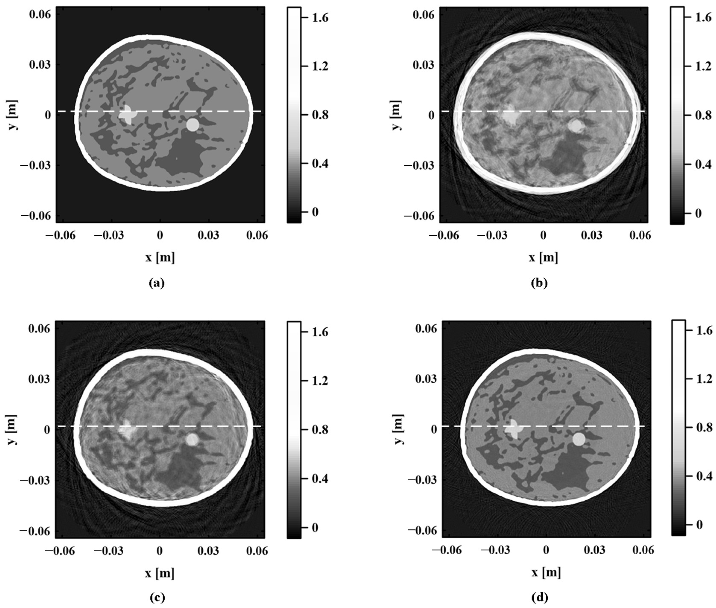
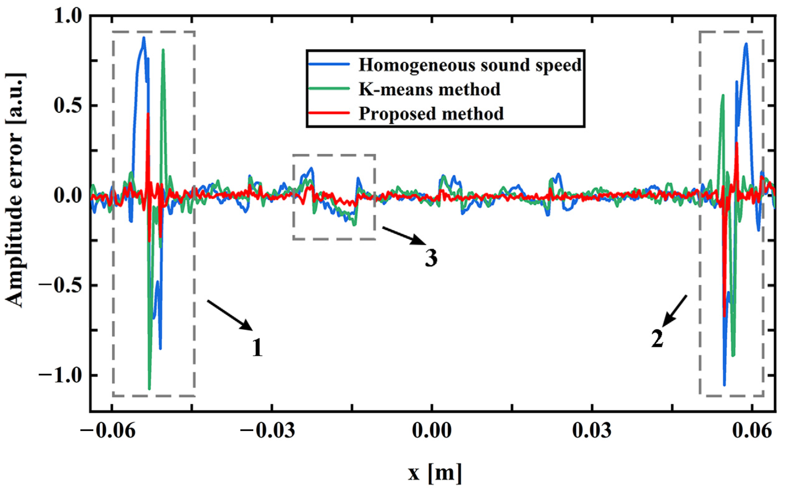
In the process of image reconstruction, the TOF is related to the propagation path of photoacoustic signal and depends on the sound speed distribution of biological tissue. If the inhomogeneous sound speed field is quite different from the real sound speed distribution in the reconstruction process, the TOF of photoacoustic signals will inevitably have serious errors. As shown in Equation (7), the change in TOF further leads to the failure of the photoacoustic signal to achieve focus at the target position, which makes the photoacoustic image appear as an artifact. The inaccuracy of the inhomogeneous sound speed field can seriously affect the quality of the photoacoustic image.

2.2. “K-Means + Gaussian Mixture Model” Clustering

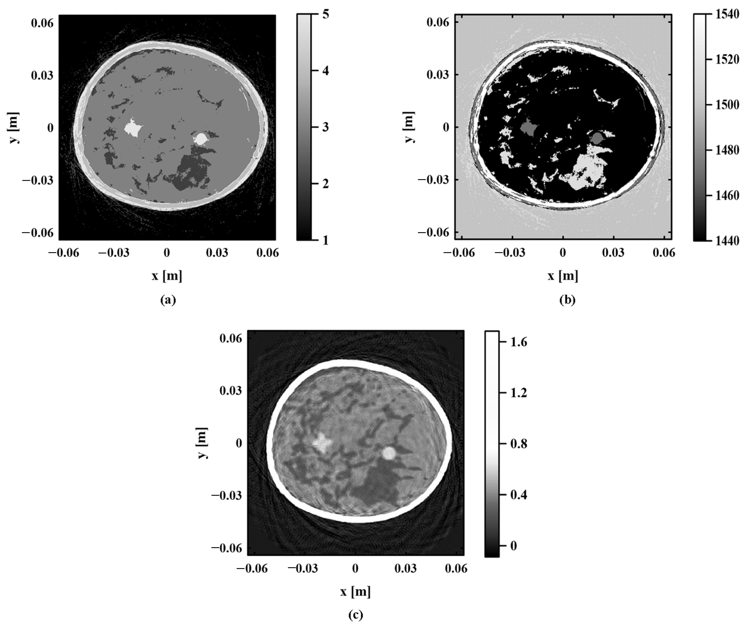
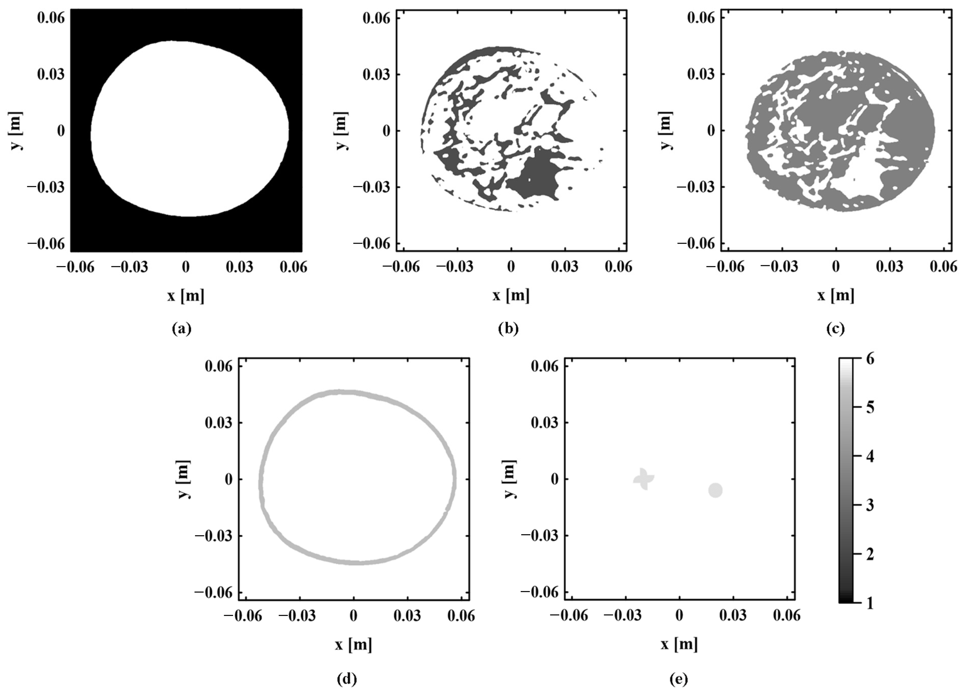
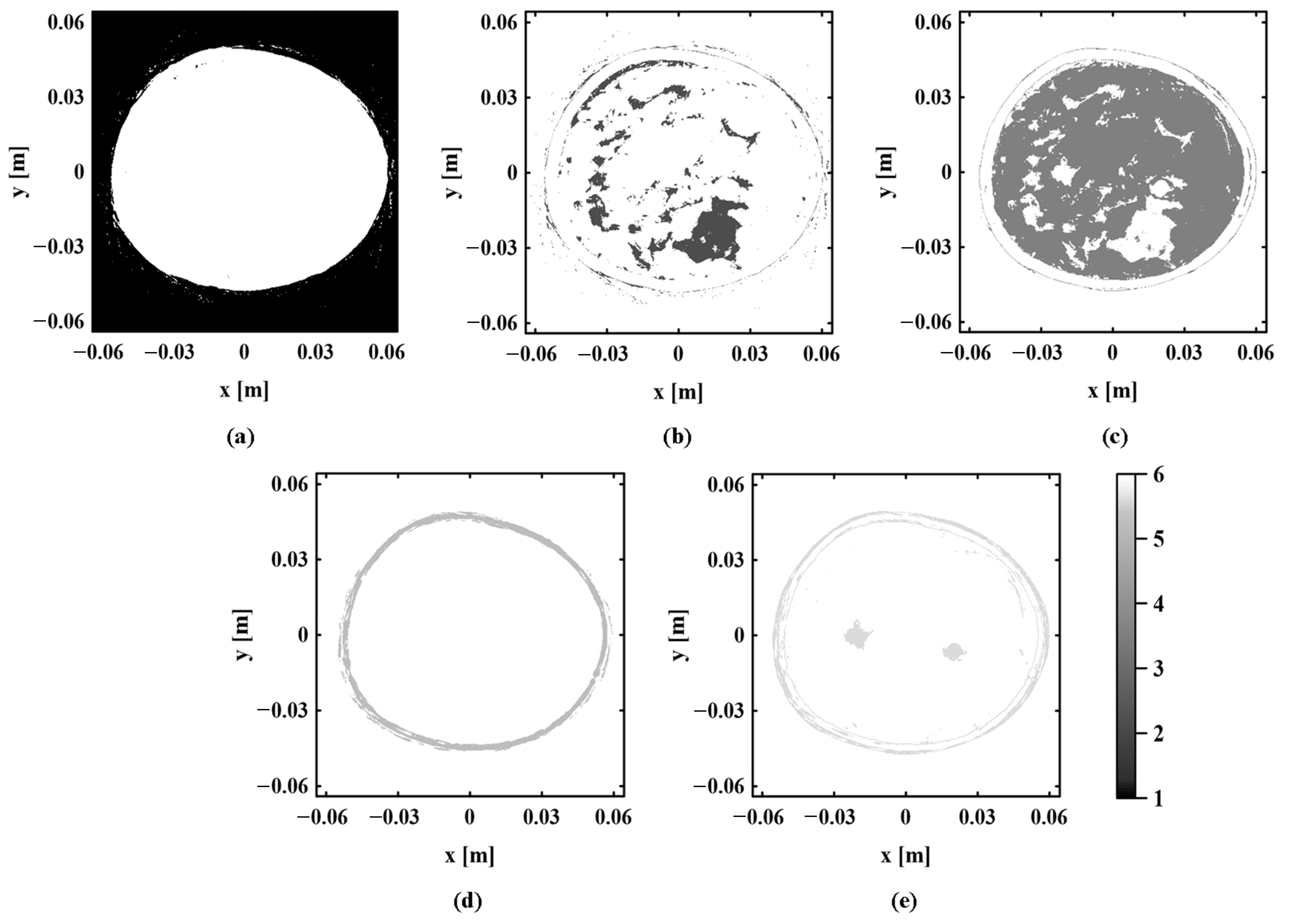
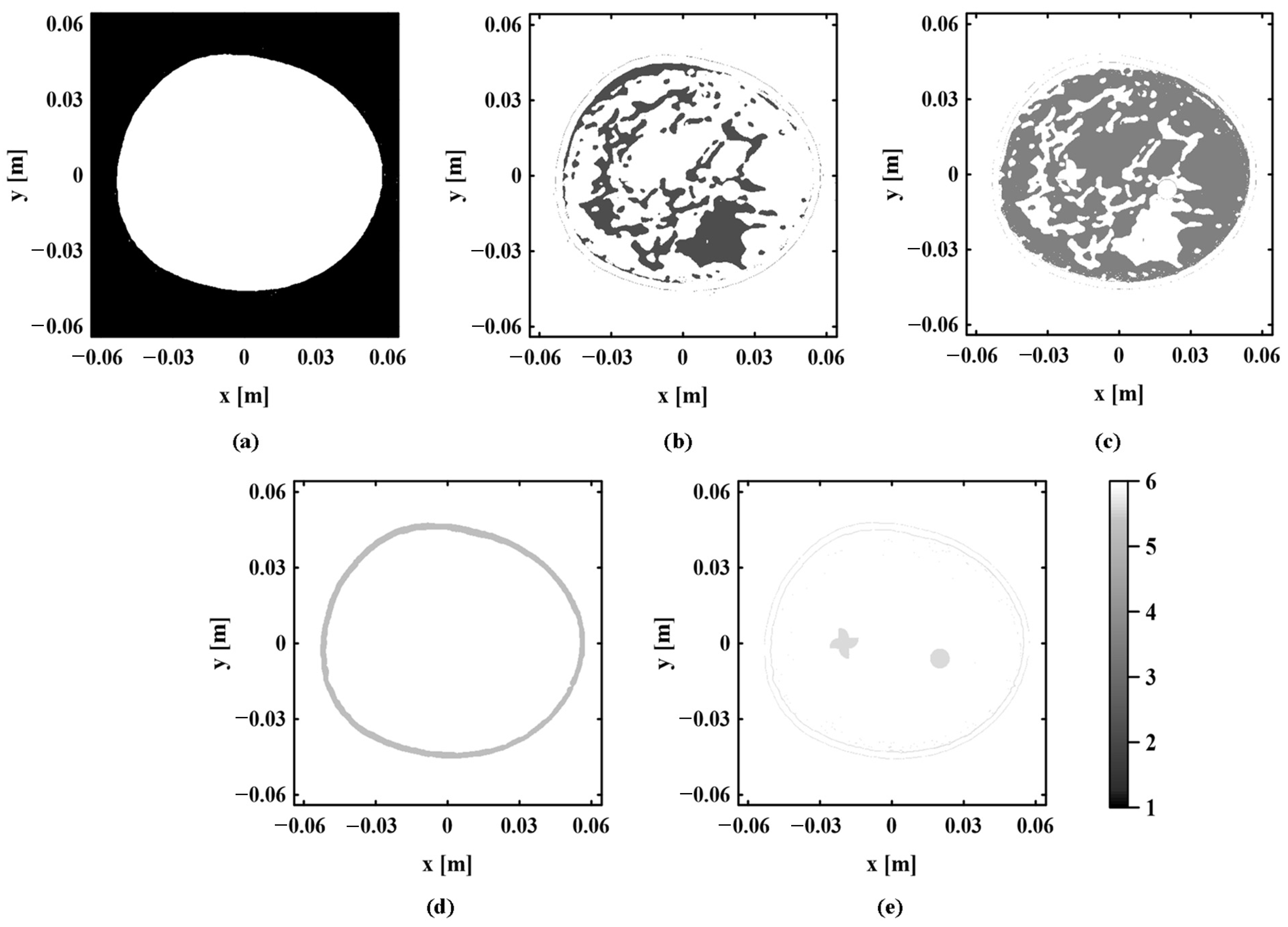
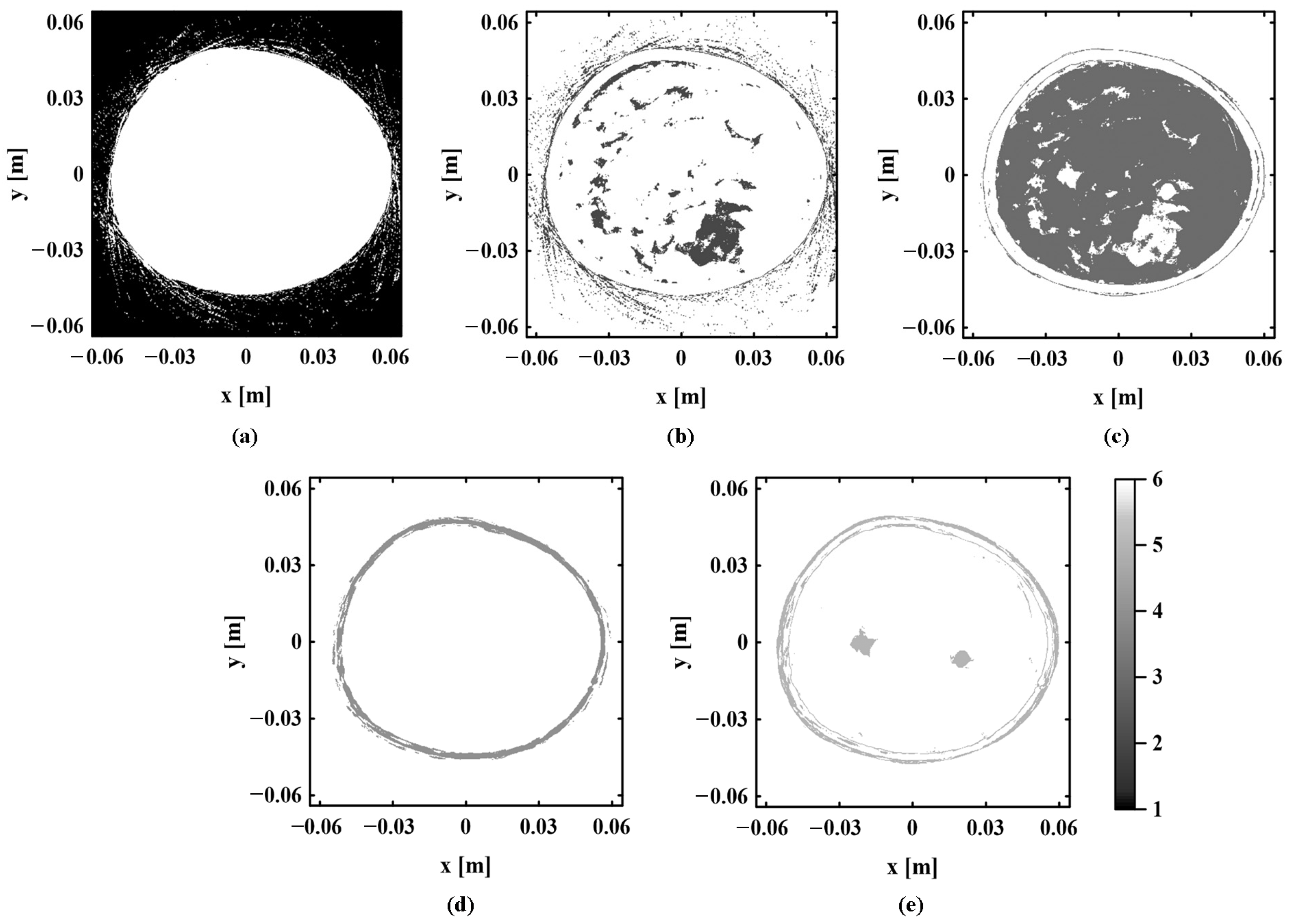
In PAI, the sound speed field is one of the important parameters that directly affect the accuracy and quality of imaging. It is necessary to accurately estimate the inhomogeneous sound speed field of biological tissues. Since identical tissues in biological tissues have similar properties, data clustering can be carried out according to the similarity between the photoacoustic pressure data to extract the regional location information about various tissues. The application of clustering regards the same tissue region of homogeneous sound speed as a whole. This reduces the number of sound speeds to be estimated in the inhomogeneous sound speed field and provides convenience for the further accurate estimation of sound speed distribution.

The internal structure of biological tissue is reflected through the photoacoustic pressure value of each pixel in a photoacoustic image. The photoacoustic pressure data are matrix data of $m\times n$. The sequence form is expressed as $P =\left\{p_1,{ p}_2,\cdots , p_N\right\}, N =m \times n$. The proposed method combining K-means and GMM is used to cluster the data. Compared with K-means or GMM, this hybrid clustering displays a significant improvement in clustering performance [20]. It can obtain more accurate regional location information. K-means is one of the most common clustering analysis algorithms, and its convergence speed is fast. The application of K-means to pre-process photoacoustic pressure data can provide relatively accurate initial parameters for GMM and improve computational efficiency. K-means belongs to hard clustering. It takes distance as the similarity index and calculates the distance between each data and the center of each cluster. Each datum is divided into the closest cluster.

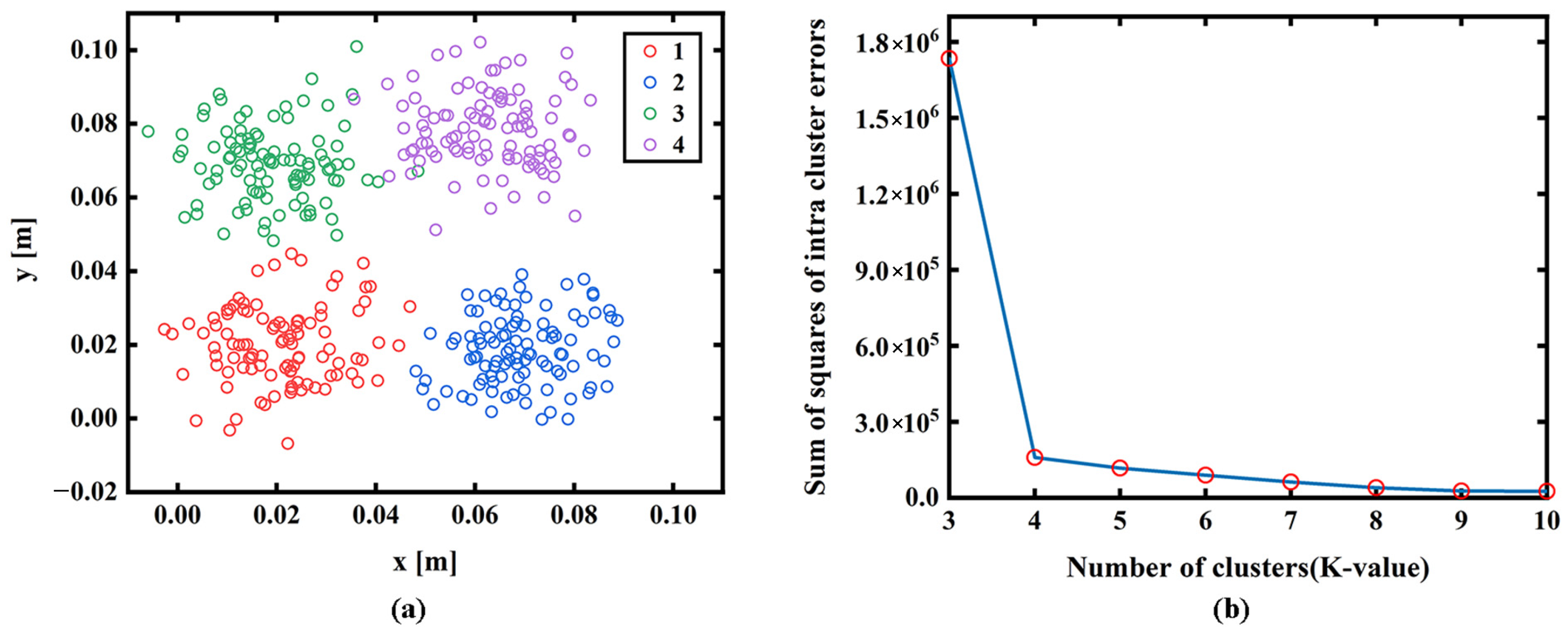
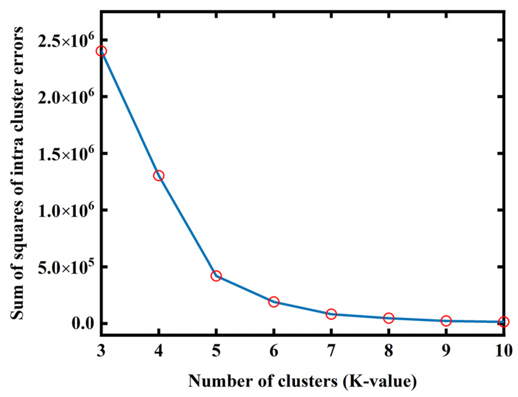
K-means needs to pre-specify the number of clusters, K, namely, the number of categories of the tissue. The elbow method is usually used to select the appropriate K value by comparing the sum of squared errors (SSE) of the clustering results corresponding to different clustering values. Four groups of randomly generated data in Figure 2a are taken as examples to explain the method as follows:

$$SSE={\displaystyle \sum _{k=1}^K{\displaystyle \sum _{i=1}^M{\left|p_{i,k}-{\mu }_k\right|}^2}}.$$

(8)

where K is the number of clusters, M represents the number of data contained in the kth cluster, $p_{i,k}$ represents the ith data point in the kth cluster and ${\mu }_k$ is the mean of all data in the kth cluster. The SSE value is used to evaluate the clustering result, which gradually decreases with the increase in clustering degree. As shown in Figure 2b, the SSE will decrease sharply when K reaches the most suitable clustering value and then plateau with increasing K values. The fitting map of SSE and K is the shape of an elbow, and the corresponding K value of the elbow is the best cluster number of the sample data. In addition, the elbow method can also provide the initial center point of each cluster for K-means to improve the accuracy of the clustering result.

The photoacoustic pressure data are trained several times by the elbow method. The most suitable clustering value K and the corresponding initial center are selected. They are brought into the K-means to obtain preliminary clustering results. Because K-means can only fit the data by spherical clusters, for biological tissues with complex distribution, the clustering result obtained by this algorithm can only roughly describe the regional distribution of various tissues. To obtain a more accurate tissue distribution, the GMM is selected to further iteratively optimize the rough clustering result. The GMM belongs to soft clustering. It makes clustering by calculating the posterior probability that the data belong to each Gaussian distribution [21]. Compared with hard clustering, this algorithm can divide the category of tissue boundary region more flexibly. The GMM can fit data through arbitrary ellipsoidal clusters, which are more suitable for dealing with the regional division of complex biological tissues.

However, the GMM is very sensitive to the setting of initial parameters, and the number of clusters needs to be set in advance. The clustering result of K-means can provide it with the initial values of these parameters, avoiding the influence of the randomness of the initial parameters on the GMM. The GMM is a parametric probabilistic model. This model is given as follows:

$$f(p_i)={\displaystyle {\sum }_{k=1}^K{a}_k{N}_k\left(p_i,{\mu }_k,{\Sigma }_k\right)}.$$

(9)

where $N_k(p_i,{\mu }_k, {\Sigma }_k)$ stands for the probability density function of the kth Gaussian distribution. $a_k$ is the weight coefficient, which represents the proportion of each type of tissue. ${\mu }_k$ is the mean value, which corresponds to the central position of the distribution of each tissue. ${\Sigma }_k$ is the variance, which describes the distribution of data around the mean value. When the GMM is applied to fit the photoacoustic pressure data, the data need to be allocated to K Gaussian distributions, and each Gaussian distribution corresponds to the distribution information of a class of tissues. The initial parameters are set based on the clustering result of K-means. The cluster center point of the kth cluster can be set directly to the initial mean value of the kth Gaussian distribution. The initial weight coefficient of the kth Gaussian distribution is obtained according to the proportion of the number of data M in the kth cluster to the total data. The initial mean and the number of data M are brought into Equation (10). The initial variance parameter of the kth Gaussian distribution can be obtained.

$${\Sigma }_{0,k}=\frac{{\displaystyle {\sum }_i^M(p_i-{\mu }_{0,k}){(p_i-{\mu }_{0,k})}^T}}{M}.$$

(10)

After the initial parameters of the GMM are obtained, the expectation–maximization (EM) algorithm is used to iteratively optimize these parameters to obtain a set of optimal model parameters. The posteriori probability is estimated by the current model parameters in E-step of the EM algorithm, namely, the probability that the data $p_i$ belong to the kth Gaussian distribution as follows [20]:

$${\gamma }_{i,k}^{new}=\frac{a_k{N}_k(p_i,{\mu }_k,{\Sigma }_k)}{{\displaystyle {\sum }_{k=1}^K{a}_k{N}_k(p_i,{\mu }_k,{\Sigma }_k)}}.$$

(11)

The updated model parameters are calculated through the M-step of the EM algorithm as follows:

$${\mu }_k^{new}=\frac{{\displaystyle {\sum }_i^N({\gamma }_{i,k}^{new}{p}_i)}}{{\displaystyle {\sum }_i^N{\gamma }_{i,k}^{new}}},$$

(12)

$${\Sigma }_k^{new}=\frac{{\displaystyle {\sum }_i^N{\gamma }_{i,k}^{new}(p_i-{\mu }_k^{new}){(p_i-{\mu }_k^{new})}^T}}{{\displaystyle {\sum }_i^N{\gamma }_{i,k}^{new}}},$$

(13)

$$a_k^{new}=\frac{{\displaystyle {\sum }_i^N{\gamma }_{i,k}^{new}}}{N}.$$

(14)

In Equation (14), N represents the total number of photoacoustic pressure data. From Equations (12)–(14), a set of more accurate model parameters can be obtained. The GMM described by the set of model parameters is closer to the real distribution of biological tissues. These parameters are used to calculate the log-likelihood function of the GMM as follows:

$$\ln f(p_i)={\displaystyle {\sum }_{i=1}^N\ln \left\{{\displaystyle {\sum }_{k=1}^K{a}_k^{new}{N}_k^{new}(p_i,{\mu }_k^{new},{\Sigma }_k^{new})}\right\}}.$$

(15)

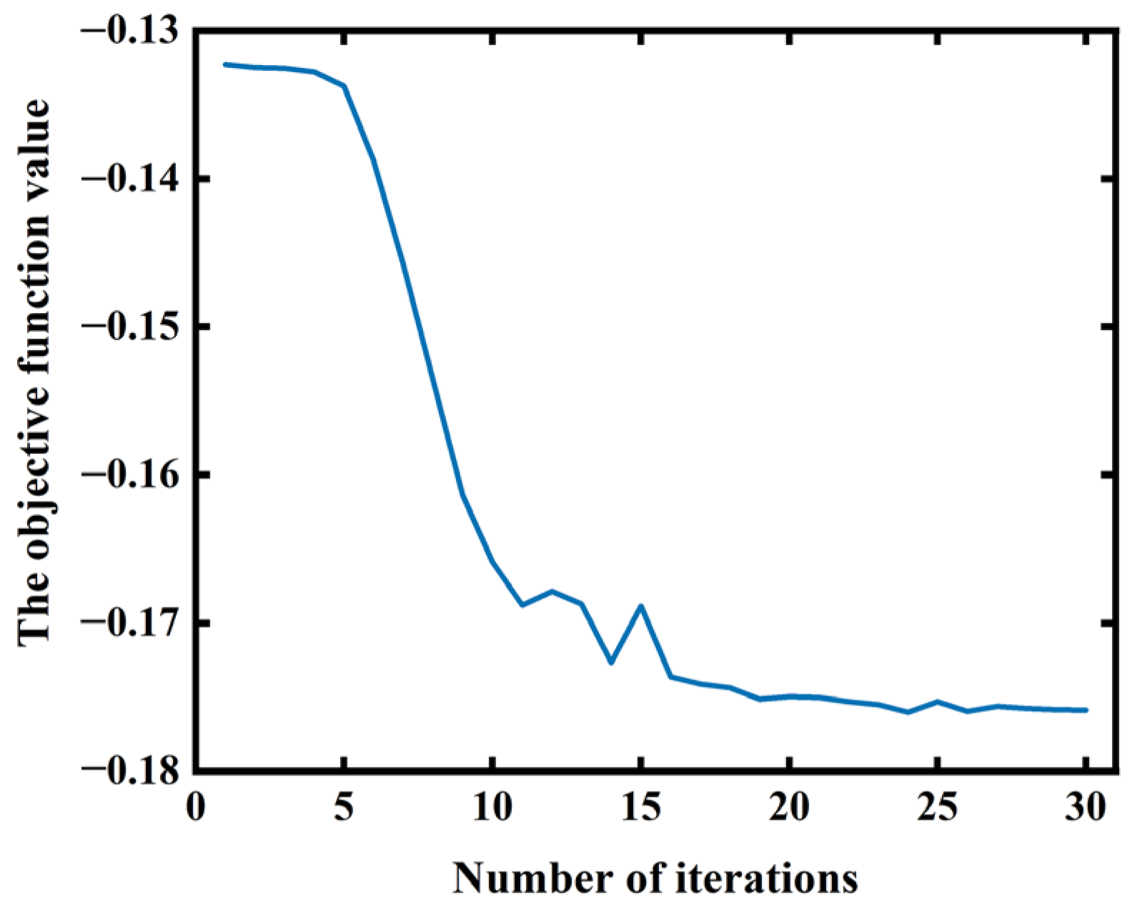
If the log-likelihood function does not converge, the model parameters need to return to E-step again for iterative updates. When the log-likelihood function of the model reaches the convergence state, the fitting effect of the GMM to the data also reaches its best. The current model parameter is the optimal model parameter. Each photoacoustic pressure datum is assigned to the Gaussian distribution with the largest probability according to the posteriori probability, and the clustering result can be obtained.

2.3. Root Mean Square Propagation Algorithm

“K-means + GMM” fits the photoacoustic pressure data into K Gaussian distributions; namely, the regional distribution information about K tissues is obtained. To further improve the accuracy of the sound speed field, it is necessary to search for more accurate sound speeds for each tissue based on regional distribution information. The clinical data information about biological tissues is usually selected for sound speed assignment in the reported methods. However, this method relies heavily on clinical data. Moreover, there are differences in tissue sound speeds among different individuals. The selection of sound speed based on clinical data may still be inaccurate. To avoid these problems, the RMSprop algorithm is used in this paper to realize the automatic optimization of the sound speed field. The RMSprop algorithm is an improved algorithm based on the gradient descent (GD) method, which continues the optimization strategy of the GD method. The fixed step length of the GD method is improved to the adaptive step length to improve the stability of the algorithm.

To highlight the improvement purpose of the RMSprop algorithm, the GD method is first introduced. The GD method is an optimization algorithm used to solve the extreme value problem of function [22]. It iteratively optimizes the independent variables of function by calculating the negative gradient direction of the objective function. It is hoped that the optimal solution of the corresponding independent variables can be obtained when the objective function converges. It is known that the purpose of correcting the inhomogeneous sound speed field is to improve the quality of photoacoustic images and make it closer to the real distribution of biological tissue. When the GD method is applied to solve the optimal sound speed, the function evaluating the quality of photoacoustic images can be set as the objective function. The sound speed of each tissue is the K parameter of the objective function. This method can identify the best search direction of the sound speed field and realize the automatic update of the sound speed of each tissue.

In the GD method, the initial sound speed vector and objective function are first set as follows:

$${\mathit{V}}_0={\left[v_{0,1}, v_{0,2},\cdots , v_{0,k},\cdots , v_{0,K}\right]}^T,$$

(16)

$$W_1=\sqrt{(\frac{p_{m+1,n}-p_{m-1,n}}{2}{)}^2+(\frac{p_{m,n+1}-p_{m,n-1}}{2}{)}^2},$$

(17)

$$F=-\frac{{\displaystyle {\sum }_{N_{W_2}}{W}_2}}{N_{W_2}}.$$

(18)

For the convenience of calculation, the sound speed of each tissue in the inhomogeneous sound speed field is formed into a sound speed vector in a fixed order. Equation (16) is the initial sound speed vector formed by the initial sound speed field. In Equation (17), $W_1$ represents the gradient value of the pixel at the (m,n) position. $p_{m,n}$ represents the photoacoustic pressure value of the pixel at the (m,n) position in the photoacoustic image. As shown in Equation (18), $W_2$ represents the photoacoustic pressure gradient values at each tissue boundary extracted from the $W_1$ data. $N_{W_2}$ represents the number of tissue boundary gradient values in $W_2$. The objective function F can be obtained by calculating the negative average of all the gradient values in $W_2$.

It is known that there are differences in photoacoustic pressure values in different tissue areas and the photoacoustic pressure values of the same type of tissue are very similar. When Equation (17) is applied to calculate the gradient, the gradient value of the pixels in the internal region of the tissue tends to be 0 due to the similarity of the tissues. The gradient value of the pixel in the tissue boundary region is determined by the photoacoustic pressure difference value of the tissue on both sides of the boundary. Its gradient value is larger relative to the gradient value inside the tissue. The photoacoustic pressure gradient value $W_2$ of each tissue boundary can be extracted by setting a threshold value. When the imaging effect is better, the photoacoustic pressure value in the tissue boundary area shows a “cliff-like” change. The gradient amplitude value of the boundary area extracted by the threshold is larger and the boundary is more accurate. When the imaging effect is poor, the photoacoustic pressure value in the tissue boundary region shows a gentle “stepped” change due to the possible blurring and artifacts in the image. This makes the gradient amplitude value lower in the border area. The above analysis shows that the gradient values of each tissue boundary in a photoacoustic image can reflect the quality of the image. When Equation (18) is applied to calculate the value of the objective function, the better the quality of the photoacoustic image, the smaller the value of the objective function.

Taking the sth iteration as an example, the gradient vector of the objective function at the sound speed vector ${\mathit{V}}_{\mathit{s}}$ is calculated. The gradient vector contains K derivatives. When the derivative of each type of tissue is calculated, only the sound speed of this tissue is changed and the sound speeds of other tissues remain unchanged, $\partial v_{s,k}$ is obtained. The value of the objective function before and after changing $v$ is calculated to obtain the D-value $\partial F_{s,k}$. The derivative of the kth tissue region is $g_{s,k}=\partial F_{s,k}/\partial v_{s,k}$. The gradient vector for this iteration is as follows:

$$\nabla \mathit{F}({\mathit{V}}_s)={\left[g_{s,1}, g_{s,2},\cdots , g_{s,k},\cdots , g_{s,K}\right]}^T.$$

(19)

The negative direction of the gradient vector is the direction with the fastest descent at ${\mathit{V}}_{\mathit{s}}$. Along this search direction, the sound speeds of various tissues are updated as follows:

$${\mathit{V}}_{s+1}={\mathit{V}}_s-\lambda \nabla \mathit{F}({\mathit{V}}_s).$$

(20)

where V_s+1 represents the updated sound speed vector and λ is the predefined constant step length.

The distribution size of different tissues in real biological tissues may be very different. When calculating the derivative of each tissue, the objective function is more sensitive to changes in the sound speed of the tissue with large regional distribution. This causes its derivative to differ from that of other tissues. In this case, if the fixed step length is applied to update the sound speed value, it may lead to large differences in the updated amplitude of the sound speed values of various tissues. The sound speed of tissue with large regional distribution may converge faster and even incorrectly compensate for sound speed errors in other tissues. It not only interferes with the updates to the sound speed of other tissues and seriously affects the stability of the convergence process, but also may trap the sound speed field into a local optimum. To solve this problem, the RMSprop algorithm is introduced to realize the improvement in the constant step length in the GD method. The RMSprop algorithm adaptively adjusts the step length of the sound speed of each tissue according to the weighted average of the square of the historical derivatives of the corresponding tissue [23]. If the derivative of the tissue is larger, the RMSprop algorithm will automatically reduce its step length. If the derivative of the tissue is smaller, its step length will automatically increase accordingly. The step length of adaptive adjustment can balance the amplitude of the sound speed update, which makes the convergence process more stable, and the accuracy of the sound speed field can be improved.

The RMSprop algorithm uses the idea of the exponential weighted moving average (EWMA) method to calculate the exponential mean of the latest h iterations of the derivative squared of various tissues, as shown in the following:

$${\theta }_{s,k}=\alpha {\theta }_{s-1,k}+(1-\alpha )g_{s,k}^2,$$

(21)

$$h=\frac{1}{1-\alpha }.$$

(22)

In Equation (21), ${\theta }_{s,k}$ is the exponential mean of the derivative squared of the kth tissue in the sth iteration. ${\theta }_{s-1,k}$ is the exponential mean of the derivative squared of the kth tissue in the (s−1)th iteration. $g_{s,k}^2$ represents the derivative squared of the kth tissue in the sth iteration. α represents the hyperparameter. h is the number of historical derivatives required to calculate the average value of the index. Based on the idea of the EWMA method, Equation (21) weights the derivative squared of the latest h iterations to control the contribution of the historical derivative squared to the exponential mean. The closer the derivative squared is to the current iteration, the greater the weight it multiplies. According to the weight size, the data information about derivative squared is extracted. The exponential mean obtained from Equation (21) provides reference data for the adaptive adjustment of step length.

In addition, the exponential mean calculated by the RMSprop algorithm in the early iteration may be inaccurate. To solve this problem, Equation (23) is applied to correct the deviation of the exponential mean to improve the accuracy of the early exponential mean.

$${\hat{\theta }}_{s,k}=\left\{\begin{array}{cc}\frac{{\theta }_{s,k}}{1-{\alpha }^s},& s<h,\\ \frac{{\theta }_{s,k}}{1-{\alpha }^h},& s\ge h.\end{array}\right.$$

(23)

In Equation (23), ${\hat{\theta }}_{s,k}$ is the corrected value of the exponential mean of the kth tissue in the sth iteration. The corrected value of the exponential mean of each tissue is calculated by Equation (23), which can provide the weight vector $\mathit{w}$ for adaptively adjusting the step length of the sound speed of each tissue.

$$\mathit{w}={\left[\frac{1}{\sqrt{{\hat{\theta }}_{s,1}}}, \frac{1}{\sqrt{{\hat{\theta }}_{s,2}}},\cdots , \frac{1}{\sqrt{{\hat{\theta }}_{s,k}}},\cdots , \frac{1}{\sqrt{{\hat{\theta }}_{s,K}}}\right]}^T.$$

(24)

The global step length is set to ${\lambda }_2$, and its initial value is ${\lambda }_{\mathit{initial}}$. To avoid the sound speed parameter producing a small range of oscillation in the later stage of iteration, the global step length slowly decays with iteration.

$${\lambda }_2={\lambda }_{initial}\cdot {\eta }^s.$$

(25)

where η is the attenuation coefficient of global step length. Along the direction of the negative gradient vector, various tissues use the corresponding step length to calculate the updated sound speed as follows:

$${\mathit{V}}_{s+1}={\mathit{V}}_s-{\lambda }_2\mathit{w}\odot \nabla \mathit{F}({\mathit{V}}_s).$$

(26)

where the ⊙ symbol is the Hadamard product, which refers to the new vector obtained by multiplying the elements at the corresponding positions of two vectors.

The RMSprop algorithm can balance the updated amplitude of sound speed by adaptively adjusting the step length of the sound speed of each tissue. It alleviates the interaction between various tissues in the process of updating sound speed. If a tissue with a large proportion reaches the convergence state, the small range change of its sound speed value may still have an impact on other tissues. To solve this problem, the sound speed values of several successive iterations after this tissue convergence can be selected to create an average, and the average value is taken as the optimal solution of this tissue’s sound speed. The sound speed value of this tissue is fixed as the optimal solution in the subsequent iterations to ensure the stability of the convergence process for other tissues.

In summary, the proposed algorithm optimizes the inhomogeneous sound speed field iteratively through two steps. “K-means + GMM” is used to update the regional location information about various tissues, and the RMSprop algorithm is applied to update the sound speed value of each tissue. When the sound speed values of various tissues begin to converge, the objective function values reach saturation. The final inhomogeneous sound speed field and photoacoustic image can be obtained.

3. Results and Analyses

3.1. Numerical Model and Configuration

A lifelike digital breast model is applied to verify the effectiveness of the proposed method. The digital breast model is generated from clinical magnetic resonance angiography data collected at Washington University School of Medicine in St. Louis. Magnetic resonance data are obtained from a breast with fibroglands in an extremely dense state [24]. Figure 3a shows the y−z slice of a dense fibrogland breast model at x = 4.0 $\times$ 10⁻² m. For better method validation, the microvessels are deleted from the original digital breast model, and two tumors are added at the border between fat and fibroglands. The digital breast model contains five components: water, fibroglands, fat, skin, and tumor. There is inhomogeneous sound speed distribution in this model. As shown in Figure 3a, the approximate locations of the five components are marked according to the serial numbers of each component specified in Table 1.

The digital breast model is simulated and reconstructed using the k-Wave toolbox in MATLAB R2019a [25]. The model is placed in a computational grid of 900 $\times$ 900. Its size is 0.18 m $\times$ 0.18 m. The two tumor sizes in the model are set as follows: tumor 1 is a circular tumor with a diameter of 8.0 $\times$ 10⁻³ m, and tumor 2 is an irregular tumor with a maximum diameter of 1.2 $\times$ 10⁻² m. Figure 3b shows the sound speed distribution map of the real sound speed field. The sound speed values of various components are set with reference to the sound speed range of biological tissues in the published literature, as shown in Table 1 [26]. The transducer is arranged in a ring array. A total of 800 ultrasonic transducers are uniformly arranged on a ring with a radius of 7.6 $\times$ 10⁻² m centered on the center of the computing grid to collect the photoacoustic signal in the forward simulation process. After obtaining the photoacoustic signal, the TR algorithm is applied to image the model. The use of the same computational grid for forward simulation and reconstruction during the calculation may mask potential errors; therefore, the reconstruction grid is set to 700 $\times$ 700 on the same model size.

Table 1. Real sound speed values of various components in the digital breast model [26].

Serial Number	Coupling Medium and Biological Tissues	Real Sound Speed (m/s)
1	water	1500.00
2	fibrogland	1515.00
3	fat	1440.00
4	skin	1540.00
5	tumor	1470.00

Table 1. Real sound speed values of various components in the digital breast model [26].

Serial Number	Coupling Medium and Biological Tissues	Real Sound Speed (m/s)
1	water	1500.00
2	fibrogland	1515.00
3	fat	1440.00
4	skin	1540.00
5	tumor	1470.00

3.2. Algorithm Implementation

In the proposed method, photoacoustic pressure data and photoacoustic image are obtained based on the homogeneous sound speed of 1495 m/s, as shown in Figure 4. This homogeneous sound speed value is selected from empirical values in the published literature. Comparing Figure 4 with the digital breast model in Figure 3a, it is observed that there are many artifacts in the photoacoustic image under a homogeneous sound speed. The boundaries of various tissues are blurred. The significant difference between the homogeneous and the real sound speed field seriously degrades the quality of the photoacoustic image. However, the photoacoustic pressure data obtained at a homogeneous sound speed can be used to provide initial regional position information about the sound speed field in the initial iteration. Figure 5 is a cluster deviation map of the photoacoustic pressure data at a homogeneous sound speed. As shown in Figure 5, the K value corresponding to the “elbow” is the optimal number of clusters, and the elbow method also provides the initial cluster center corresponding to K = 5.

“K-means + GMM” is used to divide the photoacoustic pressure data into five types of regions, and the initial clustering result is shown in Figure 6a. Figure 6b is the initial inhomogeneous sound speed field. In practical applications, the substance set in the background area is usually a coupling medium with a known sound speed. The coupling medium in the model is water, so the sound speed in this area can be fixed at 1500 m/s. The sound speeds of the other tissues to be measured are unknown, and the initial sound speed in these regions is set to 1495 m/s based on empirical values. The photoacoustic image shown in Figure 6c is obtained based on the sound speed field shown in Figure 6b. Since the location information and sound speed of each region are inaccurate in the initial inhomogeneous sound speed field, the boundaries of fat and fibrogland in Figure 6c are confused. The focusing effect of various tissues is poor, and in particular, the shape of tumor 2 is severely distorted.

Figure 7 shows the fitting curve of the objective function value and the number of iterations. It can be observed from this figure that there is a transient irregular oscillation phenomenon before the objective function value reaches saturation, which may be caused by the following two reasons:

(a)

In the process of solving, the step length of the updated sound speed of some tissues is too large, which affects the trend of gradient direction change and leads to the instability of the iterative process.

(b)

The objective function may be trapped in a local minimum, and the algorithm tries to escape from the local minimum, resulting in a transient oscillation of the objective function value [27].

The objective function value gradually converges in the middle and late iteration. This shows that the unique advantage of adaptively adjusting step length in the proposed method enhances the convergence of the algorithm. As shown in Figure 7, the objective function value of the photoacoustic image reaches saturation after 30 iterations.

Figure 8 illustrates the optimal clustering result, optimal sound speed field and photoacoustic image obtained by the proposed method. As shown in Figure 8b, the sound speed distribution of various tissues in the final obtained inhomogeneous sound speed field is very close to the real sound speed field. The photoacoustic image obtained based on this sound speed field is compared with the image at the homogeneous sound speed in Figure 4. The artifacts of the photoacoustic image in Figure 8c are significantly reduced, and the boundaries of various tissues are clearer.

To fully evaluate the effectiveness of the proposed method, the k-means sound speed estimation method is used to estimate the sound speed field of the digital breast model [11]. The result obtained is set as a control group for the proposed method. The k-means sound speed estimation method first performs Hilbert transformation on the photoacoustic image obtained at the homogeneous sound speed. This image is transformed into a unipolar photoacoustic image. After that, k-means is used to cluster the photoacoustic pressure values of each pixel in the unipolar photoacoustic image to obtain the regional distribution of each tissue. Finally, the sound speed of each tissue in the sound speed field is assigned according to the corresponding relationship between clinical data and clustering result. The photoacoustic image is obtained based on the updated sound speed field.

Figure 9 shows the results obtained by the k-means sound speed estimation method. Among them, the sound speed field shown in Figure 9b is obtained from the real sound speed values in Table 1. Since the regional distribution of each tissue in the sound speed field is quite different from the real distribution, the quality of the photoacoustic image obtained based on this sound speed field is not effectively improved.

3.3. Analysis of Clustering Results

To verify the effectiveness of the proposed method, the accuracy of the optimal sound speed field and the quality of the photoacoustic image are evaluated. It is known that the proposed method applies a clustering algorithm to characterize the regional distribution of various tissues in the sound speed field. As one of the factors affecting the accuracy of the speed field, it is necessary to evaluate the clustering results.

According to the clustering results obtained by the proposed method and the k-means sound speed estimation method, the regional distribution of each tissue is observed and compared one by one. Figure 10 shows the real regional distribution of each tissue in the digital breast model. Figure 11 and Figure 12, respectively, show the regional distribution of each tissue in the initial and optimal clustering maps obtained based on the proposed method. The regional distribution of each tissue in the cluster map obtained by the k-means sound speed estimation method is shown in Figure 13.

The regional distribution of each tissue in the initial and optimal clustering maps is compared with the corresponding real distribution. By observing Figure 10, Figure 11 and Figure 12, it can be seen that the regional boundary of each tissue in the optimal clustering map is clearer than that in the initial clustering map. Its regional distribution is closer to the real distribution of various tissues in the model. This shows that the proposed method can effectively improve the accuracy of each tissue distribution in the sound speed field through several iterations of cluster analysis. Next, the clustering results of the proposed method and k-means sound speed estimation method are compared by observing Figure 10, Figure 12 and Figure 13. The regional distribution of each tissue in the optimal clustering map is better than that of the k-means sound speed estimation method, which is closer to the real distribution. This indicates that the clustering performance of the proposed method is superior to that of the k-means sound speed estimation method.

To verify the clustering result as a whole, the clustering evaluation index is used to compare the clustering results obtained by the proposed method and the k-means sound speed estimation method. For clustering results, the higher the degree of intra-cluster aggregation and the greater the degree of inter-cluster dispersion, the better the clustering effect. The SSE index is used to evaluate the degree of intra-cluster aggregation of the clustering result. This index is calculated by the formula shown in Equation (8), which is the SSE of the intra-cluster sound pressure data with the intra-cluster mean. The SSE value is smaller, which indicates the intra-cluster aggregation of clustering result is better. The degree of inter-cluster dispersion is evaluated by the separation (SP) index, which represents the average distance between the center points (means) of various clusters as follows:

$$SP=\frac{2}{K\ast (K-1)}{\displaystyle \sum _{k_1=1}^K{\displaystyle \sum _{k_2=k_1+1}^K{‖{\mu }_{k_1}-{\mu }_{k_2}‖}_2}}.$$

(27)

where K represents the number of clusters in the clustering result. ${\mu }_{k_1}$ represents the mean of the k1st cluster. ${\mu }_{k_2}$ represents the mean of the k2nd cluster. The SP value is larger, which indicates the inter-cluster dispersion of clustering result is better.

Table 2. The SSE values and SP values of the clustering results obtained by the proposed method and the k-means sound speed estimation method.

Method	Proposed Method		K-Means Method
	Initial Clustering Result	Optimal Clustering Result
SSE	$2.1497\times {10}^7$	$9.0447\times {10}^6$	$4.7271\times {10}^7$
SP	0.1817	0.2697	0.1955

presents the SSE and SP values of the clustering results obtained by the two methods. In the clustering results obtained by the proposed method, the SSE value of the optimal clustering result is smaller than that of the initial clustering result, and the SP value is larger. Its clustering effect is better than the initial clustering result. This also shows that the proposed method can correct the regional distribution of each tissue in the sound speed field. Next, the SSE value and SP value of the optimal clustering result obtained by the proposed method are compared with the k-means sound speed estimation method. The results show that the SSE and SP values of the optimal clustering result are better than the k-means sound speed estimation method. The optimal clustering results obtained by the proposed method have a higher degree of intra-cluster aggregation and a greater degree of inter-cluster dispersion.

Whether observing and comparing the regional distribution of various tissues one by one or evaluating the overall clustering results through clustering indexes, the two comparison results show that the proposed method can significantly improve the regional distribution of each tissue in the sound speed field. Compared with the k-means sound speed estimation method, the optimal clustering result obtained by the proposed method is closer to the regional distribution of the real sound speed field, and its clustering performance is superior.

3.4. The Error Analysis of Sound Speed

The accuracy of the inhomogeneous sound speed field is further evaluated from the angle of sound speed error. The sound speeds of various tissues are extracted from the real, initial and optimal sound speed fields. The absolute error of the sound speed of each tissue in the initial and optimal inhomogeneous sound speed fields relative to the real sound speed is calculated. As shown in

Table 3. The absolute error of the sound speed of each tissue in the initial and optimal sound speed fields relative to the real sound speed.

Coupling Medium and Biological Tissues	Real Sound Speed (m/s)	Initial Sound Speed (m/s)		Optimal Sound Speed (m/s)
		Sound Speed	$∆{\mathit{v}}_1$	Sound Speed	$∆{\mathit{v}}_2$
water	1500.00	1500.00	0.00	1500.00	0.00
fibrogland	1515.00	1495.00	−20.00	1510.62	−4.38
fat	1440.00	1495.00	55.00	1440.68	0.68
skin	1540.00	1495.00	−45.00	1537.98	−2.02
tumor	1470.00	1495.00	25.00	1470.50	0.50

, $∆v_1$ represents the absolute error between the sound speed of each tissue in the initial sound speed field and the real sound speed. $\Delta v_2$ represents the absolute error between the sound speed of each tissue in the optimal sound speed field and the real sound speed. Comparing the absolute error in Table 3, it can be seen that the absolute values of the $\Delta v_2$ of various tissues are much smaller than the absolute value of $∆v_1$. These indicate that the sound speeds of various tissues in the optimal sound speed field are closer to the real sound speed. The proposed method can significantly improve the accuracy of the sound speed of each tissue.

The sound speed field obtained by the k-means sound speed estimation method is assigned according to the real sound speed values in Table 1. However, the sound speeds in the optimal sound speed field obtained by the proposed method still have small errors with the true sound speed values. Therefore, only from the angle of sound speed error, the accuracy of the sound speed of each tissue obtained by the proposed method is slightly worse than that of the k-means sound speed estimation method.

The above evaluation results show that the proposed method can significantly improve the accuracy of the inhomogeneous sound speed field from the two perspectives of clustering results and sound speed errors. In addition, the comparison results with the k-means sound speed estimation method show that the proposed method has better clustering performance. The region distribution of each tissue in the optimal sound speed field obtained by this method is more accurate. However, the sound speed error of each tissue is not completely eliminated, and the accuracy of the sound speed value is slightly worse than that of the k-means estimation method. In this case, the sound speed field obtained by the two methods is unable to accurately judge which one has better quality. The photoacoustic images based on these two sound speed fields need to be evaluated to further prove whether the sound speed field obtained by the proposed method is more accurate.

3.5. The Quality Evaluation of Photoacoustic Image

The performance of the proposed method is further verified by evaluating the quality of photoacoustic images. The photoacoustic image obtained by the proposed method is compared with the images obtained based on a homogeneous sound speed field and the k-means sound speed estimation method. Figure 14 gathers the real digital breast model and the photoacoustic images obtained by the above three sound speed estimation methods. As shown in Figure 14b, there are many artifacts in the photoacoustic image obtained based on the homogeneous sound speed field, and the boundaries of each tissue are blurred. The shape of the tumor tissue is distorted and the position of the skin tissue is obviously deviated. Figure 14c shows the photoacoustic image obtained based on the k-means sound speed estimation method. The artifacts of this image are reduced and the shape of the tumor tissue is closer to a real tumor shape. However, the sharpness of the image is still poor, and many details of the model are not shown. The photoacoustic image obtained by the proposed method is shown in Figure 14d. Compared with the photoacoustic images obtained by the other two methods, the sharpness of this image is significantly improved. Not only is the position of each tissue accurately located, but also, the details in the image are very clear.

The quality of the photoacoustic image is quantitatively evaluated by the photoacoustic pressure amplitude error map. In Figure 14, the photoacoustic pressure amplitude marked by white dashed lines in the four images is extracted for error analysis. The absolute error of the photoacoustic pressure amplitude of the three sound speed estimation methods relative to the true amplitude is shown in Figure 15. In this figure, gray dotted line boxes are used to identify the three parts with the most obvious contrast of errors. Dotted line boxes 1 and 2 indicate skin, and dotted line box 3 indicates tumor 2. Through observing these three parts, it can be seen that the amplitude error of the homogeneous sound speed field and k-means sound speed estimation method is significantly larger than the error of the proposed method. The comparison results of absolute error show that the photoacoustic image obtained by the proposed method has higher fidelity.

The quality of the photoacoustic image obtained based on the proposed method is quantitatively analyzed by the commonly used image evaluation index. The peak signal-to-noise ratio (PSNR) and structural similarity index (SSIM) of the photoacoustic images obtained by the above three methods are calculated. Among them, the PSNR is used to measure the difference between the reconstructed image and the original image. The larger PSNR value indicates the better quality of the reconstructed image and the smaller error. SSIM evaluates the similarity between the reconstructed image and the original image from the perspectives of brightness, contrast, and structure. Its value range is [0, 1]. When the SSIM value is closer to 1, the quality of the reconstructed image is better. As shown in

Table 4. Quantitative evaluation results of photoacoustic image.

Method	PSNR (db)	SSIM
Homogeneous sound speed	13.610	0.435
K-means method	17.435	0.461
Proposed method	26.719	0.703

, the PSNR and SSIM values of the photoacoustic image obtained by the proposed method are both higher than those obtained by the other two methods. The quality evaluation data of photoacoustic images show that the photoacoustic image obtained based on the proposed method has fewer errors and higher fidelity.

The photoacoustic image qualitative and quantitative evaluation results show that the photoacoustic image obtained based on the proposed method has higher quality and fidelity. This proves that the optimal sound speed field obtained by the proposed method is more accurate than that estimated by the other two methods, which is helpful for improving the performance of PAI.

4. Conclusions

In summary, a speed field inversion method is proposed to reduce the influence of speed field inaccuracy on PAI in this paper. It combines clustering with updates to the speed field. “K-means + GMM” is used to fit the photoacoustic pressure data. This not only provides the regional location of various tissues for the construction of the speed field, but also reduces the complexity of the sound speed field model. Based on the simplified sound speed field model, the step length of each tissue is adjusted adaptively by weight allocation to balance the updated amplitude of the sound speed of each tissue. This can ensure that the algorithm converges to the global optimal solution and obtains the inhomogeneous sound speed field closest to the real sound speed distribution. A lifelike digital breast model is applied to verify the effectiveness of the proposed method. Based on the research results, the initial sound speed field and the optimal sound speed field obtained by the proposed method are compared. The comparison results show that the proposed method significantly improves the accuracy of the inhomogeneous sound speed field by iterative optimization. In addition, the comparison results with other speed estimation methods also show that the proposed method has significant advantages in dealing with complex sound speed field inversion problems. The method proposed in this paper can assist PAI in reconstructing high-quality images of complex breast models. The PSNR value of the photoacoustic image obtained by this method reaches 26.719 db, and the SSIM value reaches 0.703. This indicates that this method has potential applications in the clinical diagnosis of breast disease and helps to improve the accuracy of disease detection. At present, the proposed method still cannot completely avoid the influence of tissue interaction on algorithm convergence. Our future research will be devoted to developing more intelligent optimization algorithms to avoid this problem more effectively.

References

1. Xu, M.; Wang, L.V. Photoacoustic imaging in biomedicine. Rev. Sci. Instrum. 2006, 77, 041101. [Google Scholar] [CrossRef]
2. Wang, L.V.; Hu, S. Photoacoustic Tomography: In Vivo Imaging from Organelles to Organs. Science 2012, 335, 1458–1462. [Google Scholar] [CrossRef] [PubMed]
3. Zhang, J.; Sun, X.; Li, H.; Ma, H.; Duan, F.; Wu, Z.; Zhu, B.; Chen, R.; Nie, L. In vivo characterization and analysis of glioblastoma at different stages using multiscale photoacoustic molecular imaging. Photoacoustics 2023, 30, 100462. [Google Scholar] [CrossRef] [PubMed]
4. Veverka, M.; Menozzi, L.; Yao, J. The sound of blood: Photoacoustic imaging in blood analysis. Med. Nov. Technol. Devices 2023, 18, 100219. [Google Scholar] [CrossRef] [PubMed]
5. Arano-Martinez, J.A.; Martínez-González, C.L.; Salazar, M.I.; Torres-Torres, C. A Framework for Biosensors Assisted by Multiphoton Effects and Machine Learning. Biosensors 2022, 12, 710. [Google Scholar] [CrossRef] [PubMed]
6. Kruger, R.A.; Liu, P.; Fang, Y.R.; Appledorn, C.R. Photoacoustic ultrasound (PAUS)—Reconstruction tomography. Med. Phys. 1995, 22, 1605–1609. [Google Scholar] [CrossRef] [PubMed]
7. Choi, W.; Oh, D.; Kim, C. Practical photoacoustic tomography: Realistic limitations and technical solutions. J. Appl. Phys. 2020, 127, 230903. [Google Scholar] [CrossRef]
8. Wang, T.; Liu, W.; Tian, C. Combating acoustic heterogeneity in photoacoustic computed tomography: A review. J. Innov. Opt. Health Sci. 2020, 13, 2030007. [Google Scholar] [CrossRef]
9. Zangerl, G.; Haltmeier, M.; Nguyen, L.V.; Nuster, R. Full Field Inversion in Photoacoustic Tomography with Variable Sound Speed. Appl. Sci. 2018, 9, 1563. [Google Scholar] [CrossRef]
10. Da Silva, A.; Handschin, C.; Metwally, K.; Garci, H.; Riedinger, C.; Mensah, S.; Akhouayri, H. Taking advantage of acoustic inhomogeneities in photoacoustic measurements. J. Biomed. Opt. 2017, 22, 041012. [Google Scholar] [CrossRef]
11. Wang, B.; Zhao, Z.; Liu, S.; Nie, Z.; Liu, Q. Mitigating acoustic heterogeneous effects in microwave-induced breast thermoacoustic tomography using multi-physical K-means clustering. Appl. Phys. Lett. 2017, 111, 223701. [Google Scholar] [CrossRef]
12. Yu, H.; Lv, Y.; Zhao, Z.; Nie, Z.; Liu, Q. An autofocus method to reduce acoustic inhomogeneity in microwave-induced thermo-acoustic tomography based on basis pursuit. Appl. Phys. Lett. 2021, 119, 023702. [Google Scholar] [CrossRef]
13. Huang, C.; Wang, K.; Schoonover, R.W.; Wang, L.V.; Anastasio, M.A. Joint Reconstruction of Absorbed Optical Energy Density and Sound Speed Distributions in Photoacoustic Computed Tomography: A Numerical Investigation. IEEE Trans. Comput. Imaging 2015, 2, 136–149. [Google Scholar] [CrossRef] [PubMed]
14. Hsu, K.T.; Guan, S.; Chitnis, P.V. Fast iterative reconstruction for photoacoustic tomography using learned physical model: Theoretical validation. Photoacoustics 2023, 29, 100452. [Google Scholar] [CrossRef] [PubMed]
15. Shan, H.M.; Wiedeman, C.; Wang, G.; Yang, Y. Simultaneous reconstruction of the initial pressure and sound speed in photoacoustic tomography using a deep-learning approach. In Proceedings of the 22nd Annual Conference on Novel Optical Systems, Methods, and Applications XXII, San Diego, CA, USA, 13–14 August 2019. [Google Scholar]
16. Merčep, E.; Herraiz, J.L.; Deán-Ben, X.L.; Razansky, D. Transmission–reflection optoacoustic ultrasound (TROPUS) computed tomography of small animals. Light Sci. Appl. 2019, 8, 18. [Google Scholar] [CrossRef] [PubMed]
17. Xu, M.; Wang, L.V. Time-domain reconstruction for thermoacoustic tomography in a spherical geometry. IEEE Trans. Med. Imaging 2002, 21, 814–822. [Google Scholar] [PubMed]
18. Anastasio, M.A.; Zhang, J.; Pan, X.; Zou, Y.; Ku, G.; Wang, L.V. Half-time image reconstruction in thermoacoustic tomography. IEEE Trans. Med. Imaging 2005, 24, 199–210. [Google Scholar] [CrossRef]
19. Deán-Ben, X.L.; Ntziachristos, V.; Razansky, D. Effects of small variations of speed of sound in optoacoustic tomographic imaging. Med. Phys. 2014, 41, 073301. [Google Scholar] [CrossRef]
20. Neagoe, V.; Chirila-Berbentea, V. Improved Gaussian mixture model with expectation-maximization for clustering of remote sensing imagery. In Proceedings of the 2016 IEEE International Geoscience and Remote Sensing Symposium (IGARSS), Beijing, China, 10–15 July 2016. [Google Scholar]
21. Li, J.; Nehorai, A. Gaussian mixture learning via adaptive hierarchical clustering. Signal Process. 2018, 150, 116–121. [Google Scholar] [CrossRef]
22. Ren, Q. Seismic acoustic full waveform inversion based on the steepest descent method and simple linear regression analysis. J. Appl. Geophys. 2022, 203, 104686. [Google Scholar] [CrossRef]
23. Tian, Y.; Zhang, Y.; Zhang, H. Recent Advances in Stochastic Gradient Descent in Deep Learning. Mathematics 2023, 11, 682. [Google Scholar] [CrossRef]
24. Lou, Y.; Zhou, W.; Matthews, T.P.; Appleton, C.M.; Anastasio, M.A. Generation of anatomically realistic numerical phantoms for photoacoustic and ultrasonic breast imaging. J. Biomed. Opt. 2017, 22, 041015. [Google Scholar] [CrossRef] [PubMed]
25. Treeby, B.E.; Cox, B.T. k-Wave: MATLAB toolbox for the simulation and reconstruction of photoacoustic wave fields. J. Biomed. Opt. 2010, 15, 021314. [Google Scholar] [CrossRef] [PubMed]
26. Hasgall, P.; Neufeld, E.; Gosselin, M.; Klingenböck, A.; Kuster, N. IT’IS Database for Thermal and Electromagnetic Parameters of Biological Tissues. 2022. Available online: https://itis.swiss/virtual-population/tissue-properties/database/ (accessed on 14 March 2023).
27. Liu, L.; Yang, B.; Zhang, Y.; Xu, Y.; Peng, Z.; Wang, F. Solving Electromagnetic Inverse Problem Using Adaptive Gradient Descent Algorithm. IEEE Trans. Geosci. Remote Sens. 2023, 61, 5902415. [Google Scholar] [CrossRef]
Figure 1. Photoacoustic signal-generation, propagation and image-reconstruction process.
Applsci 14 03381 g001
Figure 2. (a) Four sets of randomly generated data. (b) Cluster deviation map for different K-values.
Applsci 14 03381 g002
Figure 3. Digital breast model. (a) The yz slice of the digital breast model at x = 4.0 × 10⁻² m. (b) Real sound speed distribution map.
Applsci 14 03381 g003
Figure 4. Photoacoustic image obtained by using the homogeneous sound speed field of 1495 m/s.
Applsci 14 03381 g004
Figure 5. Cluster deviation map for different K-values.
Applsci 14 03381 g005
Figure 6. Initial iteration results. (a) Initial clustering map. (b) Initial inhomogeneous sound speed field. (c) Photoacoustic image obtained by using the initial inhomogeneous sound speed field.
Applsci 14 03381 g006
Figure 7. The fitting plot of the objective function value and the number of iterations.
Applsci 14 03381 g007
Figure 8. The optimal results obtained by the proposed method. (a) Optimal clustering map. (b) Optimal inhomogeneous sound speed field. (c) Photoacoustic image obtained by using the optimal inhomogeneous sound speed field.
Applsci 14 03381 g008
Figure 9. The results obtained by k-means sound speed estimation method. (a) Clustering map. (b) Inhomogeneous sound speed field. (c) Photoacoustic image.
Applsci 14 03381 g009
Figure 10. The real regional distribution of each component. (a) Background area. (b) Fibrogland tissue. (c) Fat tissue. (d) Skin tissue. (e) Tumor tissue.
Applsci 14 03381 g010
Figure 11. The regional distribution of each component in the initial clustering map. (a) Background area. (b) Fibrogland tissue. (c) Fat tissue. (d) Skin tissue. (e) Tumor tissue.
Applsci 14 03381 g011
Figure 12. The regional distribution of each component in the optimal clustering map. (a) Background area. (b) Fibrogland tissue. (c) Fat tissue. (d) Skin tissue. (e) Tumor tissue.
Applsci 14 03381 g012
Figure 13. The regional distribution of each component in the clustering map obtained by the k-means sound speed estimation method. (a) Background area. (b) Fibrogland tissue. (c) Fat tissue. (d) Skin tissue. (e) Tumor tissue.
Applsci 14 03381 g013
Figure 14. Digital breast model and photoacoustic images obtained by three sound speed estimation methods. (a) Digital breast model. (b) Photoacoustic image obtained by homogeneous sound speed. (c) Photoacoustic image obtained by the k-means sound speed estimation method. (d) Photoacoustic image obtained by the proposed method.
Applsci 14 03381 g014
Figure 15. Absolute error of photoacoustic pressure amplitude for the three sound speed estimation methods.
Applsci 14 03381 g015