A Concentration Prediction-Based Crop Digital Twin Using Nutrient Co-Existence and Composition in Regression Algorithms

Abstract

Crop digital twin is redefining traditional farming practices, offering unprecedented opportunities for real-time monitoring, predictive and simulation analysis, and optimization. This research embarks on an exploration of the synergy between precision agriculture, crop modeling, and regression algorithms to create a digital twin for farmers to augment the concentration and composition prediction-based crop nutrient recovery. This captures the holistic representation of crop characteristics, considering the intricate relationships between environmental factors, nutrient concentrations, and crop compositions. However, the complexity arising from diverse soil and environmental conditions makes nutrient content analysis expensive and time-consuming. This paper presents two approaches, namely, (i) single-nutrient concentration prediction and (ii) nutrient composition concentration prediction, which is the result of a predictive digital twin case study that employs six regression algorithms, namely, Elastic Net, Polynomial, Stepwise, Ridge, Lasso, and Linear Regression, to predict rice nutrient content efficiently, particularly considering the coexistence and composition of multiple nutrients. Our research findings highlight the superiority of the Polynomial Regression model in predicting nutrient content, with a specific focus on accurate nitrogen percentage prediction. This insight can be used for nutrient recovery intervention by knowing the precise amount of nutrient to be added into the crop medium. The adoption of the Polynomial Regression model offers a valuable tool for nutrient management practices in the crop digital twin, potentially resulting in higher-quality rice production and a reduced environmental impact. The proposed method can be replicable in other low-resourced crop digital twin system.

1. Introduction

Digital twin technology involves the creation of a virtual duplicate of a physical object or system, enabling the simulation and analysis of diverse scenarios and outcomes [1,2,3,4,5,6,7]. When applied to crop management, a digital twin becomes a powerful tool for modeling a specific farm, considering variables such as soil quality, weather conditions, irrigation systems, and crop varieties. This collected data is then utilized to update the digital twin, facilitating predictions about upcoming crop yields, potential pest outbreaks, and other influential factors that may impact the farm’s overall success.

Employing digital twins as a primary method for farm management facilitates the separation of physical processes from their planning and control. Consequently, farmers gain the capability to oversee operations and crop health remotely, relying on (almost) real-time digital information rather than depending solely on direct observation and on-site manual tasks [6,7]. The deficiency of vital nutrients can lead to reduced crop yields [8,9,10,11,12,13]. This empowerment enables prompt action in response to anticipated or unexpected deviations such as crop nutrient concentration and allows for the simulation of the effects of interventions such as nutrient recovery based on real-life data [14,15,16,17,18].

In this context, the application of machine learning (ML) offers a promising avenue for farmers. ML equips them with tools for monitoring soil quality and delivering personalized recommendations, drawing insights from both experimental and field data. Nonetheless, the prediction of rice essential nutrients remains a formidable challenge, primarily due to several factors: (1) the inherent variability in nutrient content, (2) the diversity of analytical approaches, (3) limitations in data availability, (4) genetic diversity among rice varieties, and (5) the associated cost and time constraints [16,17,18,19]. Consequently, it is imperative to address these multifaceted challenges to develop accurate and reliable nutrient prediction models for rice [15,16,17].

This paper report one of our digital twin case studies on rice nutrient recovery through two approaches; namely, single-nutrient concentration prediction and nutrient composition concentration prediction. Regression facilitates the identification of intricate relationships among essential rice nutrients, ensuring their optimal supply, thereby enhancing rice growth and nutrient content [20,21]. This study seeks to identify the most effective regression algorithm for predicting nutrient concentration percentages based on the co-existence and composition of other nutrients. The incorporation of regression algorithms in the crop digital twin is mainly because of its efficiency and effectiveness. This endeavor promises optimized nutrient management practices, culminating in enhanced rice quality and a reduced environmental footprint through the adjustment of nutrient ratios.

Among the myriad regression algorithms, Elastic Net regression, Polynomial regression, Stepwise regression, Ridge regression, Lasso regression, and Linear regression hold particular relevance for predicting nutrient concentration by considering the coexistence and composition of multiple nutrients. These algorithms offer a structured, data-driven approach to unravel the complexities of rice nutrition, providing accurate predictions and contributing to the standardization of nutrient management practices. Moreover, they play a crucial role in fostering sustainable and environmentally friendly rice cultivation practices.

The singular nutrient prediction method offers advantages in two distinct scenarios. Firstly, it proves beneficial when a farmer or scientist intends to simulate the concentration value of a specific nutrient, already possessing knowledge of the concentration of other nutrient components. Secondly, this approach becomes valuable if the sensor for a particular nutrient malfunctions. In such cases, the digital twin system promptly alerts the user regarding the sensor breakdown and provides a predictive value while awaiting sensor replacement.

Regardless of the scenario, the digital twin system ensures user awareness when the detected nutrient concentration surpasses the recommended range. Furthermore, the system recommends nutrient recovery interventions. The nutrient composition prediction approach serves as a comprehensive intervention preparation tool by informing the farmer or scientist about the anticipated nutrient concentration. The projected value, in turn, aids the digital twin system in suggesting the appropriate amount of nutrient recovery, aligning with best practices.

This paper unfolds in five sections. The Section 2 underscores the significance of predicting rice essential nutrients and elucidates the challenges in this domain, along with the role of Linear and Polynomial Regression algorithms in addressing these issues. In Section 3, the dataset is thoroughly described, highlighting its key attributes. The subsequent step involves data pre-processing using Min–Max Normalization to ensure uniformity. Following this, the methodology branches into two main aspects: (1) Single-nutrient concentration prediction (Section 3.3.1), and (2) Nutrient composition concentration prediction (Section 3.3.2), offering a comprehensive approach to understanding and forecasting nutrient concentrations in rice. Section 4 presents the experimental results and their comprehensive analysis. Finally, Section 5 of the paper concludes by summarizing the findings and proposing potential avenues for future research.

2. Literature Review

One of the promises of a digital twin in crop management is for the automatic prediction system to support in deciding the appropriate fertilization period [22,23,24]. Deploying the sensors which monitor the concentration of nutrients present in soil, humidity, and temperature in the real fields to make consistent quality checks. Machine learning could be used as a proactive measure as a predictor of the degradation of crop medium’s and a crop’s plant nutrients, which could increase the risk of crop pests and diseases [25,26].

Regression algorithms play a central role in rice nutrient prediction by unraveling the intricate interplay of nutrients in rice cultivation. Elastic Net Regression (EN), Polynomial Regression (PN), Stepwise Regression (SW), Ridge Regression (RR), Lasso Regression (LS), and Linear Regression (LR) provide essential insights into the complex relationships among soil composition, environmental variables, and agricultural practices [27,28,29,30]. These algorithms empower researchers to comprehend the often-nonlinear dependencies among these factors, deepening our understanding of how various nutrients influence rice nutrition.

Regression algorithms are data-driven, offering a robust framework for analyzing and interpreting nutrient data from diverse sources. By harnessing historical data and observational insights, these algorithms provide crucial guidance on how different nutrients impact rice composition. This knowledge is vital for optimizing fertilizer usage, enhancing nutrient management, and ultimately improving rice quality and yields [27,28,29,30].

These algorithms also aid farmers, agricultural experts, and policymakers in making informed decisions about crop management, fertilization strategies, and soil enrichment. This proactive approach helps in avoiding over-fertilization or under-fertilization, mitigating their detrimental effects on crop health and environmental sustainability [31,32].

Existing works on rice nutrients have focused on predicting essential nutrient levels in rice, such as N, P, K, Mg, and Ca, and their effects on rice plant growth and development. One study employed an artificial neural network-based prediction algorithm to assess the influence of individual nutrients (N, P, K, Zn, and S) on various rice plant parameters. The algorithm indicated that optimal growth often occurs with nutrient doses below the maximum applied levels, while maximum yield is achieved at a 100% nutrient dose [22].

Another study used regression methods and found that random forest regression algorithms provided the highest accuracy for estimating rice shoot dry matter, leaf area index, and nitrogen accumulation [23]. A third study evaluated different approaches for estimating rice above-ground biomass, plant nitrogen uptake, and nitrogen nutrition index, with the Random Forest algorithm demonstrating a superior performance [25]. An additional study focused on using machine learning for the early detection of nutrient deficiency in rice through leaf image processing, achieving high testing accuracy and roc_auc score [8].

Rice nutrient content prediction, based on the composition of other nutrient information, including nitrogen, phosphorus, potassium, and organic matter as input variables, was addressed in a study [26]. This study compared the EN algorithm with traditional linear regression methods, including Ordinary Least Squares (OLS) Regression, Ridge Regression, and Lasso Regression. The results highlighted the superior performance of the EN algorithm, exhibiting higher R-squared scores (R2) and lower Mean Absolute Error (MAE). Thus, Elastic Net proves more accurate in predicting rice nutrient content and its correlation with other nutrients.

Essential nutrient levels in rice can also be predicted using spectral data from remote sensing [28], considering nutrients like N, P, K, Mg, and Ca. This research compared the Polynomial Regression algorithm with two other methods: Multi Linear Regression (MLR) and Partial Least Squares Regression (PLSR). The outcome demonstrated the Polynomial algorithm’s superiority in predicting nutrient concentrations in rice levels.

Other studies predicting nutrient content in rice used 16 nutrients as predictors, such as moisture, crude protein, fat, ash, total dietary fiber, soluble dietary fiber, insoluble dietary fiber, total sugar, sucrose, glucose, fructose, amylose, amylopectin, total amino acids, lysine, and thiamine [30]. These studies employed three algorithms: Stepwise Regression, PLSR, and MLR for prediction. The results favored stepwise regression analysis for its superior accuracy in predicting nutrient content in rice.

Another study aimed to predict nutrient content in rice based on 14 nutrients, including moisture, crude protein, fat, ash, total dietary fiber, soluble dietary fiber, insoluble dietary fiber, total sugar, sucrose, glucose, fructose, amylose, amylopectin, and thiamine. This research compared three algorithms: Ridge Regression, Principal Component Regression (PCR), and PLSR. Ridge Regression stood out as the most effective method for predicting nutrient content in rice, delivering higher accuracy than PLSR and PCR.

Utilizing another set of 14 nutrients, including moisture, crude protein, fat, ash, total dietary fiber, soluble dietary fiber, insoluble dietary fiber, total sugar, sucrose, glucose, fructose, amylose, amylopectin, and thiamine, as predictors for nutrient prediction in rice, another study employed three algorithms: MLR, PLSR, and Lasso Regression [33]. The experimental results highlighted the precision of the lasso regression algorithm in predicting both yield and nutrient contents in rice, offering potential benefits in optimizing rice crop cultivation and management.

In a similar vein, another study [34,35] compared three prediction algorithms, namely MLR, PLSR, and PCR, for nutrient content in rice, considering nutrients such as moisture, crude protein, fat, ash, total dietary fiber, soluble dietary fiber, insoluble dietary fiber, total sugar, sucrose, glucose, fructose, amylose, amylopectin, and thiamine. The findings indicated that MLR provided more accurate predictions compared to the other methods assessed.

Table 1. Advantage and disadvantage of Linear Regression algorithm.

Linear Regression Types	Proficiency	Advantage	Disadvantage
Simple Linear Regression (LR) [25]	Identifying the correlation between two variables	- Computationally efficient - Required fewer parameters	- Unable to deal with nonlinearity - Sensitive to outlier
Elastic Net Regression (EN) [26]	Constructed by combination of Lasso and Ridge Regression models.	- Able to deal with large number of features - Prevent overfitting using L1 and L2 regularization methods	- Computationally expensive - Unsatisfactory results when the number of predictors is more than sample size
Polynomial Regression (PR) [28]	Captures nonlinearity between variables	- Ability to deal with small dataset	- Computationally expensive - Overfit if the degree of polynomial is high
Stepwise Regression (SW) [30]	Built by combination of backward and forward selection methods, which is beneficial to select best subset of features	- Provide balance between features and algorithms’ predictive power	- Time demanding - Unstable due to overfitting
Ridge Regression (RR) [31]	Considered a regularization method	- Able to deal with large dataset - Prevent overfitting	- Issue with finding optimal value for lambda
Lasso Regression [33]	Known as regularization method	- Mitigate overfitting	- Challenging while dealing with large dataset that has large number of observations

provides a comparative analysis of the advantages and disadvantages of regression algorithms [26,27,28,29,30,31,32,33,34,35] for rice nutrient prediction. These algorithms effectively capture both linear and nonlinear correlations among various nutrients.

These diverse regression algorithms collectively share a common aim: to enhance the precision and reliability of predictions concerning rice nutrient content, a critical step in optimizing fertilizer application, ensuring a balanced nutrient supply, and ultimately elevating rice crop quality and yield while reducing environmental impact.

However, very limited works have addressed the crop’s nutrient prediction by focusing on the co-existent and composition nutrient’s concentration. For a digital twin system equipped with crop nutrients surveillance, this comes to our advantage to enable crop nutrient recovery. Our exploration and application of these regression techniques serve to address prevailing research disparities and foster a more standardized and comprehensive approach to predicting rice nutrient content. By employing a variety of regression models, our objective is to gain a deeper understanding of the intricate relationships among different nutrients in rice. This, in turn, promotes more sustainable and efficient rice cultivation practices.

3. Materials and Methods

This part splits into three subsections. First, we explain the dataset and its attribute. Next, we present the setting of the regression models. Then, we discuss the evaluation metrics.

3.1. Dataset Description

A self-collected rice dataset was used as described in

Table 2. Rice dataset descriptions.

Name of Dataset	Rice Dataset
Dataset Characteristics	Multivariate
Attribute Characteristics	Categorical Data (Nominal), Numerical and Continual Data
Number of Instances	348
Attributes Number	9
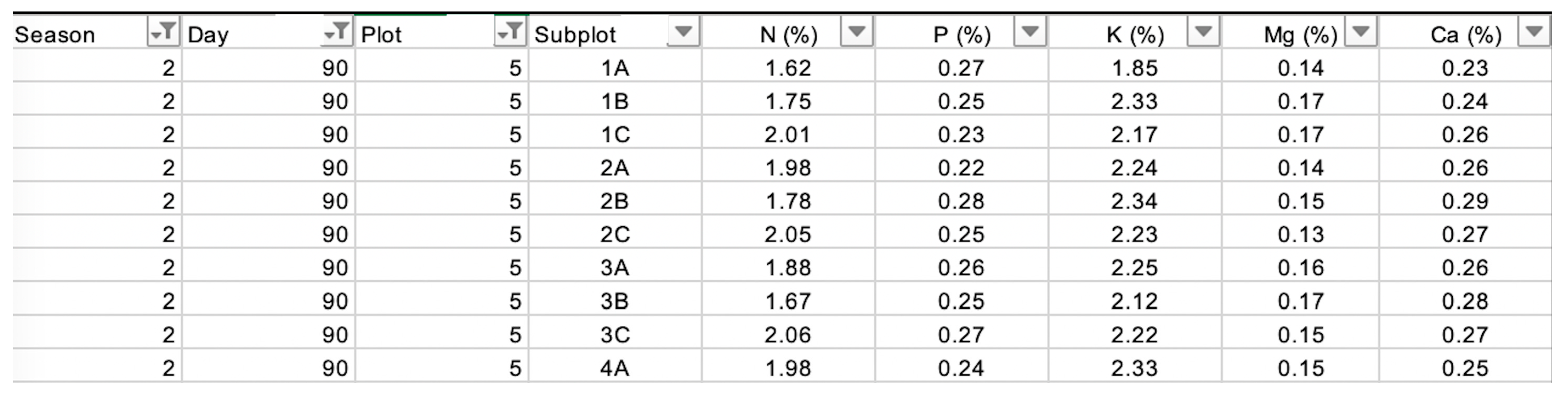
Missing Values	No

, comprising 348 observations and nine attributes. This multivariate dataset features a combination of categorical and numerical data, including spatiotemporal factors such as Season, Day, Plot, and Subplot.

The Season attribute categorizes data into two distinct seasons, denoted by the values 1 and 2, enabling the exploration of how seasonal changes influence rice nutrient levels, a fundamental aspect of rice production optimization. Additionally, the Day attribute, with three distinct values, 30, 60, and 90, introduces temporal granularity, facilitating an examination of nutrient content variations within each season. This temporal dimension is essential for understanding the influence of specific days on nutrient levels.

Furthermore, the Plot attribute categorizes data into four distinct plot locations represented by values 1, 3, 4, and 5, enabling the assessment of nutrient distribution across different areas within the study site, thus adding a spatial context to the analysis. Subplot further refines the spatial information by specifying 15 sublocations within each plot, denoted by values such as 1A, 1B, 1C, and so forth.

This fine-grained attribute is invaluable for scrutinizing nutrient variation within specific subregions of the plots, enhancing spatial precision. Additionally, the dataset incorporates nutrient concentration, composition, and co-existence (“N%”, “P%”, “K%”, “Mg%”, “Ca%”), which is vital for understanding rice growth and health. The dataset’s integrity is maintained, as it contains no missing values.

An example of the data content is shown in Figure 1, which shows the concentration of each nutrient based on the spatial information. The best range of the nutrients are N: [1.17, 2.47], P: [0.25, 0.3], K: [1.85, 2.52], Mg: [0.11, 0.17], and Ca: [0.23, 0.33], which has produced the maximum weight grain at the planting plot with range [29.26, 39.42] at the end of the planting cycle. These values are considered the best practice to guide the intervention plan for the user (farmer or scientist).

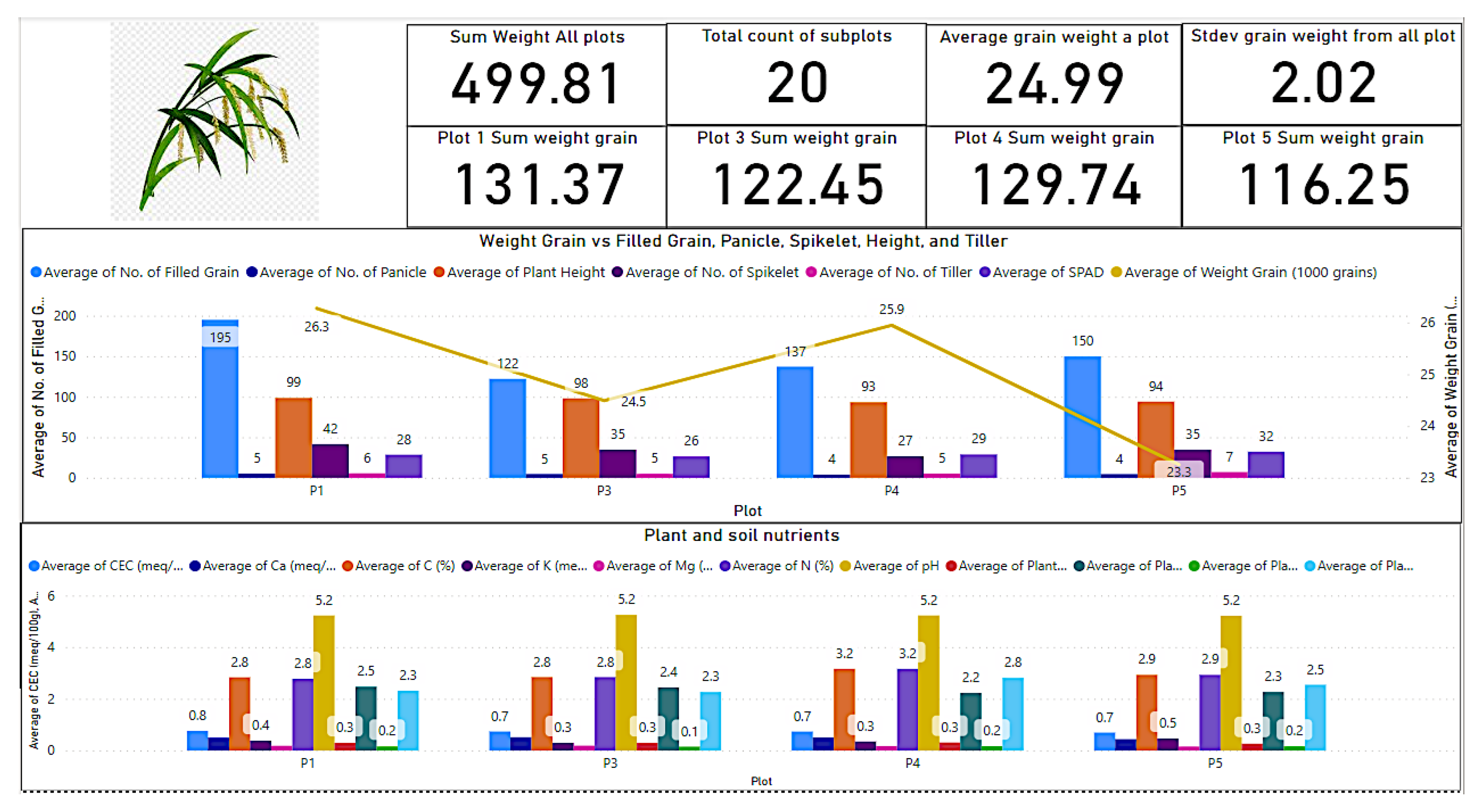
Figure 2 shows the dashboard that presents the average rice nutrient concentration across the growth period and the rice anatomical values at harvesting time, while Figure 3 shows the nutrient value distribution. From Figure 2, we can identify the relationship of the nutrient con-existence, composition, and concentration with the yield. The digital twin supports a three-staged insight for crop intelligence. First, we could also see the average values of nutrients that have led to the yield, and the nutrient values from the plant with the best yield become the benchmark.

So, this has motivated us towards the second intelligence by predicting the co-existence, concentration, and composition of the plant at each plot and subplot to know about their health. The third intelligence is nutrient recovery during the growth as an intervention mechanism, so that the predicted values can be a guide on precise additional nutrients to be added into the crop medium to optimize the yield. The precision of values for additional nutrients can mitigate unnecessary excess in fertilizer usage and waste pollution.

The nutrient concentration distribution, as depicted in

Table 3. Value distribution for the nutrients.

	N (%)	P (%)	K (%)	Mg (%)	Ca (%)
MIN	0.15	0.15	1.61	0.09	0.16
MAX	4.59	28.00	3.89	0.20	0.38
STDEV	0.77	1.48	0.45	0.02	0.04

, highlights the range of values for the key nutrients N (%), P (%), K (%), Mg (%), and Ca (%) that is essential for agricultural productivity. The minimum (MIN) and maximum (MAX) values illustrate the variability in nutrient levels, emphasizing the complexity of nutrient dynamics in agriculture. Standard deviation (STDEV) values quantify the degree of variability around the mean. This information is instrumental in precision agriculture, guiding targeted interventions based on specific nutrient needs. In the context of environmental sustainability, understanding these distributions enables our digital twin system to issue timely alerts and recommend nutrient recovery interventions when concentrations exceed recommended ranges. This proactive approach optimizes crop yield while minimizing the environmental impact associated with nutrient imbalances.

3.2. Data Pre-Processing Using Min–Max Normalization

Before visualization, the data exhibited variations in nutrient concentrations that prompted the need for exploration. The raw data contained outliers, which are data points significantly different from the majority of the observations. These outliers, if not addressed, can impact the understanding of the overall nutrient distribution and make it challenging to discern patterns and trends in the data.

The Min–Max normalization method is applied to rescale the input features between 0 and 1 during the pre-processing phase. This normalization technique is suitable for the prediction models of this study because it helps to ensure that all the input features are on the same scale and have the same range, which helps the linear regression models of this study converge faster and boost their performance. This approach removes noises from data and prevents the big scales from data by giving the range of [0, 1]. Equation (1) shows the formula of the Min–MAX method.

$$X_{Norm}=\frac{(X-X_{Min})}{(X_{Max}-X_{Min})}$$

(1)

where X is the original value of a data point, $X_{Min}$ is the minimum value in the dataset, $X_{Max}$ is the maximum value in the dataset, and $X_{Norm}$ is the normalized value of the data point. This formula ensures that the minimum value in the dataset is scaled to 0 and the maximum value is scaled to 1, with all other values falling between these two limits.

By applying a pre-processing method to the dataset, we can improve the stability and performance of the regression models. Once this stage is complete, we can proceed to the next stage, where we design a regression model based on the different variables in the dataset. This stage involves selecting an appropriate regression method and specifying the independent and dependent variables. Finally, we analyze the model and provide information on its performance and accuracy. 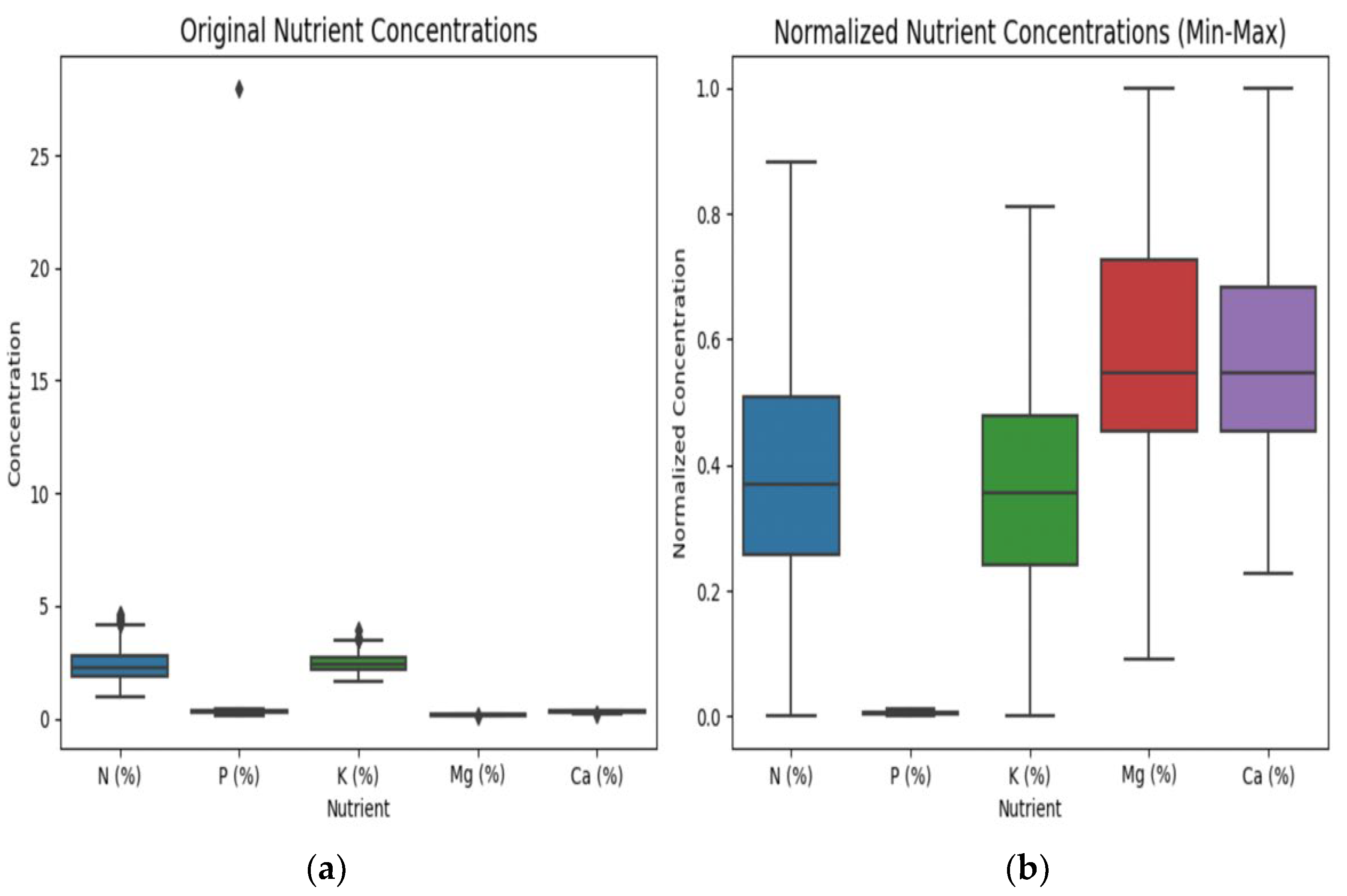Figure 3 illustrates the rice nutrients data before and after applying the Min–Max normalization method. The visual representation of the data highlights the impact of normalization on the distribution of nutrient concentrations.

The dataset under analysis consists of nutrient concentration data for rice samples, including attributes like nitrogen (N%), phosphorus (P%), potassium (K%), magnesium (Mg%), and calcium (Ca%). Prior to visualization, the data exhibited variations in nutrient concentrations that prompted the need for exploration. The raw data contained outliers, which are data points significantly different from the majority of the observations. These outliers, if not addressed, can impact the understanding of the overall nutrient distribution and make it challenging to discern patterns and trends in the data.

Therefore, to gain a deeper understanding of the nutrient concentration data and visualize its distribution, we employed box plots both before and after applying Min–Max normalization. The original box plots revealed the presence of outliers in the dataset, which was affecting the clarity of the distribution. To address this issue, Min-Max normalization was applied to scale the data. The box plots after normalization effectively showcased the distribution of nutrient concentrations without displaying outliers. This approach allows for a more accurate and informative representation of the data, aiding in the identification of central tendencies and variations while providing a clearer view of the data’s overall structure. The use of box plots before and after normalization aids in the assessment of data quality and the impact of data pre-processing techniques.

3.3. Nutrient Concentration and Composition Prediction

We present two approaches, namely, (i) single nutrient concentration prediction and (ii) nutrient composition concentration prediction, which are developed using EN, PN, SW, RR, LS, and LR algorithms. This section describes the development of the prediction models.

3.3.1. Single-Nutrient Concentration Prediction

We call the first approach single-nutrient concentration prediction, where five (5) models are developed based on different feature sets of the rice dataset, as shown in

Table 4. Single-nutrient concentration prediction setting.

Spatiotemporal Factors					Nutrients
Feature Set	Season	Day	Plot	Subplot	N (%)	P (%)	K (%)	Mg (%)	Ca (%)
FS1 (Ca%)	Y	Y	Y	Y	Y	Y	Y	Y	N
FS2 (Mg%)	Y	Y	Y	Y	Y	Y	Y	N	Y
FS3 (K%)	Y	Y	Y	Y	Y	Y	N	Y	Y
FS4 (P%)	Y	Y	Y	Y	Y	N	Y	Y	Y
FS5 (N%)	Y	Y	Y	Y	N	Y	Y	Y	Y

, by exploiting the nutrient concentration, co-existence, and composition. In Table 4, “Y” indicates that the spatiotemporal factors and nutrient features are used in the model building, while “N” indicates otherwise.

Referring to Table 4, the single-nutrient concentration setting has been constructed based on the selection of different features from spatiotemporal factors and nutrient features. These settings will be used for single-nutrient concentration prediction using six methods: EN, PN, SW, PR, LS, and LR.

Table 5. Parameter specification for six regression algorithms of EN, PN, SW, PR, LS, and LR in single-nutrient concentration and composition concentration prediction.

Model	Parameter	Values
EN	alpha	0.1
	L1_ratio	0.5
PN	degree	2
SW	Sequential Feature Selector	Automatically select features (no direct parameters involved)
PR	alpha	0.1
LS	alpha	0.1
LR	No additional parameters	---------

presents the parameter specifications applied to the six regression approaches of EN, PN, SW, PR, LS, and LR in single-nutrient concentration and composition concentration prediction.

Table 5 outlines the parameter specifications for six regression algorithms of EN, PN, SW, PR, LS, and LR in the context of predicting both single-nutrient concentration and composition concentration.

For EN, the parameters include an alpha value of 0.1 and an L1_ratio of 0.5. PN employs a degree of 2 for modeling. The SW automatically selects features without involving direct parameters. PR is characterized by an alpha value of 0.1, and LS also utilizes an alpha value of 0.1. LR, on the other hand, involves no additional parameters, as indicated by the dashed line in the “Values” column.

The steps for the single-nutrient concentration prediction are described in Algorithm 1, based on the parameters setting for the machine learning algorithms described in Table 5.

Algorithm 1: Single-nutrient concentration prediction

Input: Nutrient concentration dataset Process: Apply the Min-Max normalization method (Equation (1)) Set training ratio = 80% For each feature set, fs in Table 4: FS1,…, FS5 Load FSx to be the predictors ModelENx = Develop Elastic Net regression using FSx with parameters in Table 5 ModelSWx = Develop Polynomial regression using FSx with parameters in Table 5 ModelSWx = Develop Stepwise regression using FSx with parameters in Table 5 ModelRRx = Develop Ridge regression using FSx with parameters in Table 5 ModelLSx = Develop Lasso regression using FSx with parameters in Table 5 ModelLRx = Develop Linear regression using FSx with parameters in Table 5 End For Output: ModelENCa, ModelENMg, ModelENK, ModelENP, ModelENN, ModelPNCa, ModelPNMg, ModelPNK, ModelPNP, ModelPNN, ModelSWCa, ModelSWMg, ModelSWK, ModelSWP, ModelSWN, ModelSWCa, ModelSWMg, ModelSWK, ModelSWP, ModelSWN, ModelRRCa, ModelRRMg, ModelRRK, ModelRRP, ModelRRN, ModelLSCa, ModelLSMg, ModelLSK, ModelLSP, ModelLSN, ModelLRCa, ModelLRMg, ModelLRK, ModelLRP, ModelLRN.

In relation to Algorithm 1, the process for single-nutrient concentration prediction, outlined in Algorithm 1, involves applying Min-Max normalization to the nutrient concentration dataset and setting an 80% training ratio. For each of the five feature sets (FS1 to FS5) detailed in Table 3, the algorithm loads the respective features and employs six regression models (Elastic Net, Polynomial, Stepwise, Ridge, Lasso, Linear), each with its parameters specified in Table 4. The result is a set of trained models for predicting nutrient concentrations (Ca, Mg, K, P, N) denoted by prefixes such as ModelEN_Ca, ModelEN_Mg, and so on. The models are developed using various regression techniques tailored to each feature set, creating a comprehensive framework for nutrient concentration prediction.

3.3.2. Nutrient Composition Concentration Prediction

In the second approach, a model is developed based on different feature sets of the rice dataset, as shown in

Table 6. Nutrient composition concentration prediction setting.

Spatiotemporal Factors					Nutrients
Feature Set	Season	Day	Plot	Subplot	N (%)	P (%)	K (%)	Mg (%)	Ca (%)
FS6 (All)	Y	Y	Y	Y	N	N	N	N	N

, based on solely the spatiotemporal factors.

Referring to Table 6, the nutrient composition concentration prediction setting has been constructed by incorporating features from both spatiotemporal factors and nutrient features.

These settings will be utilized for nutrient composition concentration prediction using six methods: EN, PN, SW, PR, LS, and LR. The parameter specifications for these models in nutrient composition concentration prediction are consistent with those applied for single-nutrient concentration prediction (refer to Table 5).

The steps outlined in Algorithm 2 illustrate the processes for nutrient composition concentration prediction, developed based on the similar parameter specifications listed in Table 4 for single-nutrient concentration prediction.

Algorithm 2: Nutrient composition concentration prediction

Input: Nutrient concentration dataset Process:  1. Apply the Min-Max normalization method (Equation (1))  2. Set training ratio = 80%  3. Load FS6 from Table 6  4. ModelENx = Develop Elastic Net regression using FSx with parameters in Table 5  5. ModelSWx = Develop Polynomial regression using FSx with parameters in Table 5  6. ModelSWx = Develop Stepwise regression using FSx with parameters in Table 5  7. ModelRRx = Develop Ridge regression using FSx with parameters in Table 5  8. ModelLSx = Develop Lasso regression using FSx with parameters in Table 5  9. ModelLRx = Develop Linear regression using FSx with parameters in Table 5

Output: ModelENAll, ModelPNAll, ModelSWAll, ModelRRAll, ModelLSAll, ModelLRAll

Algorithm 2, designed for nutrient composition concentration prediction, starts by normalizing the input nutrient concentration dataset using the Min–Max method and setting an 80% training ratio. It then exclusively utilizes features from FS6 in Table 6 to develop six regression models—Elastic Net, Polynomial, Stepwise, Ridge, Lasso, and Linear—each configured with parameters specified in Table 5. The resulting output comprises comprehensive models denoted as ModelEN_All, ModelPN_All, ModelSW_All, ModelRR_All, ModelLS_All, and ModelLR_All. This algorithm provides an efficient means of predicting nutrient composition concentrations based on the designated features and regression techniques.

4. Experimental Setting

This section presents the experimental results for Elastic Net Regression, Polynomial Regression, Stepwise Regression, Ridge Regression, Lasso Regression, and Linear Regression to predict rice nutrient levels using FS one until six. Table 4 and Figure 4 display the RMSE scores of all six models, where Polynomial Regression has the best performance in four models to predict Ca%, K%, P%, and N%, with an average of 0.1502 RMSE, except in Model 2 (prediction of Mg%), with very little standard deviation (0.1980).

4.1. The Performance of the Single-Nutrient Concentration Approach

We present

Table 7. Performances of Ca prediction using approach 1.

Algorithm	R2 Score	MAE	RMSE
ModelENCa	0.0	0.0297	0.0362
ModelPNCa	0.5017	0.0204	0.0255
ModelESWCa	0.0257	0.0292	0.0357
ModelRRCa	0.0869	0.0281	0.0345
ModelLSCa	0.0	0.0361	0.0297
ModelLRCa	0.0931	0.0279	0.0345
AVG	0.1179	0.0286	0.0327
STDEV	0.1942	0.0050	0.0042

,

Table 8. Performance of Mg prediction using approach 1.

Algorithm	R2 Score	MAE	RMSE
ModelENMg	0.0	0.0154	0.0193
ModelPNMg	−3.1900	0.0301	0.0395
ModelESWMg	0.0879	0.0151	0.0184
ModelRRMg	0.1734	0.0142	0.0176
ModelLSMg	0.0	0.0154	0.01934
ModelLRMg	0.1742	0.0141	0.0175
AVG	−0.451	0.0174	0.0219
STDEV	1.3401	0.0063	0.0086

,

Table 9. Performance of K prediction using approach 1.

Algorithm	R2 Score	MAE	RMSE
ModelENK	0.1967	0.3101	0.3991
ModelPNK	0.8496	0.1275	0.1726
ModelESWK	0.0926	0.3464	0.4241
ModelRRK	0.5873	0.2266	0.2860
ModelLSK	0.1391	0.3235	0.4131
ModelLRK	0.5895	0.2261	0.2852
AVG	0.4091	0.2600	0.3300
STDEV	0.3087	0.0823	0.0993

,

Table 10. Performance of P prediction using approach 1.

Algorithm	R2 Score	MAE	RMSE
ModelENP	0.0	0.0529	0.0651
ModelPNP	0.8308	0.0212	0.0267
ModelESWP	0.4180	0.0377	0.0497
ModelRRP	0.6193	0.0311	0.0402
ModelLSP	0.0	0.0529	0.0651
ModelLRP	0.6202	0.0312	0.040
AVG	0.4147	0.0378	0.0478
STDEV	0.3468	0.0128	0.0153

and

Table 11. Performance of N prediction using approach 1.

Algorithm	R2 Score	MAE	RMSE
ModelENN	0.3006	0.4524	0.6326
ModelPNN	0.5862	0.3808	0.4866
ModelESWN	0.4240	0.4388	0.5741
ModelRRN	0.5508	0.3657	0.5070
ModelLSN	0.1994	0.4948	0.6768
ModelLRN	0.5532	0.3661	0.5056
AVG	0.4357	0.4164	0.5638
STDEV	0.1574	0.0535	0.0777

to explain the performance of the single-nutrient concentration approach by using R², MAE, and RMSE. A larger R² value is generally considered better. An R² value closer to one suggests that a larger proportion of the variation in the dependent variable is accounted for by the independent variables in the model, indicating a better fit. However, it is important to note that a high R² does not necessarily imply causation or the absence of model errors, and other factors should be considered in evaluating the overall validity of the regression model. MAE represents the average absolute difference between the predicted values and the actual values. The smaller the MAE, the better the model performance. MAE is less sensitive to outliers compared to RMSE. Lower values of MAE and RMSE indicate better model performance.

According to Table 7, the optimal model for predicting Ca is ModelPN_Ca, demonstrating consistent performance across all evaluation metrics of R² Score, MAE, and RMSE. The bold highlighting in Table 7 indicates the significantly superior performance of the PN algorithm compared to other algorithms, emphasizing its effectiveness in capturing the variability of nutrient values. Two algorithms, EN and LS, could not capture the variability in the dataset for predicting Ca, based on the zero R² value.

Contrary to its performance in Table 7, the PN algorithm shows a bad performance for magnesium. The best for magnesium prediction is the LR algorithm. The negative R² value of PN implies that the model is so inadequate that it is worse than a naive model that merely predicts the mean of the dependent variable for all observations. This indicates that PN could have been overfit and too complex for the given data, and it fits noise rather than the underlying patterns.

The performances of LR and RR are very similar, which reflects their high similarity. Both algorithms assume a linear relationship between the independent variables and the dependent variable. The models are expressed as linear combinations of the input features. Both methods aim to minimize a certain objective function to find the optimal set of coefficients that best fits the data. In LR, this is typically done by minimizing the sum of the squared differences between the predicted and actual values. In RR, the objective function includes an additional regularization term.

The primary difference between RR and LR lies in how they handle multicollinearity and overfitting. RR uses regularization terms and penalizes large coefficients, helping to mitigate the effects of multicollinearity and prevent overfitting. The regularization term is controlled by a hyperparameter (usually denoted as “alpha” or “lambda”). LR does not include a regularization term in the objective function. It is more prone to overfitting when dealing with highly correlated features (multicollinearity) or when the number of features is close to or exceeds the number of observations.

PN maintains the best algorithm for K prediction, and, again, the performances of RR and LR are very similar for predicting K. As explained, RR is a modified version of LR that adds a regularization term to address certain issues, particularly multicollinearity. If the correlation between independent variables is high, RR can provide more stable and reliable coefficient estimates compared to LR. Since the performance of RR is better in predicting K, this indicates that the dataset for the training possesses multicollinearity.

Likewise, the best technique for P prediction is PN, and it is observed that the performance of PN in this nutrient prediction is the best compared to other nutrients. All the other algorithms also had better scores, which indicates that the values in the features used for training the P prediction are more homogeneous compared to the earlier models.

Similarly, PN achieved the best performance in comparison with the other models. All models had lower performances in predicting N compared to predicting P. It is also observed that the performance of SW in predicting N is similar to that predicting P, when compared against RR and LR. Although LR and RR show stability and generalizability across different datasets, SW has better performance in this nutrient compared to Ca and Mg because of its simplicity drawback and tendency to assume that the relationship between variables is best represented by a combination of selected features.

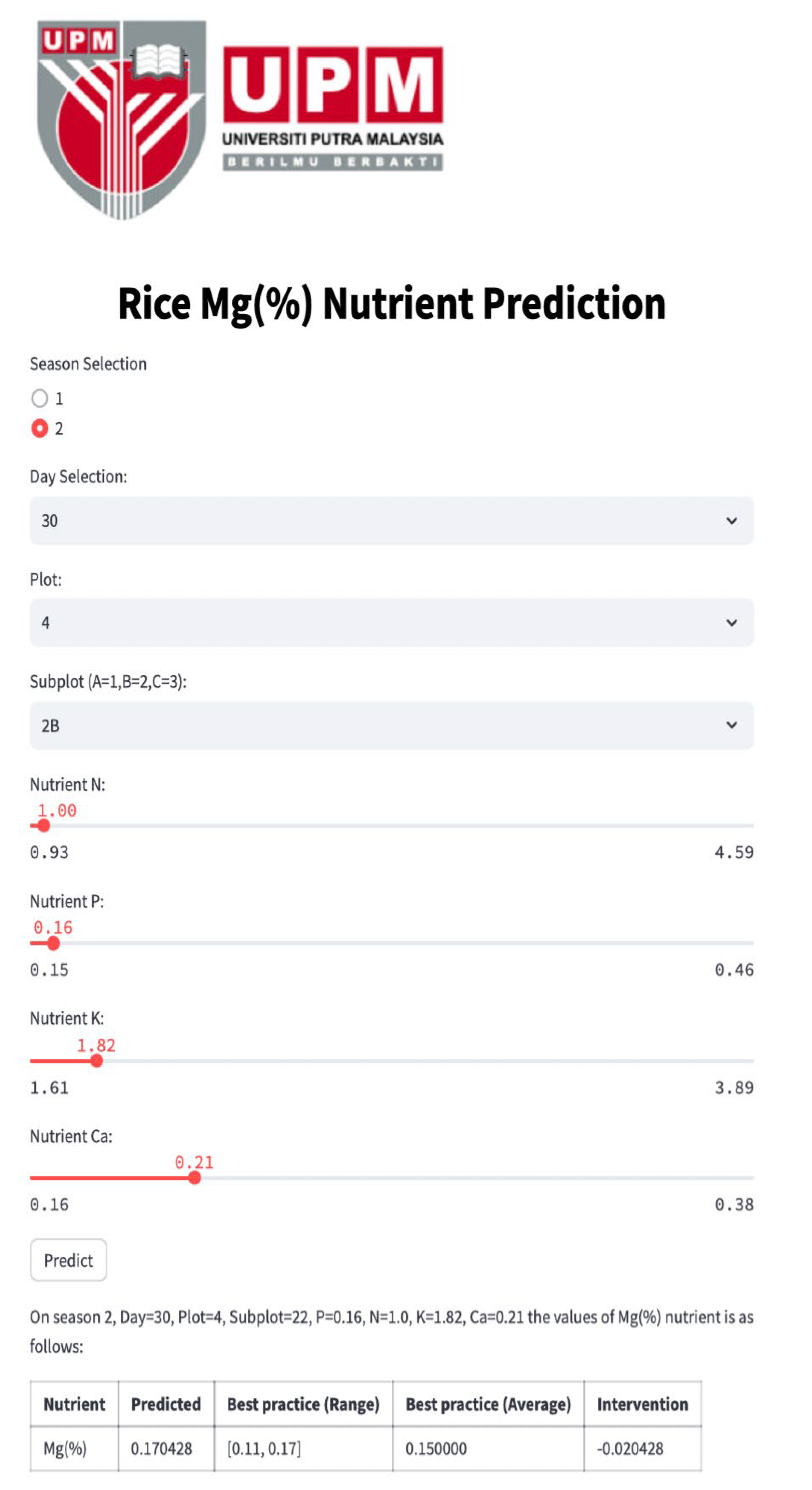
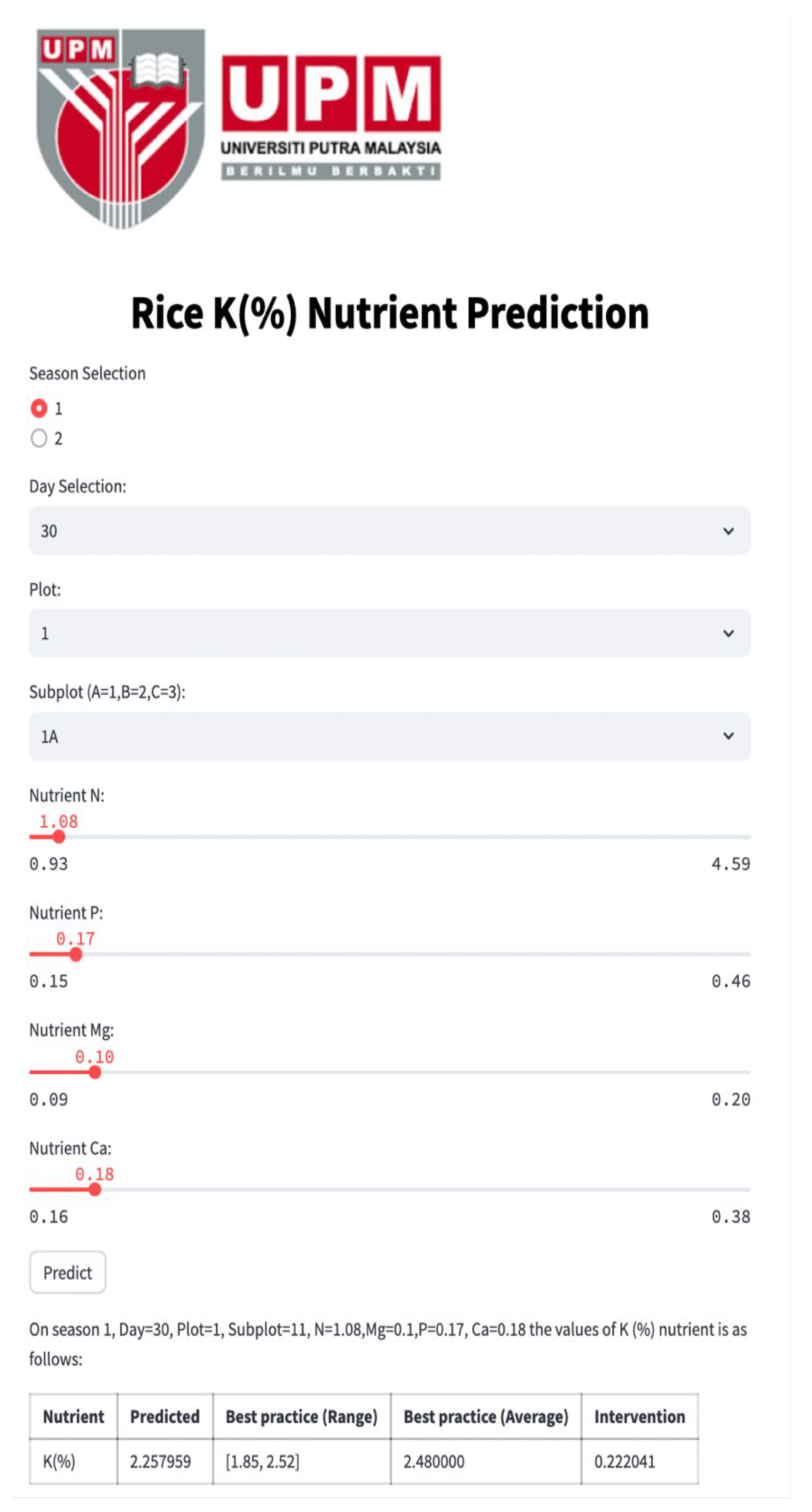
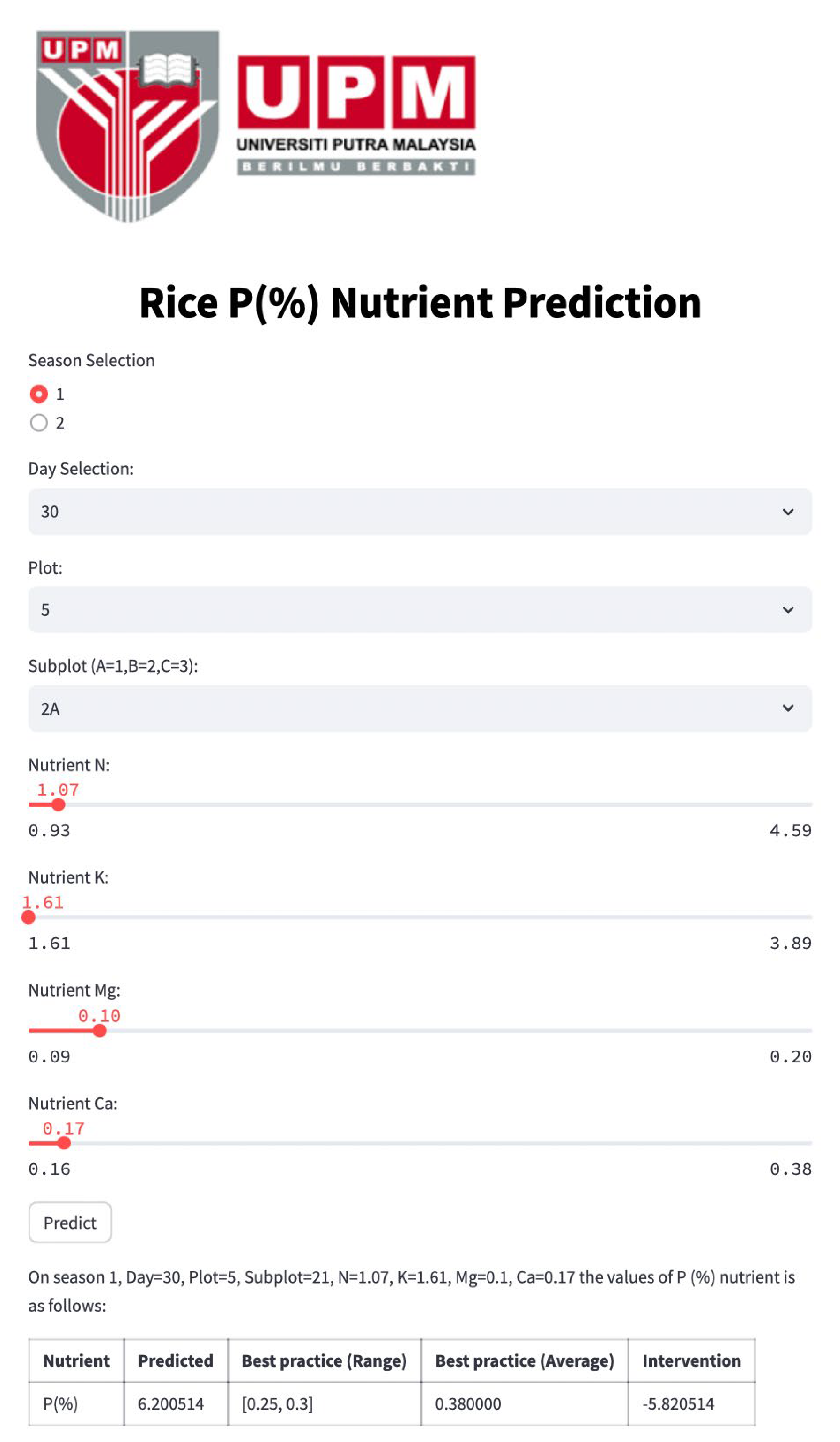
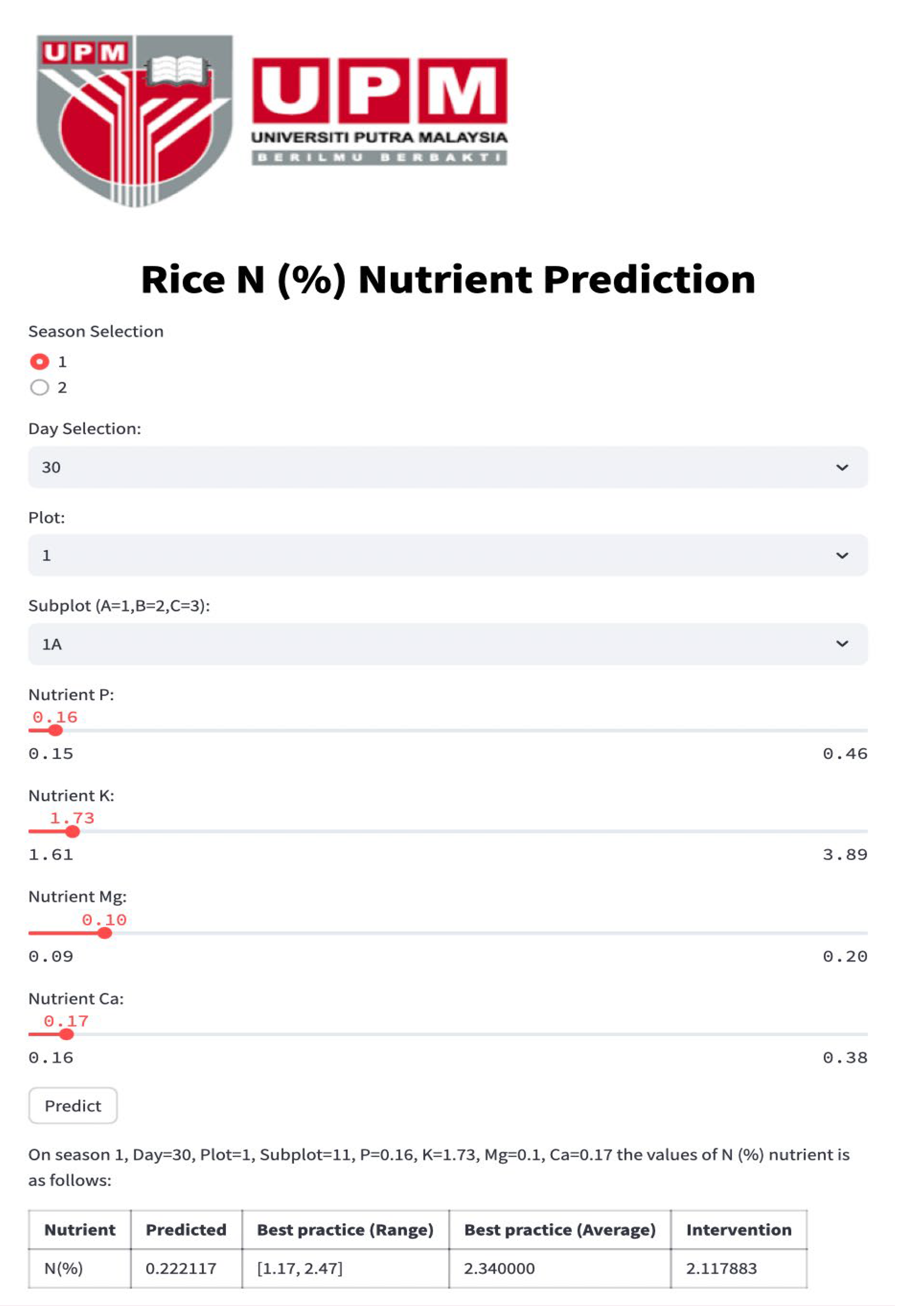
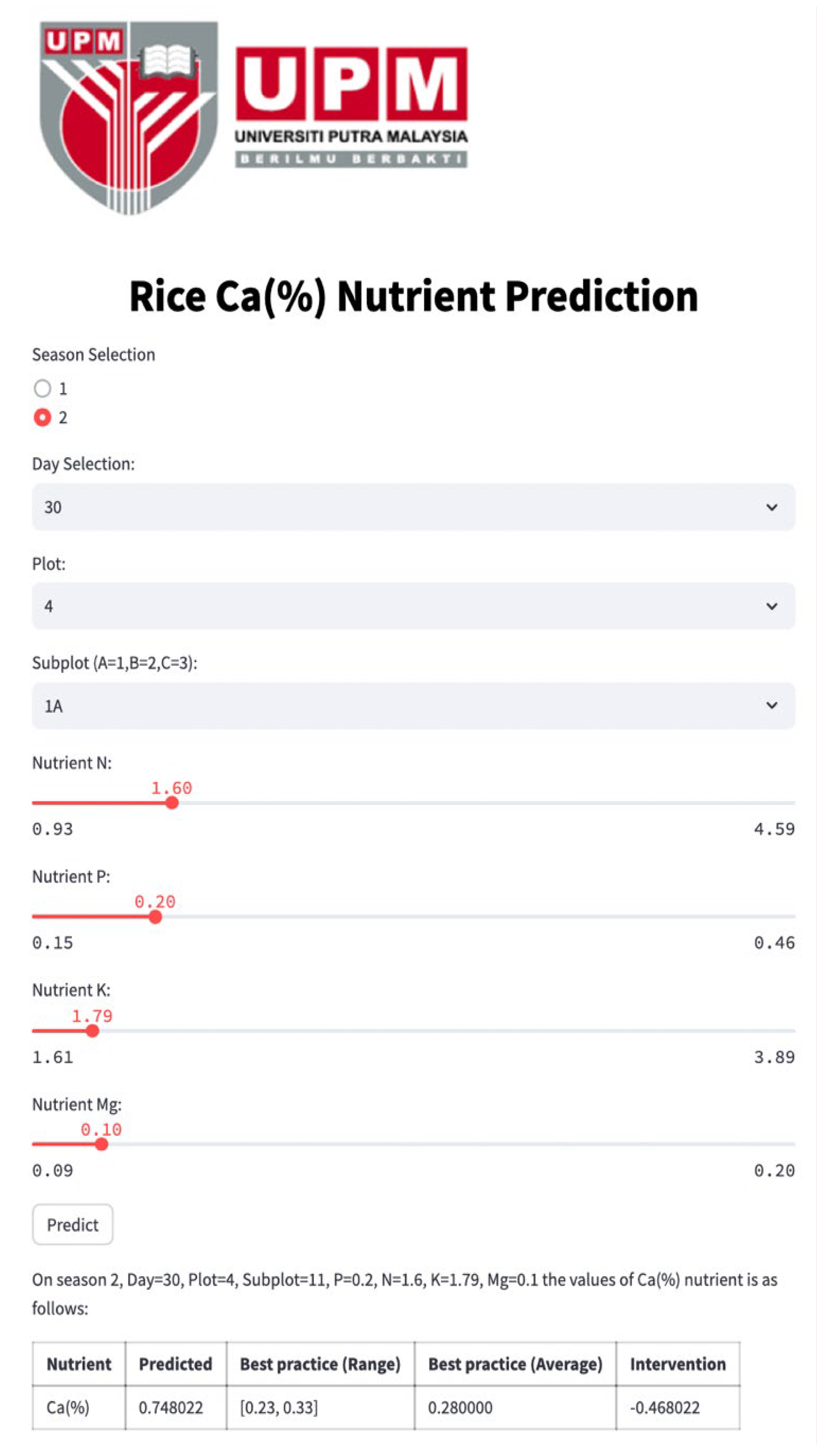
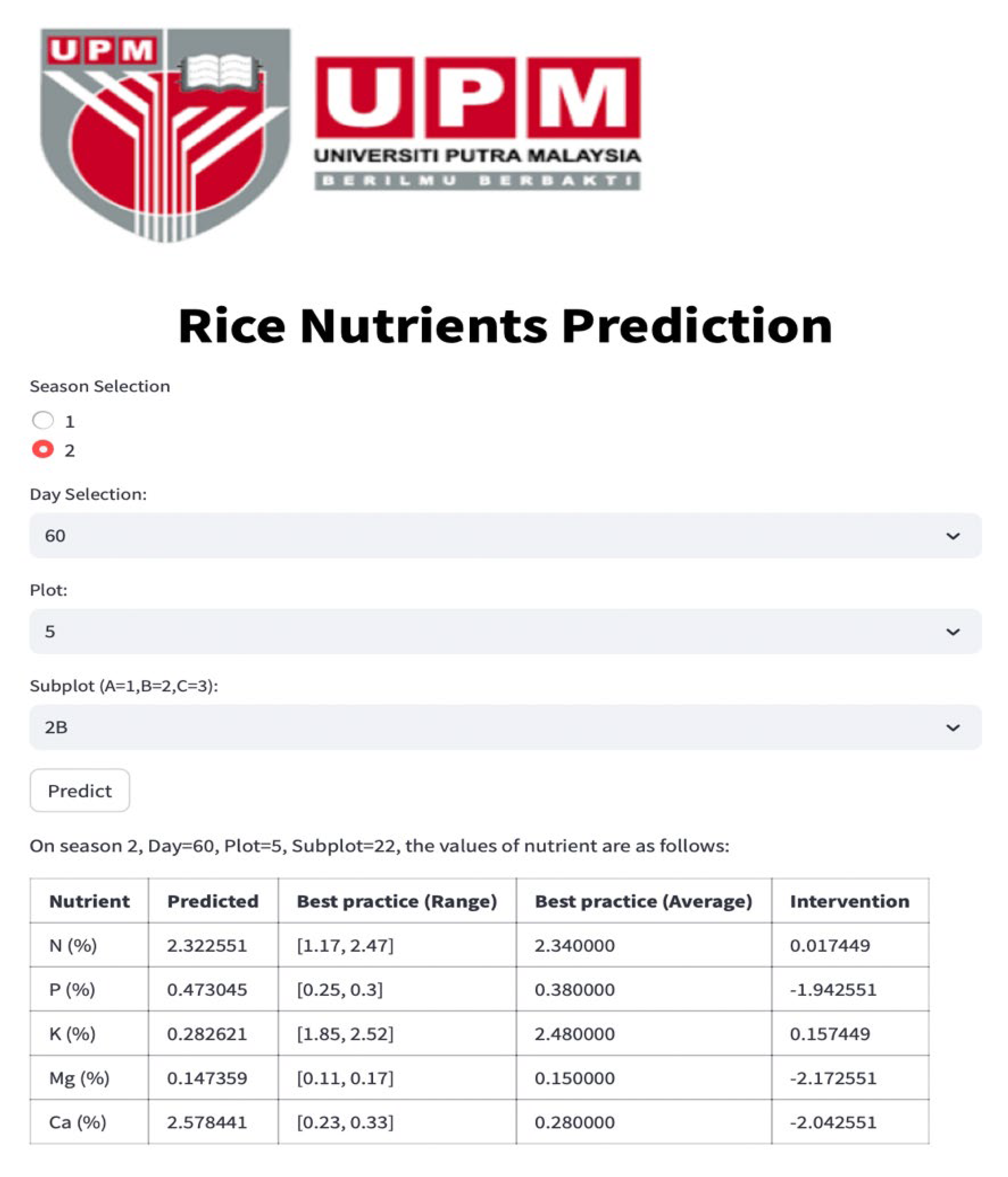
Figure 4, Figure 5, Figure 6, Figure 7 and Figure 8 depict the Streamlit outputs for the single-nutrient prediction of Ca, Mg, K, P, and N, respectively, based on the best-performing model, PN. The predicted values for each nutrient are computed utilizing the PN model, taking into account spatial–temporal parameters and other relevant nutrient inputs. The diagrams illustrate that the predicted nutrient concentrations are used to recommend the amount of nutrient recovery, by comparing them against the benchmark nutrient values.

Figure 4. Rice Ca nutrient prediction based on other nutrients of N, P, K, and Mg.

Figure 4. Rice Ca nutrient prediction based on other nutrients of N, P, K, and Mg.

Referring to the aforementioned Streamlit interface for individual nutrients, including Ca, Mg, K, P, and N, the application provides essential values for “predicted”, “Best practice (Range)”, “Best practice (Average)”, and “Intervention.” The predicted values for each nutrient are computed utilizing the PN model, taking into account spatial–temporal parameters and other relevant nutrient inputs.

The “Best practice Range” and “Best practice Average” values specify the optimal ranges and averages of nutrient concentrations, offering valuable benchmarks for nutrient levels. To further enhance precision in nutrient management, the intervention value is calculated by estimating the difference between the best practice average and the predicted value derived from the PN model. This intervention value serves as a critical metric for nutrient recovery interventions, providing insights into the precise amount of nutrients required for optimal crop growth.

Therefore, in the context of precision agriculture and environmental sustainability, the crafted Streamlit tool for predicting individual nutrients, utilizing prior knowledge of other nutrient concentrations, offers advantages to farmers and scientists seeking specific insights into individual nutrient levels. This method proves especially advantageous when a sensor dedicated to a specific nutrient experiences a malfunction. As a result, our digital twin system promptly alerts users about sensor malfunctions and supplies predictive values while waiting for sensor replacement. This immediate functionality guarantees continuous monitoring, safeguarding data accuracy and ensuring the effectiveness of precision agriculture practices.

4.2. The Performance of the Nutrient Composition Concentration Approach

ModelPN_All appears to be the best-performing model based on R², MAE, and RMSE. It explains a significant proportion of variability and provides accurate predictions. ModelRR_All and ModelLR_All have the same R², MAE, and RMSE values, indicating similar performance. They both exhibit a moderate level of explained variability and reasonable predictive accuracy. ModelEN_All, ModelESW_All, and ModelLS_All have lower R² values, suggesting limited ability to explain variability. They also have higher MAE and RMSE values, indicating higher prediction errors compared to the better-performing models. The choice of features included in the models can significantly impact performance. Models that incorporate irrelevant or highly correlated features may exhibit lower accuracy. The results (

Table 12. Performance of approach 2 to predict all nutrients.

Algorithm	R2 Score	MAE	RMSE
ModelENAll	0.0771	0.1814	0.2376
ModelPNAll	0.5237	0.1211	0.1502
ModelESWAll	0.0450	0.2054	0.2572
ModelRRAll	0.3066	0.1477	0.1949
ModelLSAll	0.0377	0.1918	0.2494
ModelLRAll	0.3066	0.1477	0.1949
AVG	0.2161	0.1659	0.2140
STDEV	0.1957	0.0321	0.0412

) also indicate that the features incorporated have a complex relationship with each other and the target variable.

The experiment results led us to the conclusion that regression models have good performance in informing nutrient co-existence, concentration, and composition. This insight allows interventions to increase nutrient recovery to optimize the crop’s yield. PN generally outperformed the other tested algorithms in terms of producing higher R² values and lower MAE and RMSE values for almost all models. This is due to the ability of the polynomial function to capture nonlinear relationships among variables. However, it should be noted that for Mg, the Polynomial Regression algorithm produced a negative R² value, indicating that it explained less variance in the dependent variable than a horizontal line. Therefore, the polynomial function was not well suited for predicting nutrient content in Mg. In contrast, LR produced better performance compared to the other methods for Mg, signifying that this model was better approximated by a straight-line relationship. This finding highlights the significance of considering the specific nature of the data and the relationships between variables when selecting the most appropriate regression model for nutrient prediction.

Figure 9 illustrates the Streamlit outputs for the prediction of nutrient composition concentrations, based on the best-performing model, PN.

Referring to the Figure 9 interface for nutrient composition concentrations, similar to the single-nutrient prediction (see Figure 4, Figure 5, Figure 6, Figure 7 and Figure 8), the application furnishes crucial values for “predicted”, “Best practice (Range)”, “Best practice (Average)” and “Intervention”. The predicted values for each nutrient are calculated employing the PN model, considering spatial–temporal parameters and other pertinent nutrient inputs.

The “Best practice Range” and “Best practice Average” values delineate the optimum range and averages of nutrient concentrations, providing valuable benchmarks for nutrient levels. Furthermore, this information serves as a comprehensive intervention preparation tool by informing farmers or scientists about the anticipated nutrient concentration. The projected value, in turn, facilitates the digital twin system in suggesting the appropriate amount of nutrient recovery, aligning with established best practices.

So, the provided streamlit for rice nutrient’s composition concentrations’ prediction serves as a powerful intervention preparation tool. By informing farmers and scientists about the anticipated nutrient concentrations, this approach enables the digital twin system to suggest the precise amount of nutrient recovery aligned with best practices. This proactive and informed approach not only optimizes crop yields but also minimizes the environmental footprint associated with excessive fertilizer application.

4.3. RMSE Analysis and Approach Performance Highlights

To identify the best model, we provide an analysis of RMSE across both approaches.

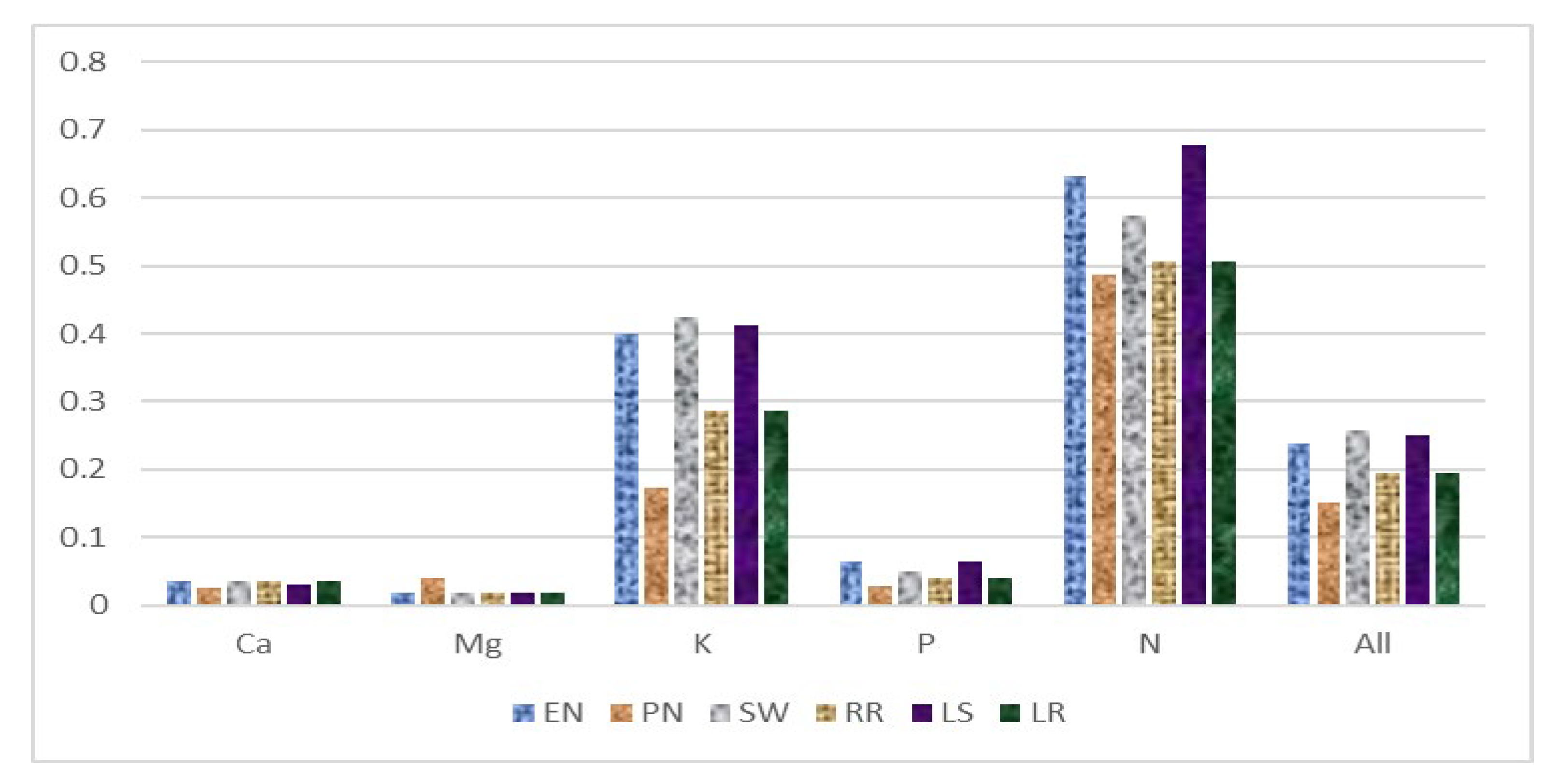
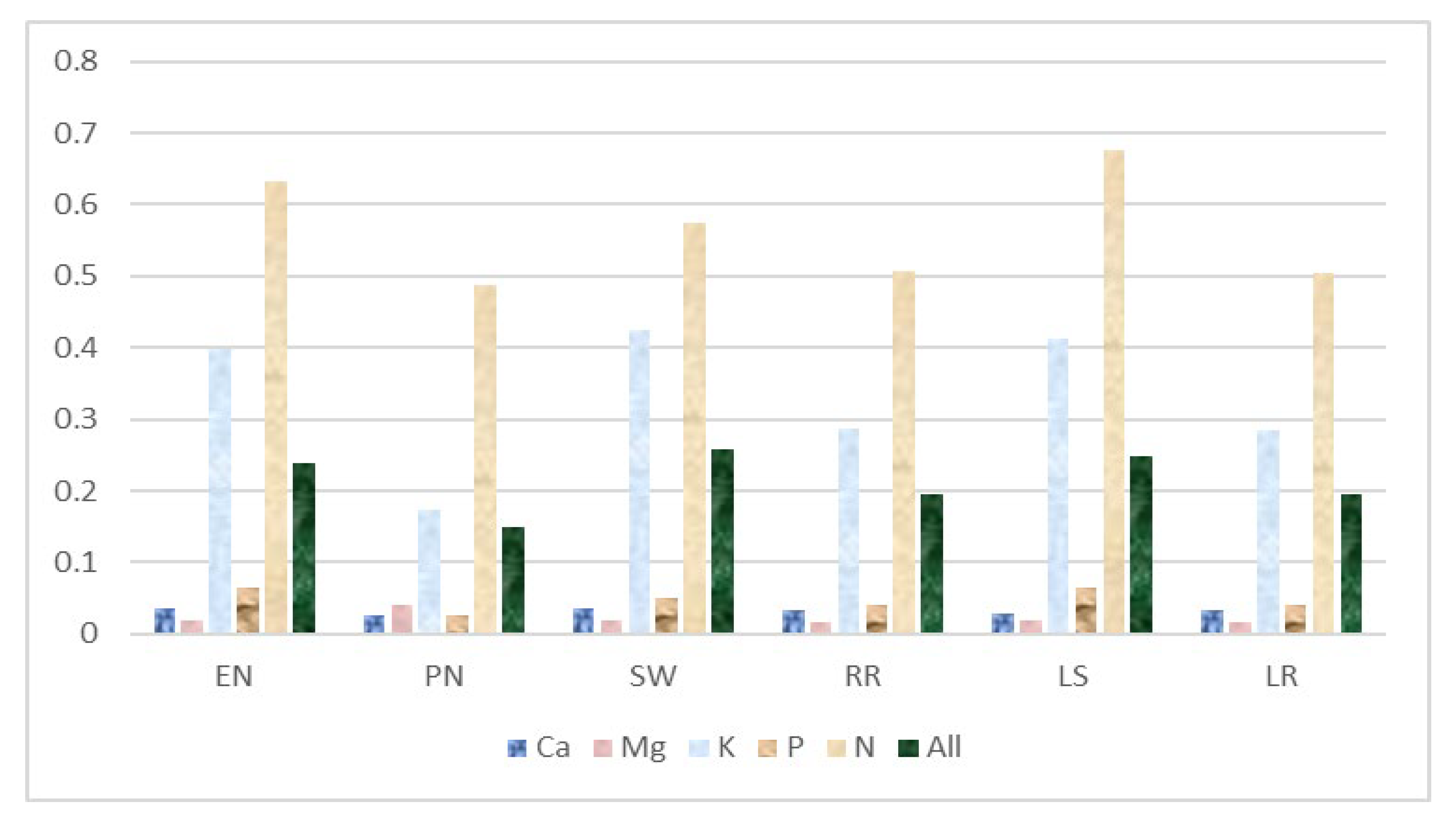
The best performance of an algorithm for FS2 is Linear Regression. In terms of the performance of predicting each nutrient, FS2 is the easiest to be predicted, based on the average (AVG) of RMSE for this model, at 0.0219 (Figure 10). On the contrary, according to Figure 11, the percentage of N is the most difficult and inconsistent performance across the regression models, with an average of RMSE at 0.5638.

Table 13. RMSE with averages and STDEV.

Method	Ca	Mg	K	P	N	All	AVG	STDEV
EN	0.0362	0.0193	0.3991	0.0651	0.6326	0.2376	0.2305	0.2738
PN	0.0255	0.0395	0.1726	0.0267	0.4866	0.1502	0.1502	0.1979
SW	0.0357	0.0184	0.4241	0.0497	0.5741	0.2572	0.2204	0.2601
RR	0.0345	0.0176	0.2860	0.0402	0.5070	0.1949	0.1771	0.2152
LS	0.0297	0.0193	0.4131	0.0651	0.6768	0.2494	0.2408	0.2934
LR	0.0345	0.0175	0.2852	0.0400	0.5056	0.1949	0.1766	0.2146
AVG	0.0327	0.0219	0.3300	0.0478	0.5638	0.2140
STDEV	0.0042	0.0086	0.0993	0.0153	0.0777	0.0412

presents the Root Mean Square Error (RMSE) along with average and standard deviation (STDEV) values for six Linear Regression algorithms.

4.4. Statistical Analysis

For this investigation, this study chose to use parametric statistical analysis because the assumptions of normality and equal variance are likely to be met given the data and the fact that we are comparing means within each regression model. Additionally, parametric tests are generally more powerful than non-parametric tests, meaning they have a greater ability to detect differences between groups when they exist.

The normality assumption was evaluated through the Shapiro–Wilk test, which is a commonly used test for normality. This test checks whether the data follows a normal distribution. The equal variance assumption was examined using Levene’s test. The Shapiro–Wilk test for normality was applied to the residuals of the regression models, and the results indicated that the residuals were normally distributed (p-value > 0.05). Additionally, Levene’s test was employed to assess the equality of variances among the groups, and the results did not suggest any significant deviation from homogeneity of variances (p-value > 0.05).

The application of these tests supports the validity of the ANOVA results presented in

Table 14. ANOVA test for performance analysis.

Anova: Single Factor
SUMMARY
Groups		Count	Sum	Average	Variance
FS1		6	0.1961	0.0327	1.77137 × 10−5
FS2		6	0.13164	0.0219	7.46328 × 10−5
FS3		6	1.9801	0.3300	0.0098
FS4		6	0.2868	0.0478	0.0002
FS5		6	3.3827	0.5638	0.0060
FS6		6	1.2842	0.2140	0.0017
ANOVA
Source of Variation	SS	df	MS	F	p-value
Between Groups	1.394	5	0.2787	93.3932	2.3253 × 10−17
Within Groups	0.0895	30	0.0030
Total	1.4833	35

. These tests, along with the reported F-statistics and p-values, confirm that the assumptions necessary for ANOVA were satisfied. Therefore, we can observe differences among the six designed regression models that are statistically significant and not a result of violations of normality or equal variance assumptions. Table 14 presents the ANOVA test for six designed regression models using different regression methods of “Elastic Net Regression”, “Polynomial regression”, “Stepwise regression”, “Ridge regression”, “Lasso regression” and “Linear Regression”.

Based on the ANOVA test with a p-value of 2.3253 × 10⁻¹⁷ and an alpha level of 0.05, we can conclude that there is a statistically significant difference among the six designed regression models. Therefore, we reject the null hypothesis that there is no significant difference and accept the alternative hypothesis that at least one of the regression models has a different performance value than the others.

Post hoc analysis was conducted using the Tukey Honestly Significant Difference (Tukey HSD) test to determine specific pairwise differences between the regression models. This test accounts for multiple comparisons and provides valuable insights into which models significantly differ in performance.

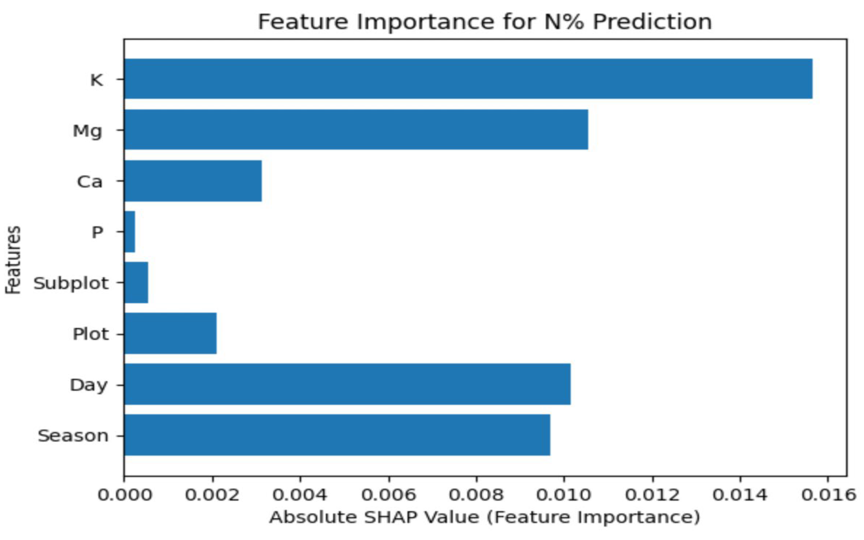
Based on the results of the ANOVA test, Model 5 demonstrated better performance compared to other designed feature set models (refer to Table 4). As a result, to gain insight into the impact of each nutrient on N% nutrient concentration, we utilized SHAP visualization. Figure 12 illustrates the effect of each nutrient on N% nutrient concentration.

Referring to Figure 12, the attributes K (potassium), Mg (magnesium), Day, Season, Ca (calcium), Plot, SubPlot, and P (phosphorus) appear to have varying levels of impact on N% nutrient concentration. Potassium (K) has the highest impact, followed by magnesium (Mg), indicating that their concentrations in the soil or nutrient supply significantly influence N%. The day and season when measurements are taken also play essential roles, while attributes like calcium (Ca), Plot, SubPlot, and phosphorus (P) have varying degrees of influence, with P showing the lowest impact. Therefore, this visualization can be valuable for optimizing agricultural and environmental practices to manage nutrient levels effectively, considering specific local conditions and domain knowledge.

5. Conclusions and Future Work

The crop digital twin offers a revolution to monitor and intervene in crop health management. The physical twin surveils the condition of the crop, and this information can be analyzed by the digital twin to provide suggestions for countermeasures, such as nutrient enrichment to increase concentration levels.

Predicting nutrient levels is crucial for optimizing fertilizer usage and ensuring a balanced nutrient supply, leading to higher-quality and increased yields, and reduced environmental impact. The importance of accurately anticipating essential nutrients, such as nitrogen (N), phosphorus (P), potassium (K), calcium (Ca), and magnesium (Mg), in rice cannot be overstated, as it directly impacts crop yield, quality, and environmental sustainability. The challenges in this field stem from the complexities introduced by the variability in nutrient content, the diversity of analytical approaches, data availability constraints, genetic diversity, and the associated costs and time investments.

To address these challenges, this research has presented two approaches, namely, (i) single-nutrient concentration prediction and (ii) nutrient composition concentration prediction, to explore a range of regression algorithms, including Elastic Net Regression, Polynomial Regression, Stepwise Regression, Ridge Regression, Lasso Regression, and Linear Regression, to predict rice nutrient content. These algorithms have proven to be invaluable tools for capturing both linear and nonlinear correlations among various nutrients, offering a structured, data-driven approach to understanding and managing the complexities of rice nutrition.

The findings reveal that the Polynomial Regression algorithm consistently outperforms the other models for predicting several nutrients, particularly calcium (Ca%), potassium (K%), phosphorus (P%), and nitrogen (N%). This algorithm’s ability to handle both small and large datasets, along with its proficiency in capturing nonlinear relationships, makes it a favorable choice for optimizing nutrient management practices. It is important to note, however, that Model 2, focused on predicting magnesium (Mg%), demonstrated a unique characteristic, as Linear Regression outperformed Polynomial Regression.

The dashboard in the digital twin visualizes the current nutrient content of the crop as a surveillance mechanism, while the predicted nutrient concentration is a valuable insight for precise fertilization to be added for nutrient recovery. This may mitigate fertilization overload and waste pollution. Although, this research currently addresses manual intervention, the implementation of the regression method supports the development of a low-resourced crop digital twin, enabling fast computations.

In summary, these regression models provide essential insights into rice nutrient prediction, offering a pathway to optimize fertilizer use, ensure balanced nutrient supply, enhance rice quality, and reduce environmental impact. They contribute to the development of standardized methodologies for nutrient prediction and promote more sustainable and environmentally friendly rice cultivation practices. The choice of the most suitable regression model depends on the specific characteristics of the dataset and the nature of the nutrient interactions. Therefore, the selection of the appropriate algorithm is pivotal to achieving the highest predictive accuracy for rice nutrient content.