Bi-Objective Function Optimization for Welding Robot Parameters to Improve Manipulability

Abstract

This paper presents a study on optimal design to determine the installation position and link lengths of a robot within a designated workspace for welding, aiming to minimize singularities during the robot’s motion. Bi-objective functions are formulated to minimize singularities while maximizing the volumes of linear velocity manipulability ellipsoid and angular velocity manipulability ellipsoid, respectively, ensuring isotropy. We have constructed a simulation environment incorporating PID control to account for robot tracking errors. This environment was utilized as a simulator to derive a Bi-objective function set within a genetic algorithm. Through this, we optimized four robot link length variables and two installation position variables, selecting the optimal design variables on the Pareto Front. In the standard work object, the volume average of the linear velocity manipulability ellipsoid was confirmed to have improved by 72% compared to the initial level, and the isotropy of the angular velocity manipulability ellipsoid was confirmed to have improved by 23% compared to the initial level. Furthermore, correlation analysis between design parameters identified those with a high correlation with the objective functions, and the analysis results are discussed.

1. Introduction

The hull of a ship is an enclosed space composed of double bulkheads, known as a double hull [1]. The interior of the double hull consists of transverse plates (Trans) and longitudinal plates (Longi). By shortening the outer hull plate, the plates are perpendicular to each other, creating a U-shaped weld seam as shown in Figure 1. This is called a U-cell. Depending on the presence or absence of a collar plate, additional vertical welding lines may be created, which are divided into front and back sides and require new work motions.

There are cases where a mobile platform-type robot [2] controlled by a wireless PDA (personal digital assistant) [3] has been applied to weld the U-cell section within such an enclosed area, or in an open block state that is not sealed or a gantry in a small member welding area. It was also applied by installing a vertical articulated robot on the structure [4,5]. The robot’s work commands are executed by an OLP (offline program) [6], or, if the system is connected online, tasks are created using CAD (computer-aided design) data and sensor data [7].

The welding automation solutions introduced earlier are applicable only in open blocks or fail to be applied because the equipment is too heavy to be used in enclosed areas. The welding robot introduced in this paper is a six DOF (degree of freedom) vertical articulated robot with a self-weight of 15 kg and a payload of 3 kg. This robot is carried by a person into an enclosed area, installed inside the U-cell, and performs welding work through the OLP of the teaching manipulator. When a person selects the shape of the work object on the OLP and enters the approximate dimensions and welding conditions, the robot moves near the weld line to find the weld line and then obtains accurate weld line information through touch sensing. On this work path, singular points occur depending on the robot’s posture. If the number of stops to avoid these increases, the overall work time increases and efficiency decreases.

In this study, we wanted to calculate the robot’s manipulability for the task motion and find design parameters that do not have outliers in the task path. Generally, research on robot operability analyzes the operability of joint robots [8,9], constraints on operability and trajectory for flat manipulators [10,11], path planning in a direction with good robot operability [12,13], and control to optimize the manipulability of a surgical serial vertical joint robot. Research cases include the optimal structure design of a serial joint robot based on posture manipulability [14,15]. Still, there are few papers on the optimal design of mechanisms to improve robot operability.

In this paper, we establish a procedure for the optimal design of the robot parameters, simulate the PID (proportional-integral-derivative) position control environment with a CLIK (closed-loop inverse kinematics) algorithm [16,17] to which a WLN (weighted least norm) solution [18] is applied, and simulate the tracking error that may exist in the actual robot. The PID controller gain tuning discussed in this paper does not involve the use of an optimization algorithm [19,20]. In actual industrial settings, engineers manually tune the gains by individually manipulating each axis of the robot, similar to the approach adopted in this paper for gain tuning.

In welding operations, there is minimal external force applied to the workpiece (non-contact), and the process is carried out at a slow speed of 15~30 CPM (centimeters per minute). Furthermore, due to the minimal disturbance factors in the external environment, this paper did not address dynamic models for path generation.

As a constraint for optimal design, a geometric inverse kinematics solution exists in the posture conditions required for the robot along the work path, so that the solution to be derived can be meaningful in the position control area. In the case of the objective function, the bi-objective function is set to improve both linear velocity manipulability and angular velocity manipulability. Using the genetic algorithm [21], design variables with excellent performance for bi-objective functions are derived, and the Pareto front [22] was used to select the optimal design variable that minimizes the value of the bi-objective function.

2. Work Object Analysis and Trajectory Planning

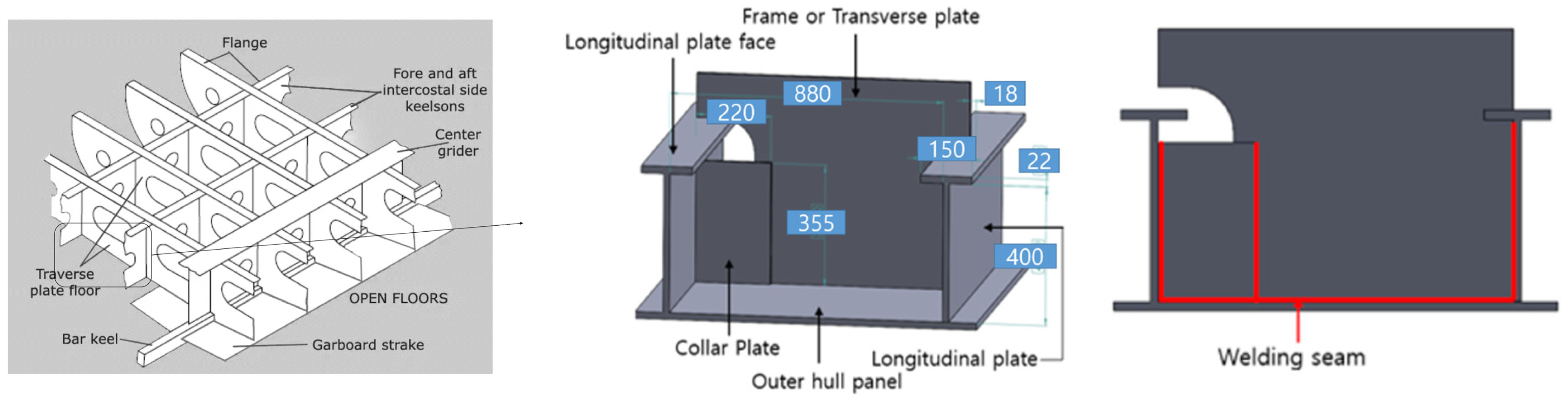
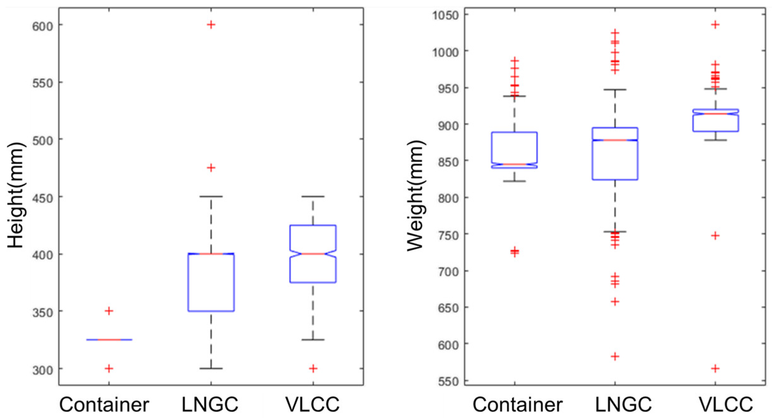
2.1. Selection of Work Object

The work object is based on the U-cell of three representative ship types built at shipyards: container ship, LNGC, and VLCC (very large crude-oil carrier) [23]. The proportion of work objects by ship type fluctuates according to global ship ordering trends, and as the number of orders for LNGCs has increased rapidly in the past two years, LNGCs also account for most of the analysis data. A total of 23,457 U-cells were analyzed, of which 90% (21,208) were LNGC, 7% (1537) were container ships, and the remaining 3% (712) were VLCC. The main analytical dimensions of the work object were Longi height and Longi width, and they were analyzed by boxplot for each type of vessel as shown in Figure 2.

Table 1. Magnitude of properties of U-cell block by ship type.

Dimension	Type	Median	Min	Max
Longi. Height (Unit: mm)	CONTAINER	325	300	350
	LNGC	400	300	600
	VLCC	400	300	450
Longi. Width (Unit: mm)	CONTAINER	845	723	987
	LNGC	880	582	1025
	VLCC	914	566	1036

shows the size of Longi by vessel type. The maximum, minimum, and median values of height and width are summarized. LNGC and VLCC had the same median height of 400 mm, and only container ships had a smaller median value of 325. In the case of width, the median value range of the three ship types was 845 to 914. LNGC, which accounted for 90% of the total volume, had a height of 400 mm and a width of 880 mm, so it can be considered a representative size of a U-cell.

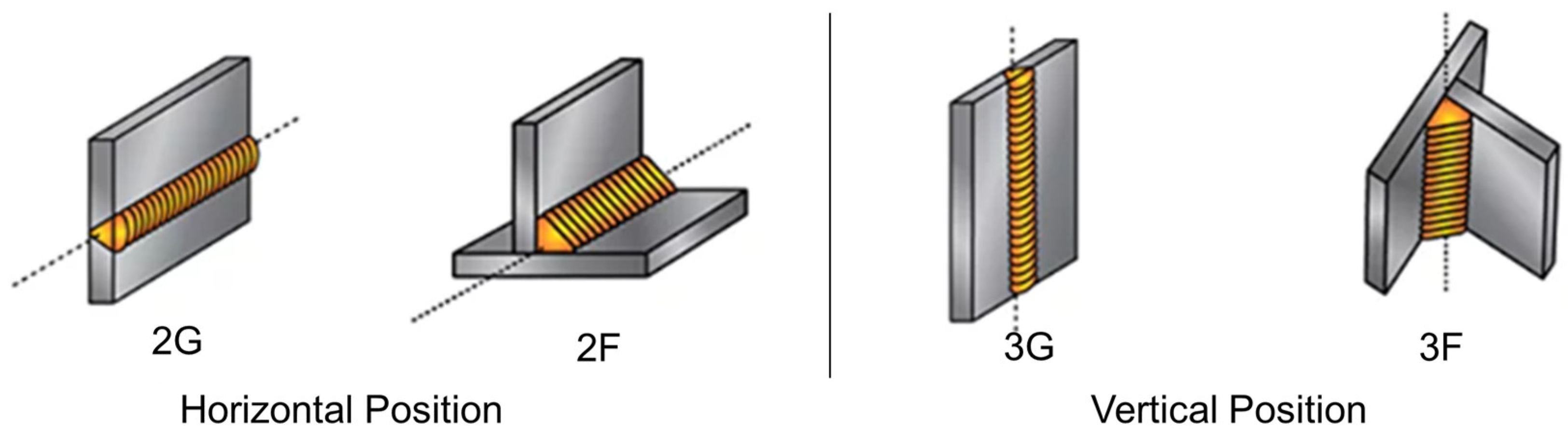
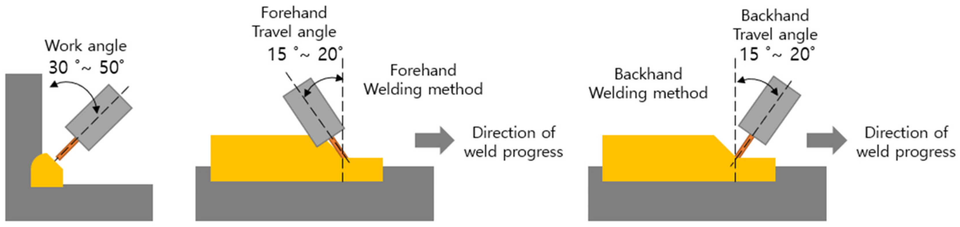
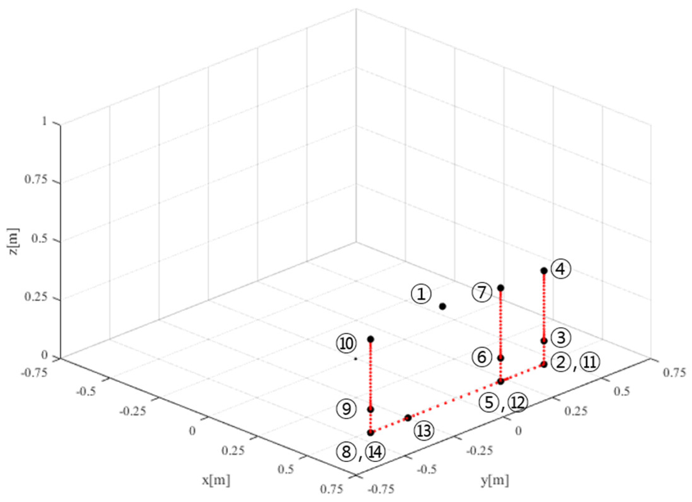
2.2. Trajectory Planning

The desired position of the robot in the task space consists of Trans, Longi, Collar plate, and Outer hull plate intersecting each other, as shown in Figure 1. The size is defined based on the analysis in Section 2.1, with the dimensions at Longi, having a height of 400 mm and a width of 880 mm. The desired orientation, as shown in Figure 3, represents the posture conditions required for welding under 2F and 3F conditions. The numbers 2F and 3F distinguish between horizontal and vertical positions during welding, while the letters F and G represent Fillet and Groove welding, respectively [24]. The workpieces in this paper are grid structures, and since all components are joined vertically, they correspond to Fillet welding.

Figure 4 delineates the forward angle technique and backward angle technique, as well as the work angle based on the welding joint criteria with respect to the welding direction. Forward and backward angle techniques are selectively used to form flat or relatively convex beads, depending on the shape and size of the gap during Groove or Fillet welding, respectively [25]. However, adjusting forward and backward angles in real-time to accommodate changing gap conditions during robot welding is practically infeasible. Therefore, from the robot’s perspective, the most neutral position, with forward/backward angles at 0°, becomes the basis for determining welding conditions. The theoretically optimal work angle to create symmetrical weld beads is 45°.

At the intersection point where the three faces of Longi, Plate, and Trans intersect, it is not feasible to position the welding torch at the ideal angle due to mechanical collisions. Therefore, the torch is given a backward angle to avoid collisions, while maintaining the work angle at 45°. The torch is rotated until a position is reached where there are no collisions, and the backward angle becomes 0°. The distance from the welding starting point to the point where the backward angle of the welding torch becomes 0° is referred to as the angle distance (AD). For vertical welding, the distance from the end of AD to the end of the welding line is called the welding distance (WD), while for horizontal welding, it is the distance from the end of the left AD segment to the start of the right AD segment.

The robot in this paper is operated after being manually moved and installed by a person. Therefore, when generating work programs, an angle distance (AD) of typically 100 mm is set to accommodate for manual installation errors, robot origin calibration errors, fabrication errors of the workpiece, and other factors.

Based on the aforementioned description, the standard welding posture conditions for the robot were as follows:

(1)

For all straight segments excluding the AD segment, the travel angle was set to 0 degrees, and the work angle was fixed at 45 degrees.

(2)

In the AD segment, to avoid collisions, the travel angle was set to 45 degrees at the starting point, and the AD was interpolated such that at the end of the AD with a distance of 100 mm, the travel angle became 0 degrees. The value of AD 100 mm was determined using commercial simulation tools (RobCAD V7.0), which take into account torch interference.

For path planning, we set a total of 14 waypoints, distinguishing between WD and AD as described above and depicted in Figure 5. The robot’s reference coordinate system was defined as [0, 0, 0] and the initial joint angles of the robot are given by ${q_{initial}}^T={[0°,20°,50°,0°,-50°,0°]}^T$ At this configuration, the position and orientation of the robot’s end-effector are represented by ${x_{initial}}^T={[0.4407,0,0.3707,0,20°,0]}^T$. Using this as the starting point, we defined the desired input for each waypoint, and to facilitate intuitive understanding, we organized this information in

Table 2. Cartesian trajectory.

No	Desired Trajectory	X (m)	Y (m)	Z (m)	Roll (°)	Pitch (°)	Yaw (°)
1	Initial	0.4407	0	0.3707	0°	20°	0
2	Left-down vertical	0.6	0.44	0	0°	45°	45°
3	Left-AD vertical	0.6	0.44	0.1	0°	0°	45°
4	Left-end vertical	0.6	0.44	0.4	0°	0°	45°
5	Collar-down vertical	0.6	0.22	0	0°	45°	45°
6	Collar-AD vertical	0.6	0.22	0.1	0°	0°	45°
7	Collar-end vertical	0.6	0.22	0.4	0°	0°	45°
8	Right-down vertical	0.6	−0.44	0	0°	45°	−45°
9	Right-AD vertical	0.6	−0.44	0.1	0°	0°	−45°
10	Right-end vertical	0.6	−0.44	0.4	0°	0°	−45°
11	Left-down horizontal	0.6	0.44	0	30°	35°	45°
12	Left-AD horizontal	0.6	0.34	0	0°	45°	0°
13	Right-AD horizontal	0.6	−0.34	0	0°	45°	0°
14	Right-down horizontal	0.6	0.44	0	−35°	30°	−54°

.

Waypoints serve as both the starting and ending points for each path, and interpolation was performed for both position and orientation between these waypoints. For position, a 3rd order polynomial interpolation was applied between each pair of waypoints. However, for orientation, which is represented by a direction vector, interpolating directly in terms of roll, pitch, and yaw could lead to singularities or imaginary numbers, resulting in incorrect interpolation. This paper used axis-angle representation for interpolating orientations instead of quaternions’ complex system, as axis-angle representation offers a more intuitive understanding of frames.

The axis-angle representation represents a rotation in three-dimensional Euclidean space with a unit vector $\overrightarrow{\mathrm{K}}={\left[k_x k_y k_z\right]}^T$ representing the direction of the rotation axis and an angle $\theta$ representing the magnitude of the rotation, as shown in Figure 6. Equation (1) is the rotation matrix consisting of the $\overrightarrow{\mathrm{K}}$, which can be used to rotate an A-frame into an a-frame by rotating it by $\theta$ about the axis $\overrightarrow{\mathrm{K}}$ [26].

$${}_a{}^{A}R_K\left(\theta \right)=\left[\begin{array}{ccc}{r}_{11}& r_{12}& r_{13}\\ r_{21}& r_{22}& r_{23}\\ r_{31}& r_{32}& r_{33}\end{array}\right]=\left[\begin{array}{ccc}{k}_x{k}_x\mathrm{v}\theta +\mathrm{c}\mathrm{o}\mathrm{s}\theta & k_x{k}_y\mathrm{v}\theta -k_z\mathrm{c}\mathrm{o}\mathrm{s}\theta & k_x{k}_z\mathrm{v}\theta +k_y\mathrm{s}\mathrm{i}\mathrm{n}\theta \\ k_x{k}_y\mathrm{v}\theta +k_z\mathrm{s}\mathrm{i}\mathrm{n}\theta & k_y{k}_y\mathrm{v}\theta +\mathrm{c}\mathrm{o}\mathrm{s}\theta & k_y{k}_z\mathrm{v}\theta -k_x\mathrm{s}\mathrm{i}\mathrm{n}\theta \\ k_x{k}_z\mathrm{v}\theta -k_y\mathrm{s}\mathrm{i}\mathrm{n}\theta & k_y{k}_z\mathrm{v}\theta +k_x\mathrm{s}\mathrm{i}\mathrm{n}\theta & k_z{k}_z\mathrm{v}\theta +\mathrm{c}\mathrm{o}\mathrm{s}\theta \end{array}\right]$$

(1)

$$\mathrm{v}\theta =1-\mathrm{c}\mathrm{o}\mathrm{s}\theta$$

(2)

$$\theta =\mathrm{a}\mathrm{c}\mathrm{o}\mathrm{s}(\frac{r_{11}+r_{22}+r_{33}-1}{2})$$

(3)

Equation (2) is the definition for $\mathrm{v}\theta$. Using the diagonal elements in Equation (1), the angle $\theta$ can be derived as shown in Equation (3).

$$\underset{K}{\to }=\frac{1}{2\mathrm{s}\mathrm{i}\mathrm{n}\theta }\left[\begin{array}{c}{r}_{32}-r_{23}\\ r_{13}-r_{31}\\ r_{21}-r_{12}\end{array}\right]$$

(4)

The computational process of trajectory planning is as follows:

(1)

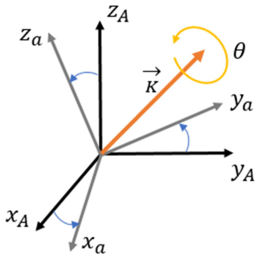
Convert the roll, pitch, and yaw angles of each row in Table 2 into a $3\times 3$ rotation matrix.

(2)

Use Equations (3) and (4) to calculate axes $\overrightarrow{\mathrm{K}}$ and $\theta$ for consecutive rows in Table 2.

(3)

Interpolate $\theta$ using a 3rd-order polynomial. Then, input the interpolated $\theta$ into Equation (1) to obtain the interpolated rotation matrices.

(4)

Utilize the n, o, and a vector of the rotation matrices, or convert the rotation matrices into roll, pitch, and yaw angles to use as the desired orientation. In this paper, roll, pitch, and yaw angles were used.

From the rotation matrices, we converted them to roll, pitch, and yaw to plan the trajectory with a total of 320 steps.

3. Design of Robot Simulator

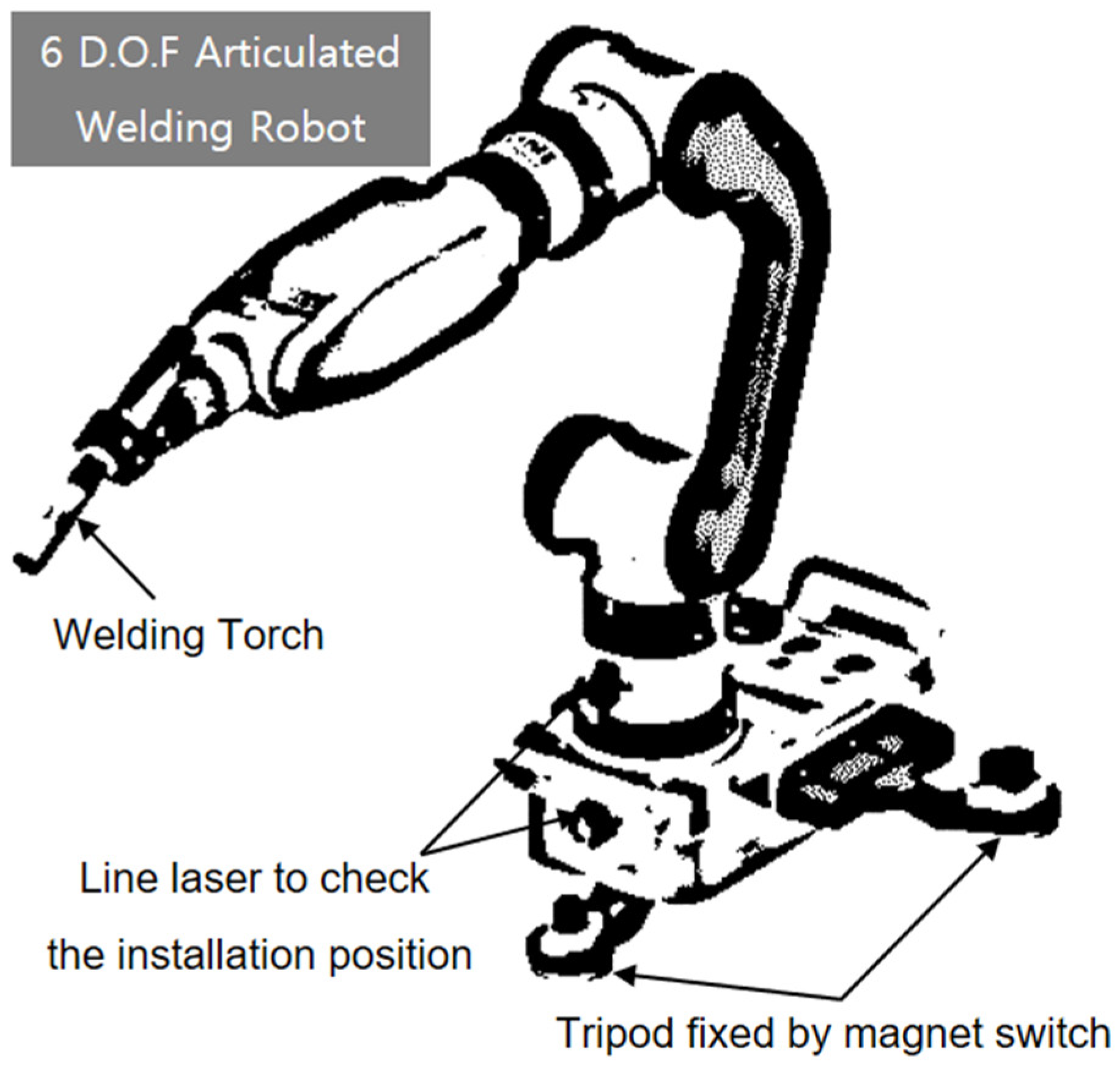
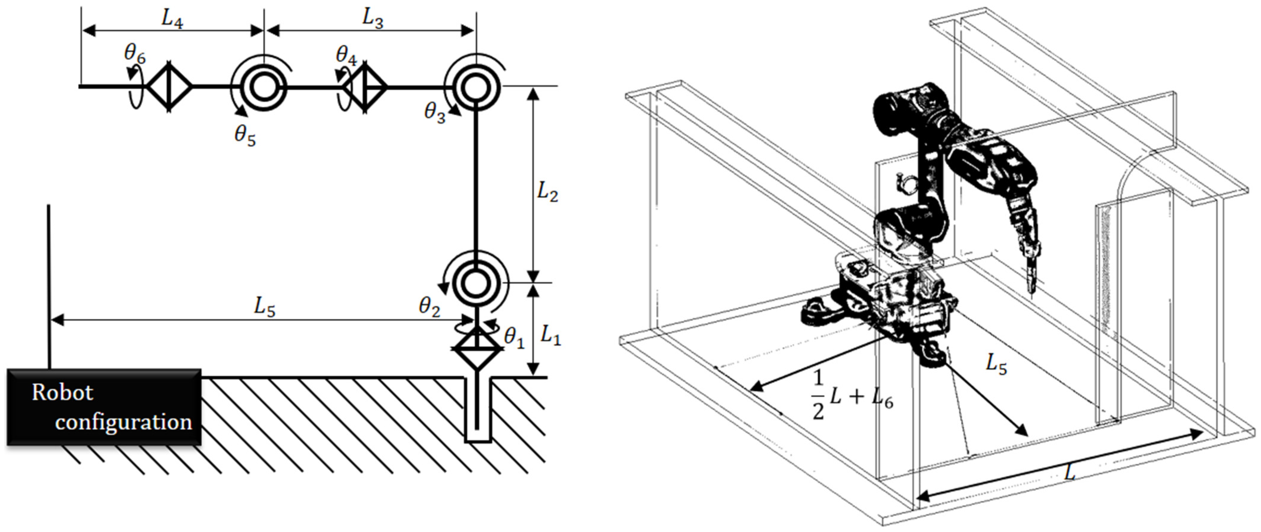
3.1. Robot Description

The designed vertical articulated robot has 6 degrees-of-freedom, weighs 15 kg, and is equipped with a manual tool changer on the end-effector to attach the welding torch as shown in Figure 7. The robot’s external design is serial, which means that the left and right motions are generated symmetrically, which is advantageous for generating motion to avoid interference in a symmetrical workspace. The robot is manually installed in the work area by a human using line lasers mounted on the front and side of the robot base and fixed on a steel plate using a magnetic switch. The installation error is compensated when the robot performs touch sensing for work object recognition [27].

The basic specifications of the robot are shown in

Table 3. Robot specification.

Type	Vertically Articulated robot
Axes	6
Payload	3 kg
Robot weight	15 kg
End-effector type	Welding torch
End-effector weight	1.6 kg (including welding cable)
Length from pivot joint to end-effector	278 mm
Axes	Joint Angle	Joint Speed
1-Axis	−150°~+150°	74.5°/s
2-Axis	−90°~+90°	74.5°/s
3-Axis	−60°~+90°	74.5°/s
4-Axis	−200°~+200°	118.8°/s
5-Axis	−90°~+90°	118.8°/s
6-Axis	−360°~360°	120°/s

. Because it is intended for welding, the joint speed is relatively slow compared to industrial robots, and it was developed with a focus on being lightweight.

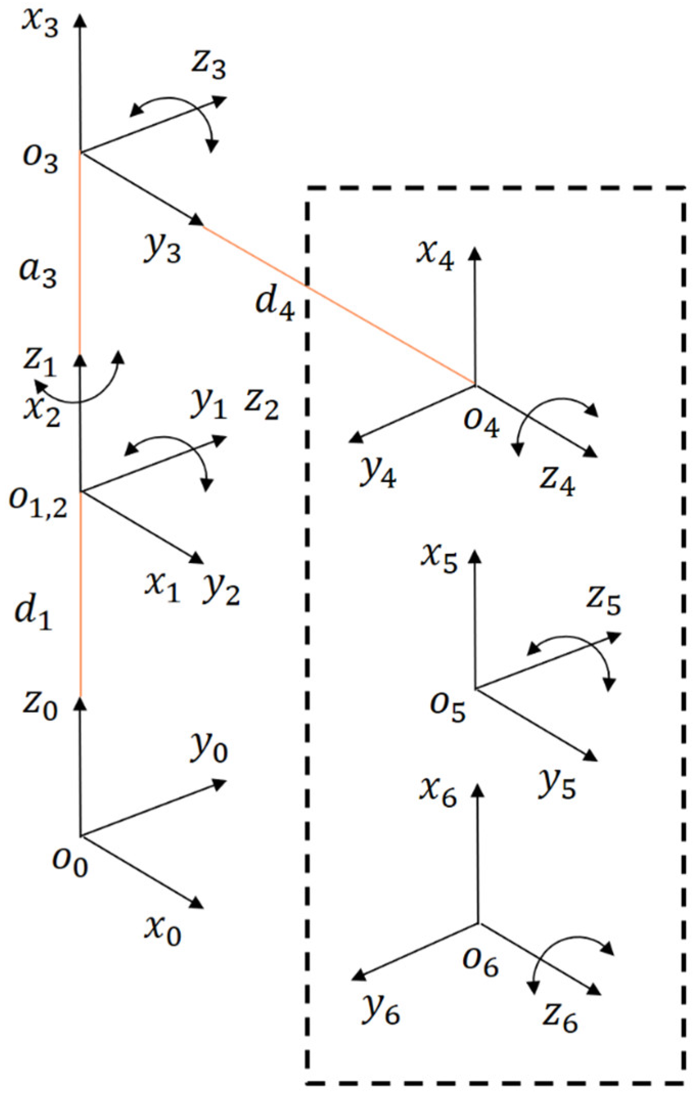
3.2. Robot Kinematics

The forward kinematics of the robot were defined by the Modified D-H (Denavit–Hartenberg) parameters [28]. The use of Modified DH in this paper was purely for convenience, as it holds the inverse kinematic solutions used as constraints in Section 4.2.3. Each joint of the robot has a rotational motion about the z-axis. Unlike the Standard D-H, the Modified D-H defines the frame by performing translations and rotations from the x-axis, followed by rotations and translations from the z-axis.

Table 4. Modified D-H parameters.

Robot	${\mathbf{a}}_{\mathit{i}-1}$	${\mathit{\alpha }}_{\mathit{i}-1}$	${\mathit{\theta }}_{\mathit{i}}$	${\mathit{d}}_{\mathit{i}}$
Joint1	0	0$°$	${\theta }_1$	d1
Joint2	0	$-90°$	${\theta }_2-90°$	0
Joint3	a3	0$°$	${\theta }_3$	0
Joint4	0	$-90°$	${\theta }_4$	d4
Joint5	0	$90°$	${\theta }_5$	0
Joint6	0	$-90°$	${\theta }_6$	0

summarizes the Modified D-H parameters. Figure 8 represents the frame configuration defined by the Modified D-H parameters.

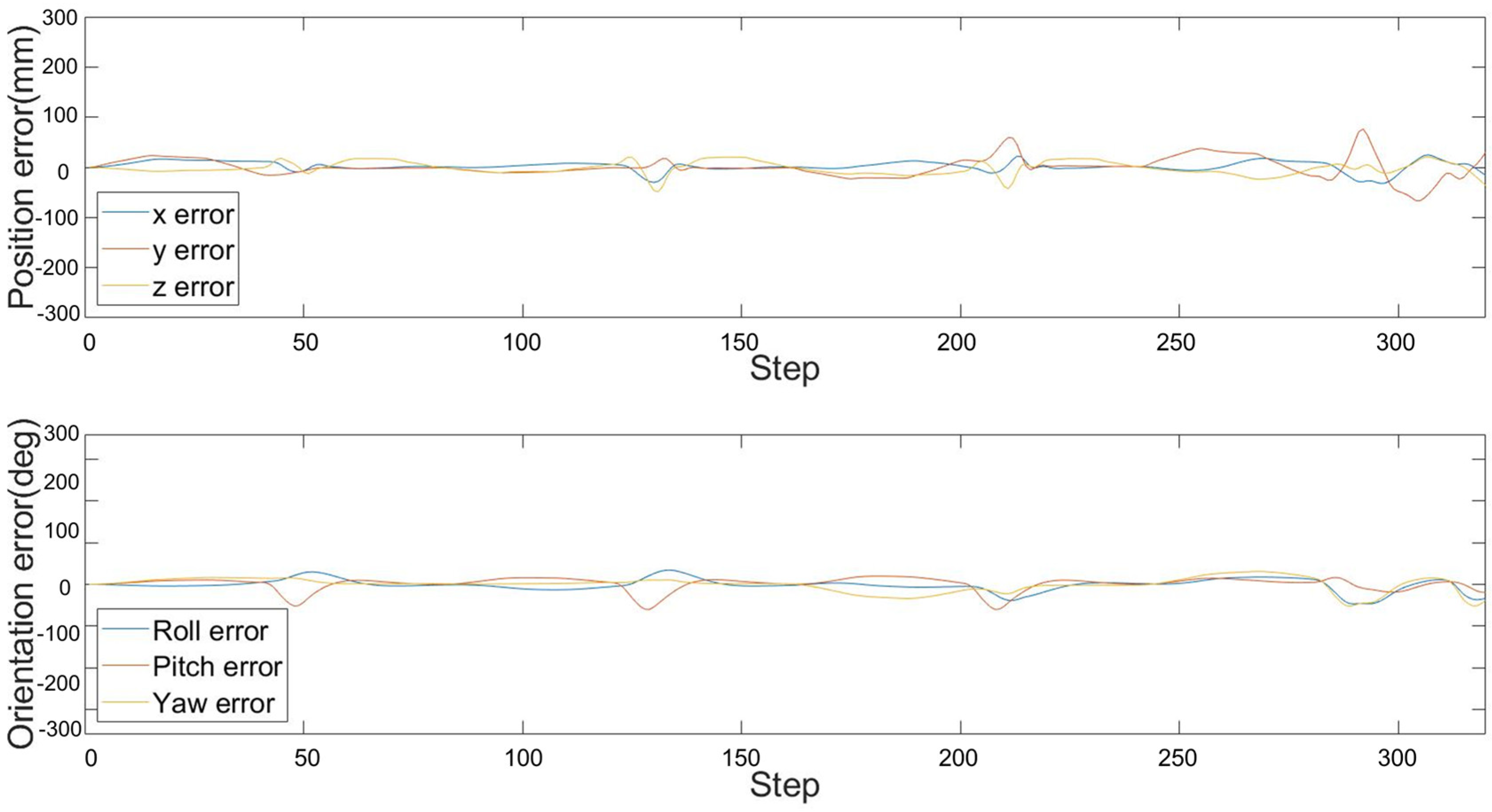
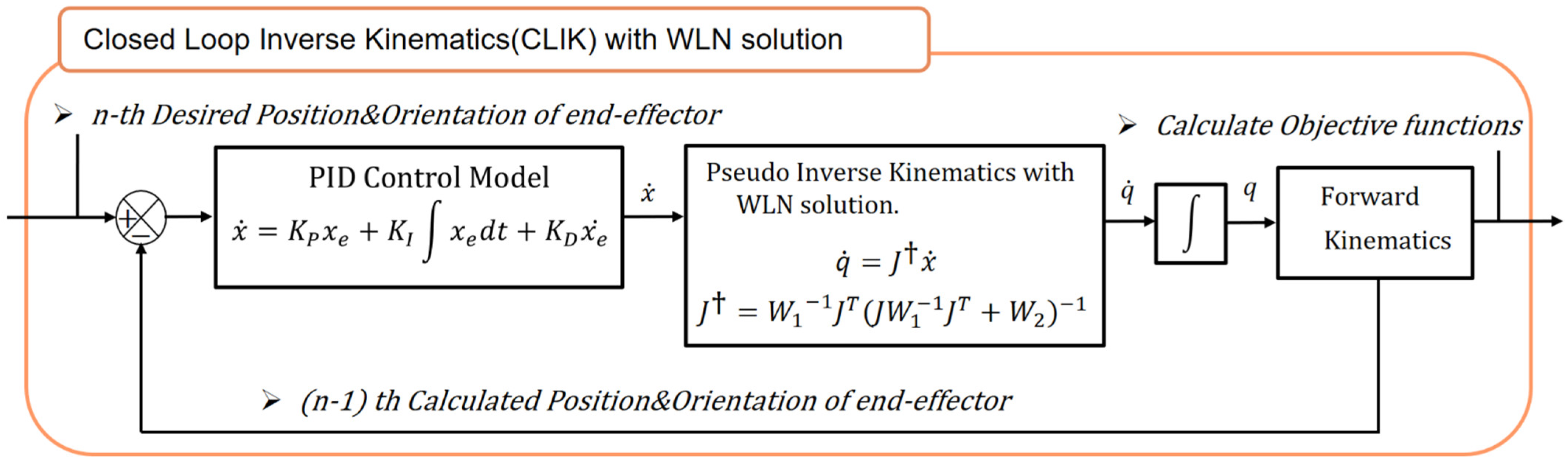
3.3. Closed-Loop Inverse Kinematics Algorithm with PID Controll and WLN Solution

The CLIK algorithm with PID controller has the advantage of simulating robot motion similar to the actual control environment [29]. However, since there is no separate restriction on the robot joint angle, we applied the WLN solution for joint angle restriction [14,16].

The robot’s Jacobian matrix is a differential kinematic matrix that defines the relationship between the task space and the joint space as shown in Equation (5). Where $\dot{x}$ is a vector of 6-degree-of-freedom linear velocity and angular velocities in the task space and $\dot{q}$ is a vector of angular velocities of the robot joints in the joint space.

$$\dot{x}=J\dot{q}$$

(5)

The Jacobian matrix consists of an $m\times n$ matrix, where $m$ is the number of degrees-of-freedom in the task space and $n$ is determined by the number of joint axes of the robot. Since the joints of the robot in this paper are all rotary joints, the composition of the rotary joint vectors in Equations (6) and (7) defines the Jacobian as shown in Equation (8). $z_i$ is the axis vector of the rotary joint, $o_n$ is the position vector from the origin to the end-effect, and $o_i$ is the position vector from the origin to the i-th joint. The pseudo-inverse matrix Jacobian is equal to Equation (9). The joint angle can be calculated by multiplying the pseudo-inverse matrix Jacobian by $\dot{x}$ and integrating it [30].

$$J_{vi}=\left\{\begin{array}{c}{z}_{i-1}\times \left(o_n-o_{i-1}\right)\\ z_{i-1}\end{array}\right.\begin{array}{c}for revolute joint i\\ for prismatic joint i\end{array}$$

(6)

$$J_{wi}=\left\{\begin{array}{c}{z}_{i-1}\\ 0\end{array}\right.\begin{array}{c}for revolute joint i\\ for prismatic joint i\end{array}$$

(7)

$$J={\left[\begin{array}{c}{z}_{i-1}\times \left(o_n-o_{i-1}\right)\\ z_{i-1}\end{array}\right]}_{m\times n}={\left[\begin{array}{ccccc}{J}_{v1}& J_{v2}& J_{v3}& \dots & J_{vn}\\ J_{w1}& J_{w2}& J_{w3}& \dots & J_{wn}\end{array}\right]}_{m\times n}={\left[\begin{array}{c}{J}_v\\ J_w\end{array}\right]}_{m\times n}$$

(8)

$${J^{†}=J^T{(JJ}^T)}^{-1}$$

(9)

The pseudo-inverse matrix Jacobian with WLN is applied with two weight matrices, the gradient matrix denoted as $W_1$ and the Damped Matrix denoted as $W_2$ in Equation (10).

$${J^{†}={W_1}^{-1}{J}^T\left(J{W_1}^{-1}{J}^T+W_2\right)}^{-1}$$

(10)

The gradient matrix $W_1$ is a diagonal matrix, as shown in Equation (11), that forces the joint angle of each joint in the joint space to be in the middle of the constrained range. $w_i$ is the weight of each joint that makes up the diagonal of the gradient matrix. In Equation (12), $\mathrm{H}/𝜕q_i$ is zero within the constrained range of each joint and increases to infinity as it approaches the joint constraint angle. Therefore, $w_i$ has a value close to infinity as the joint angle approaches the joint constraint angle, and a value of 1 as it approaches the middle of the joint constraint angle to reduce joint motion.

The damped matrix, denoted $W_2$, is also a diagonal matrix. The value of ${\lambda }^2$, which makes up the diagonal, is added to the diagonal of the Jacobian matrix, so it always creates a full rank and prevents singular solutions from occurring. The larger the value of ${\lambda }^2$, the more robust the robot is to singularities, but the less precise the robot’s control, and the smaller the value, the more precise the robot’s control, but the more vulnerable it is to singularities.

$$W_1={\left[\begin{array}{ccc}{w}_1& \cdots & 0\\ ⋮& \ddots & ⋮\\ 0& \cdots & w_6\end{array}\right]}_{6\times 6}{W}_2={\left[\begin{array}{ccc}{\lambda }^2& \cdots & 0\\ ⋮& \ddots & ⋮\\ 0& \cdots & {\lambda }^2\end{array}\right]}_{6\times 6}$$

(11)

$$w_i=\left\{\begin{array}{c}1+\left|\frac{𝜕H}{𝜕q_i}\right|if∆\left|\frac{H}{𝜕q_i}\right|\ge 0\\ 1 if∆\left|\frac{H}{𝜕q_i}\right|<0\end{array}\right.$$

(12)

$$\frac{H}{𝜕q_i}=\frac{{(q_{i,max}-q_{i,min})}^2{(2q_i-q_{i,max}-q_{i,min})}^2}{{(q_{i,max}-q_i)}^2{(q_i-q_{i,min})}^2}$$

(13)

The pseudo-inverse matrix Jacobian reflecting the WLN can be multiplied by $\dot{x}$ as a $6\times 1$ vector, which consists of the linear velocity and angular velocity vectors in the task space, to calculate the joint angular velocity in the joint space, as shown in Equation (14). The joint angle can be obtained by integration of this. The following error of the robot is calculated as the difference between $x_d$, which is a $6\times 1$ vector of desired position and desired orientation, and $x_a$, which is a $6\times 1$ vector of actual position and actual orientation, as shown in Equation (15). This following error is controlled by the PID control algorithm in Equation (16).

$$\dot{q}=J^{†}\dot{x}$$

(14)

$$x_e=x_d-x_a$$

(15)

$$\dot{q}=J^{†}(K_P{x}_e+K_D\dot{x_e}+K_I\int x_{e}dt)$$

(16)

The PID controller used in this paper aims to emulate realistic tracking errors rather than achieving optimal gain tuning. In actual industrial robots, humans often manually adjust the gain values to reduce the following error of the robot during gain tuning. Following the same approach, we iteratively adjusted the diagonal matrices $K_P$, $K_I$, and $K_D$ of the PID controller in Equation (16) in the completed simulator several times to align with the level shown in Figure 9.

Figure 10 is a diagram of the simulated control loop of the CLIK algorithm with a PID controller and WLN Solution.

4. Description of Computational Procedure

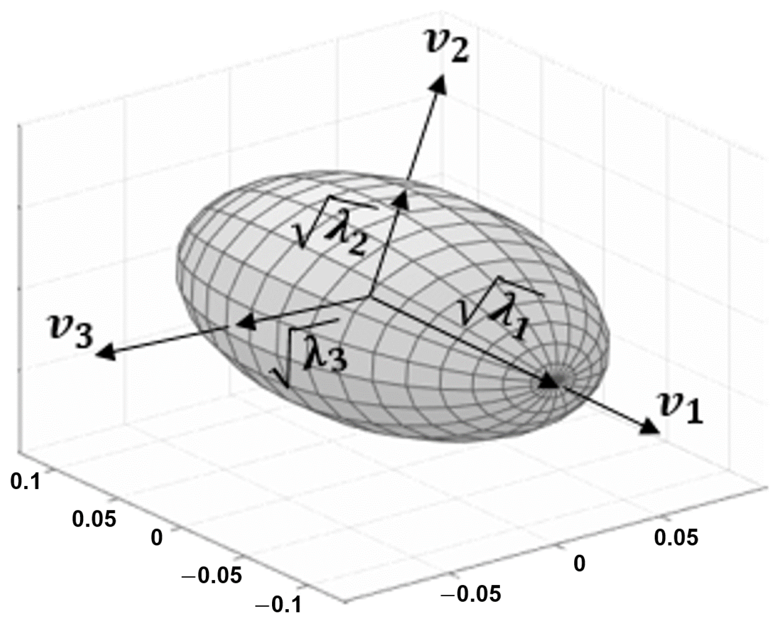
4.1. Robot Manipulability

The manipulability of a robot can be visualized and represented in the form of an ellipsoid [31] or polytope [32,33]. While the polytope method accurately describes the acceptable region in the task velocity space, it is less interpretive than the ellipse method and the computational complexity increases with the applied dimension. In this study, we evaluated manipulability using the ellipsoid method, which is better suited for interpreting.

Linear velocity manipulability evaluates how free the robot end-effector is to move its position. Angular velocity manipulability evaluates how free the robot end-effector is to change its attitude. The meaning of “free” as described here is how fast it can move and rotate. In general, to represent the manipulability ellipsoid of the robot-end, we defined an A matrix by multiplying the Jacobian and the transpose of the Jacobian, as shown in Equation (17).

$$A=J{J}^T$$

(17)

$$AS=S\lambda \Rightarrow A=S\lambda S^{-1}$$

(18)

The A matrix is a positive definite square matrix. It also has an inverse. Decomposing the A matrix as shown in Equation (18) gives a $\lambda$ matrix with the eigenvalues as diagonal elements and a S matrix with the eigenvectors corresponding to each eigenvalue as columns. In a manipulability ellipsoid as shown in Figure 11, the eigenvalue vectors represent the direction of each axis of the ellipsoid and the eigenvalues represent the length of that axis.

The manipulability of the robot can be evaluated by the following equation.

$$u_1\left(A\right)=\sqrt{\frac{{\lambda }_{max}}{{\lambda }_{min}}}\ge 1(=1 : Isotropic)$$

(19)

$$u_2\left(A\right)=\sqrt{{\lambda }_1{\lambda }_2\dots {\lambda }_n}=\sqrt{det\left(A\right)}$$

(20)

Equation (19) evaluates how close a manipulability ellipsoid is to a sphere. The closer it is to 1, the more isotropic it is. Equation (20) evaluates how large the overall volume of the manipulability ellipsoid is. For Equation (19), the value is greater than 1, and the closer to 1 the better. In the case of Equation (20), the larger the value, the better the manipulability of the robot. In this paper, we defined a bi-objective function to evaluate linear and angular velocity manipulability using the above manipulability measures.

4.2. Optimal Design Probelm

4.2.1. Definition of the Design Variables

There are six design variables: four variables related to the link length of the robot and two variables that determine the position of the robot, as shown in Figure 12. L₁ is the link length from the ground to the 2-axis frame origin, L₂ is the link length from the 2-axis frame origin to the 3-axis frame origin, and L₃ is the link length from the 3-axis frame origin to the 5-axis frame origin. L₄ is the link length from the 5-axis frame origin to the end point of the tool. L₅ is the straight-line distance from the origin of the robot’s base coordinate system to the horizontal weld line, and L₆ is the distance the robot’s base coordinate system is from the midplane between the two Longis.

4.2.2. Definition of the Objective Function

Since the objective of optimization in this study was to improve manipulability, the objective function was designed based on the evaluation of manipulability. By minimizing the magnitude of the function as shown in Equation (21), the volume of the manipulability ellipsoid can be maximized while simultaneously approaching isotropy.

$$\frac{u_1\left(A\right)}{u_2\left(A\right)}=\frac{\sqrt{\frac{{\lambda }_{max}}{{\lambda }_{min}}}}{\sqrt{\mathrm{d}\mathrm{e}\mathrm{t}\left(A\right)}}$$

(21)

The overall manipulability of the robot can be evaluated as the average of the values calculated by Equation (21) for each robot posture during the entire working step of the robot. In this paper, a bi-objective function was defined to derive the optimal design parameters that improve the performance of both linear and angular velocity manipulability. Equations (22) and (23) are defined to apply Equation (21) to linear and angular velocity manipulability, respectively, to calculate their average values.

$$minimize to\frac{1}{N}\sum _{i=1}^N\frac{\sqrt{\frac{{\lambda }_{vi max}}{{\lambda }_{vi min}}}}{\sqrt{\mathrm{d}\mathrm{e}\mathrm{t}\left(A_{vi}\right)}}$$

(22)

$$minimize to \frac{1}{N}\sum _{i=1}^N\frac{\sqrt{\frac{{\lambda }_{wi max}}{{\lambda }_{wi min}}}}{\sqrt{\mathrm{d}\mathrm{e}\mathrm{t}\left(A_{wi}\right)}}$$

(23)

Using these two objective functions, the optimal design parameters were derived through a genetic algorithm (GA).

4.2.3. Definition of the Constraints

The three constraints are the upper and lower limits of the length of each link, the range of joint angles, and the existence of an inverse kinematic solution that satisfies the desired position and orientation of the input design parameters. The reason for incorporating constraints regarding the existence of inverse kinematic solutions is to exclude combinations of design parameters in robots generated by genetic algorithms where analytic inverse kinematic solutions for desired paths and poses are not produced. The formulated optimization problem is shown in

Table 5. Optimum design problem formulation.

Find	${\mathit{L}}_1,{\mathit{L}}_2,{\mathit{L}}_3,{\mathit{L}}_4,{\mathit{L}}_5,{\mathit{L}}_6$
Minimize	$\frac{1}{N}{\displaystyle \sum _{i=1}^N}\frac{\sqrt{\frac{{\lambda }_{vi max}}{{\lambda }_{vi min}}}}{\sqrt{\det \left(A_{vi}\right)}} \frac{1}{N}{\displaystyle \sum _{i=1}^N}\frac{\sqrt{\frac{{\lambda }_{wi max}}{{\lambda }_{wi min}}}}{\sqrt{\mathrm{d}\mathrm{e}\mathrm{t}\left(A_{wi}\right)}}$
Subject to	$0.2\le L_1\le 0.4$ $0.2\le L_2\le 0.4$ $0.25\le L_3\le 0.5$ $0.15\le L_4\le 0.35$ $-0.1\le L_5\le 0$ $-0.1\le L_6\le 0.1$	${-150°\le \theta }_1\le 150°$ $-90°\le {\theta }_2\le 90°$ $-60°\le {\theta }_3\le 90°$ $-200°\le {\theta }_4\le 200°$ $-90°\le {\theta }_5\le 90°$ $-360°\le {\theta }_6\le 360°$
	$\left(1\right) \mathrm{J}\mathrm{a}\mathrm{c}\mathrm{o}\mathrm{b}\mathrm{i}\mathrm{a}\mathrm{n} \mathrm{m}\mathrm{u}\mathrm{s}\mathrm{t} \mathrm{b}\mathrm{e} \mathrm{f}\mathrm{u}\mathrm{l}\mathrm{l} \mathrm{r}\mathrm{a}\mathrm{n}\mathrm{k}$ $\left(2\right) \mathrm{t}\mathrm{h}\mathrm{e} \mathrm{i}\mathrm{n}\mathrm{v}\mathrm{e}\mathrm{r}\mathrm{s}\mathrm{e} \mathrm{k}\mathrm{i}\mathrm{n}\mathrm{e}\mathrm{m}\mathrm{a}\mathrm{i}\mathrm{c}\mathrm{s} \mathrm{s}\mathrm{o}\mathrm{l}\mathrm{u}\mathrm{t}\mathrm{i}\mathrm{o}\mathrm{n} \mathrm{m}\mathrm{u}\mathrm{s}\mathrm{t} \mathrm{b}\mathrm{e} \mathrm{a} \mathrm{r}\mathrm{e}\mathrm{a}\mathrm{l}$

.

The upper and lower limits of the length of each link and the range of joint angles were set within the range of the actual design of the robot kinematics. The inverse kinematics constraint calculates the inverse kinematics solution that satisfies the desired position and orientation with the six design parameters generated by the genetic algorithm. The inverse kinematic solution is computed analytically in the following order: 1st axis > 3rd axis > 2nd axis > 4th axis > 5th axis > 6th axis. If the joint angle solution is complex or the rank of the Jacobian is not full rank during the calculation process, the design parameter combination is excluded from the genetic algorithm. If the joint angle solution is a complex number, it means that the real solution does not exist, and if the Jacobian is not full rank, it is because the robot posture is a kinematic singularity.

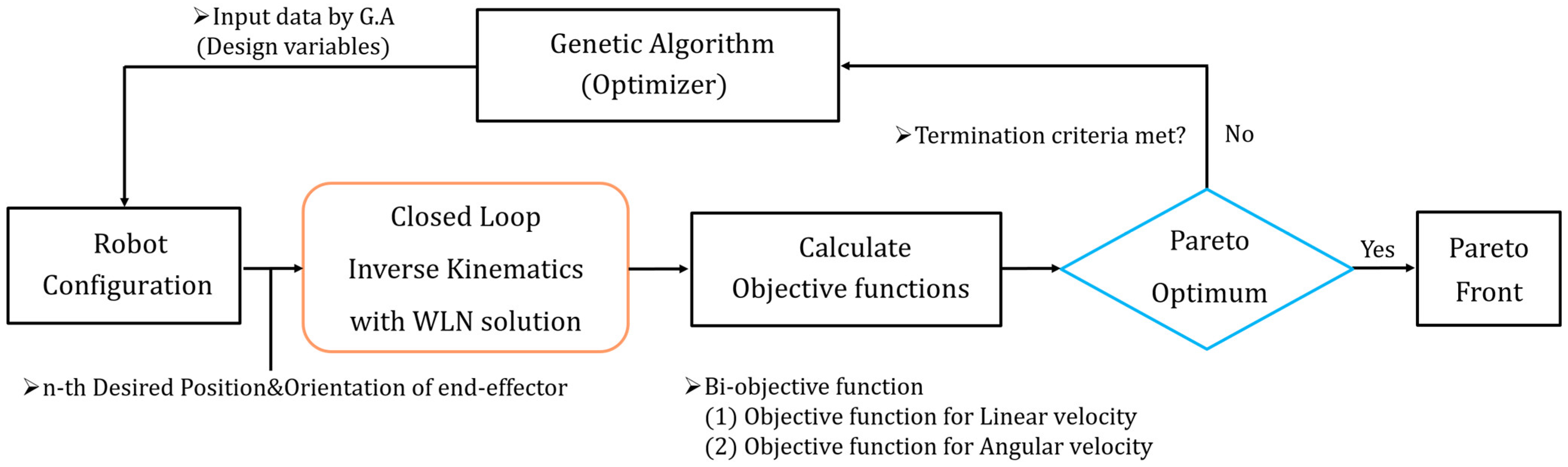
4.3. Computational Procedure for Optimizing Design Parameters

In this paper, a genetic algorithm was used to find the optimal solution [34]. Genetic algorithms are computationally time-consuming, but they have the advantage of deriving a global optimal solution that satisfies multiple objective functions. Genetic algorithms are meta-heuristic algorithms that mimic the evolutionary system in nature. Genetic algorithms essentially create multiple populations of design variables and evaluate the performance of each population every generation using an objective function that evaluates them. Each population evolves to improve its performance with each generation by performing crossover (exchanging variables between populations) or mutation (changing variables to random values) to improve performance. The population of optimal design variables derived by the genetic algorithm has improved performance compared to the initial population, and if there are multiple objective functions, the optimal design variables can be selected in a Pareto-efficient state. In this paper, the mating fraction ratio of the genetic algorithm is 0.8, the population is 200, the max generation is 70, the Pareto fraction is 0.35, the migration interval is every 20 generations, and the direction is forward. The computational procedure for deriving the optimal design solution using a genetic algorithm is shown in Figure 13.

In total, 200 populations of six random design variables, generated within the constraints of the genetic algorithm, are evaluated in a closed-loop inverse kinematics simulator with a bi-objective function for linear and angular velocity manipulability per population, and performance is improved with each generation, iteratively until the population reaches a Pareto-efficient state. A Pareto-efficient state is the state of allocation when it is impossible to make a change that benefits any one of the populations without harming the other, and can be visualized as a Pareto Front, which represents the optimal set to select the optimal solution when there are three or fewer objective functions.

5. Simulation Results

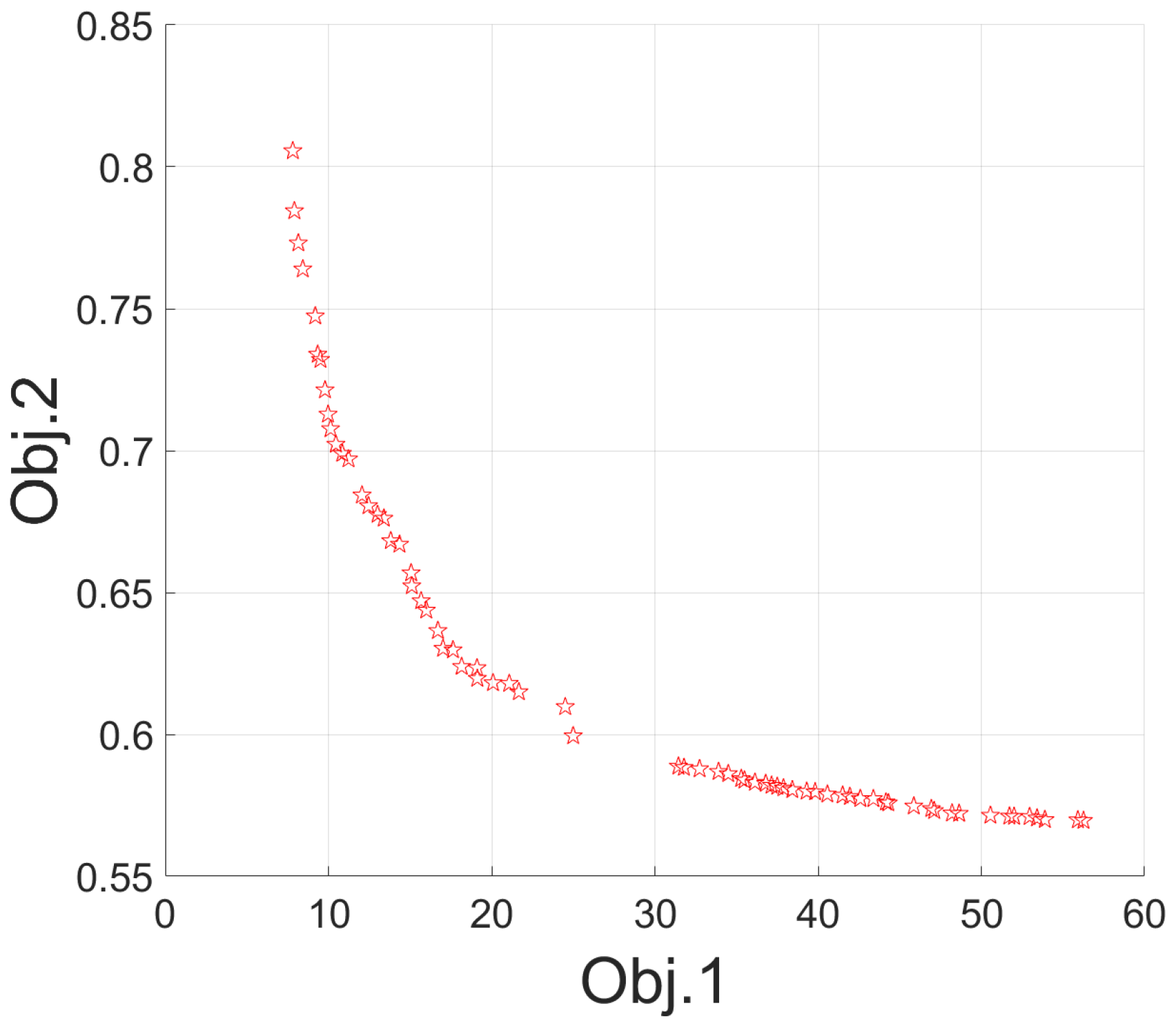
5.1. Pareto Front for Bi-Objective Function

The set of optimal solutions derived from the genetic algorithm is visualized as a Pareto front as shown in Figure 14. The horizontal axis component is the objective function for linear velocity manipulability and the vertical axis component is the objective function for angular velocity manipulability. The optimization results show that the two objective functions have a hyperbolic relationship. The solution we are looking for is the set of design variables for which each of the two objective functions is close to its minimum.

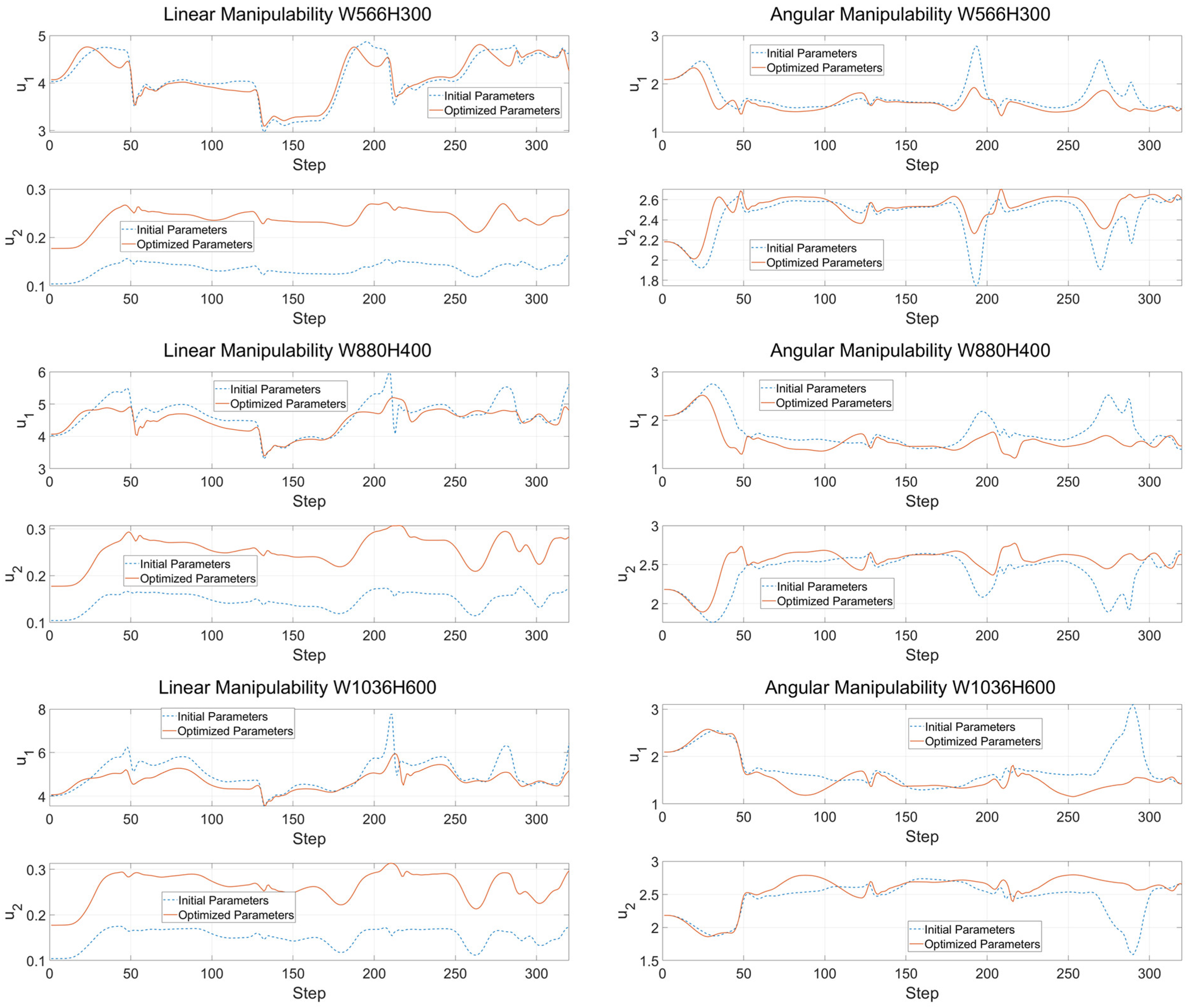
5.2. Comparison of Initial and Optimized Parameters

The optimal design variables are the population with the minimum of the two objective functions, and without any mathematical analysis, we analyzed the population of design variables within the range of variables with a horizontal axis objective function value of 20 and a vertical axis objective function value of 0.63 on the Pareto front in Figure 13. The design variables within this range were judged to have converged as the design variable sizes are almost similar as shown in

Table 6. Optimized design variables.

	${\mathit{L}}_1$	${\mathit{L}}_2$	${\mathit{L}}_3$	${\mathit{L}}_4$	${\mathit{L}}_5$	${\mathit{L}}_6$
Initial Parameters (m)	0.309	0.295	0.432	0.278	0	0
Optimized Parameters (m)	0.26	0.349	0.549	0.317	0.145	−0.015
	0.259	0.34	0.548	0.314	0.145	−0.01
	0.259	0.34	0.548	0.314	0.146	−0.009
	0.257	0.354	0.549	0.316	0.148	−0.016

.

Compared to the initial parameters, the length of the L₄ link from the pivot joint to the end-effect of the robot was shortened, but the length of the upper link L₃ and lower link L₂ was relatively longer. Among L₅ and L₆, the parameters for the placement position of the robot, L₅, the front installation distance of the robot, was 0.548 m, which is 0.062 m shorter than the existing one, and L₆, the side installation distance, was 0.009 m to the left of the middle installation distance of the member, but it is numerically close to zero. It can be interpreted that the more the robot is installed close to the center of the width of the cell, the more balanced work can be performed in the case of a robot with left–right symmetry. Figure 14 is a graph of the results of evaluating the manipulability performance for the three task objects (large, medium, and small) in Section 2.1 Table 1 for the optimal design variables [0.26, 0.349, 0.549, 0.317, 0.145, −0.015] in the first row of the optimal values in Table 6. The results were evaluated using Equations (19) and (20) to assess the isotropy and the volume of the manipulability ellipsoid.

As shown in Figure 15, the optimal design parameters show significant improvements in the range covering the entire workload per ship type. For the linear velocity manipulability evaluation, the singularities in the optimal design parameters were eliminated compared to the initial parameters, and the volume of the ellipsoid was doubled. For the angular velocity manipulability evaluation, the initial design parameters resulted in some singularities in all the workpieces, and there are some areas where the volume of the ellipsoid changes rapidly. However, in the optimal design parameters, the singularities disappeared compared to the initial design parameters, and the volume of the ellipsoid decreased rapidly.

Table 7. Comparison with initial and optimum variables.

Manipulability	Measurement	Comparison Item		W566/H300	W880/H400	W1036/H600
Linear Manipulability	$u_1\left(A\right)$	Initial	Mean	4.1298	4.6458	5.0344
			Std	0.5039	0.4975	0.6741
		Optimum	Mean	4.1162	4.4927	4.7170
			Std	0.4550	0.3732	0.4204
	$u_2\left(A\right)$	Initial	Mean	0.1359	0.1475	0.1519
			Std	0.0124	0.0180	0.0188
		Optimum	Mean	0.2392	0.2548	0.2628
			Std	0.0216	0.0300	0.0314
Angular Manipulability	$u_1\left(A\right)$	Initial	Mean	1.7415	1.7917	1.7518
			Std	0.2898	0.3366	0.3822
		Optimum	Mean	1.6204	1.5936	1.5679
			Std	0.2095	0.2599	0.3620
	$u_2\left(A\right)$	Initial	Mean	2.4347	2.3968	2.4286
			Std	0.2061	0.2384	0.2655
		Optimum	Mean	2.5119	2.5306	2.5498
			Std	0.1500	0.1834	0.2494

shows the mean and standard deviation of linear velocity manipulability and angular velocity manipulability to numerically verify the shape change and size change of the ellipsoid by workpiece size. The closer the mean of $u_1\left(A\right)$ is to 1, the more isotropic the shape of the manipulability ellipsoid is, and the smaller the standard deviation, the smaller the range of change in the shape of the manipulability ellipsoid. The larger the mean of $u_2\left(A\right)$, the larger the volume of the manipulative ellipsoid, and the smaller the standard deviation, the smaller the sudden change in volume.

To analyze the relationship between the design variables and the objective function, a correlation analysis was performed as shown in Figure 16. The length L₄ from the pivot joint to the end-effector and the distance L₅ between Trans and the robot coordinate system are positively correlated. The distance L₃ between the third axis of the robot and the pivot joint, the length L₂ between the second and third axis of the robot, and the height L₁ from the floor to the second axis are also positively correlated with the change in distance L₅. This suggests that proportionally lengthening or shortening the link length depending on the positioning distance of the robot is beneficial for manipulability. Linear velocity has an overall negative correlation with manipulability Obj.1 and the overall design variables. The shorter the length of the design variables, the more favorable the linear velocity manipulability. Angular velocity manipulability Obj.2 has an overall positive correlation with the total design variables, as opposed to linear velocity manipulability. The longer the length of the design variable, the more favorable it is for angular velocity manipulability. There is a negative correlation between the objective functions because two objective functions with conflicting correlations between the design variables must be improved simultaneously.

6. Conclusions

In this paper, we analyzed a U-cell workpiece that was created by the vertical intersection of Longi, Trans, and Plate in the double hull of a ship. The robot’s work path planning was carried out based on a work object with a Longi width of 880 mm and a height of 400 mm, which is the middle value among the analyzed work objects, and a simulation environment of a six-degree-of-freedom vertical articulated robot using CLIK with WLN and PID controller.

From Section 4 onwards, novel ideas were proposed focusing on maximizing the manipulability of the robot. The set of optimal design solutions that satisfy the constraints and the bi-objective function of the six-degree-of-freedom vertical articulated robot was visualized as a Pareto front by using a genetic algorithm for four parameters of the link length and two parameters of the robot’s installation position. The bi-objective function of the Pareto front was designed as the ratio between the shape and volume of the linear velocity manipulability and the angular velocity manipulability ellipsoid.

The optimal set of design variables visualized by the Pareto front was the set of design variables with a linear velocity manipulability objective function of 20 or less and an angular velocity manipulability objective function of 0.63 or less. The design variables in this range have similar values and are considered to have converged to near-optimal values. One of the optimal design solutions was used to compare the performance with the initial design parameters using Equations (19) and (20).

Significant improvements in linear and angular velocity manipulability were found for the optimal design parameters over the full range of work object coverage compared to the initial design parameters. For linear velocity manipulability, the elimination of singularities and the volume of the linear velocity manipulability ellipsoid were improved by a factor of two, while for angular velocity manipulability, some of the singularities were reduced and the volume of the ellipsoid changed less abruptly. A similar performance was observed for the smallest and largest workpieces.

In the future, we intend to continue research to formulate optimal design problems and derive optimal design parameters, including not only the manipulability of the robot but also the torque by axis and force/torque ellipsoid of the robot joint.

References

1. Charkraborty, S. Designing a Ship’s Bottom Structure—A General Overview. Available online: https://www.marineinsight.com/naval-architecture/design-of-ships-bottom-structure/ (accessed on 10 March 2022).
2. Kim, T.-W.; Lee, K.-Y.; Kim, J.; Oh, M.-J.; Lee, J.H. Wireless Teaching Pendant for Mobile Welding Robot in Shipyard. IFAC Proc. Vol. 2008, 41, 4304–4309. [Google Scholar] [CrossRef]
3. Ku, N.; Ha, S.; Roh, M.-I. Design of controller for mobile robot in welding process of shipbuilding engineering. J. Comput. Des. Eng. 2014, 1, 243–255. [Google Scholar] [CrossRef]
4. Kang, S.W.; Youn, H.J.; Kim, D.H.; Kim, K.U.; Lee, S.B.; Kim, S.Y.; Kim, S.H. Development of multi welding robot system for sub assembly in shipbuilding. IFAC Proc. Vol. 2008, 41, 5273–5278. [Google Scholar] [CrossRef]
5. Mun, S.; Nam, M.; Lee, J.; Doh, K.; Park, G.; Lee, H.; Kim, D.; Lee, J. Sub-assembly welding robot system at shipyards. In Proceedings of the IEEE International Conference on Advanced Intelligent Mechatronics (AIM), Busan, Republic of Korea, 7–11 July 2015; pp. 1502–1507. [Google Scholar]
6. Jacobsen, N.J. Robot welding of hatch coamings for large container ships. Ind. Robot 2007, 34, 456–461. [Google Scholar] [CrossRef]
7. Zych, A. Programming of Welding Robots in Shipbuilding. Procedia CIRP 2021, 99, 478–483. [Google Scholar] [CrossRef]
8. Jun, B.-H.; Lee, P.-M.; Lee, J. Manipulability analysis of underwater robotics arms on ROV and application to task-oriented joint configuration. In Proceedings of the MTS/IEEE Techno-Ocean ’04 (IEEE Cat No.04CH37600), Kobe, Japan, 9–12 November 2004; pp. 1548–1553. [Google Scholar]
9. Lachner, J.; Schettino, V.; Allmendinger, F.; Fiore, M.D.; Ficuciello, F.; Siciliano, B.; Stramigioli, S. The influence of coordinates in robotic manipulability analysis. Mech. Mach. Theory 2020, 146, 103722. [Google Scholar] [CrossRef]
10. Yahya, S.; Moghavvemi, M.; Mohamed, H.A. Manipulability Constraint Locus for a Six Degrees of Freedom Redundant Planar Manipulator. In Proceedings of the 2012 International Symposium on Computer, Consumer and Control, Taichung, Taiwan, 4–6 June 2012. [Google Scholar] [CrossRef]
11. Gallina, P.; Rosati, G. Manipulability of a planar wire driven haptic device. Mech. Mach. Theory 2002, 37, 215–228. [Google Scholar] [CrossRef]
12. LJin, L.; Li, S.; La, H.M.; Luo, X. Manipulability Optimization of Redundant Manipulators Using Dynamic Neural Networks. IEEE Trans. Ind. Electron. 2017, 64, 4710–4720. [Google Scholar]
13. Menasri, R.; Nakib, A.; Oulhadj, H.; Daachi, B.; Siarry, P.; Hains, G. Path planning for redundant manipulators using metaheuristic for bilevel optimization and maximum of manipulability. In Proceedings of the 2013 IEEE International Conference on Robotics and Biomimetics (ROBIO), Shenzhen, China, 12–14 December 2013; pp. 145–150. [Google Scholar]
14. Su, H.; Danioni, A.; Mira, R.M.; Ungari, M.; Zhou, X.; Li, J.; Hu, Y.; Ferrigno, G.; De Momi, E. Experimental validation of manipulability optimization control of a 7-DoF serial manipulator for robot-assisted surgery. Int. J. Med. Robot 2021, 17, 1–11. [Google Scholar] [CrossRef]
15. Jia, S.; Jia, Y.; Xu, S. Optimization algorithm of serial manipulator structure based on posture manipulability. In Proceedings of the 2016 12th World Congress on Intelligent Control and Automation (WCICA), Guilin, China, 12–15 June 2016; pp. 1080–1085. [Google Scholar]
16. Wang, J.; Li, Y.; Zhao, X. Inverse Kinematics and Control of a 7-DOF Redundant Manipulator Based on the Closed-Loop Algorithm. Int. J. Adv. Robot Syst. 2010, 7, 37. [Google Scholar] [CrossRef]
17. Colome, A.; Torras, C. Closed-Loop Inverse Kinematics for Redundant Robots: Comparative Assessment and Two Enhancements. IEEE/ASME Trans. Mechatron. 2015, 20, 944–955. [Google Scholar] [CrossRef]
18. Chan, T.F.; Dubey, R.V. A weighted least-norm solution based scheme for avoiding joint limits for redundant manipulators. In Proceedings of the 1993 Proceedings IEEE International Conference on Robotics and Automation, Atlanta, GA, USA, 2–6 May 1993; pp. 395–402. [Google Scholar]
19. Souza, D.A.; Batista, J.G.; dos Reis, L.L.N.; Júnior, A.B.S. PID controller with novel PSO applied to a joint of a robotic manipulator. J. Braz. Soc. Mech. Sci. Eng. 2021, 43, 377. [Google Scholar] [CrossRef]
20. Liu, F.; Huang, H.; Li, B.; Xi, F. A parallel learning particle swarm optimizer for inverse kinematics of robotic manipulator. Int. J. Intell. Syst. 2021, 36, 6101–6132. [Google Scholar] [CrossRef]
21. Goldberg, D.E. Genetic Algorithms in Search, Optimization & Machine Learning; Addison-Wesley: Boston, MA, USA, 1989. [Google Scholar]
22. Ngatchou, P.; Zarei, A.; El-Sharkawi, A. Pareto Multi Objective Optimization. In Proceedings of the 13th International Conference on, Intelligent Systems Application to Power Systems, Arlington, VA, USA, 6–10 November 2005; pp. 84–91. [Google Scholar]
23. Raunek. A Guide to Types of Ships. Available online: https://www.marineinsight.com/guidelines/a-guide-to-types-of-ships/ (accessed on 10 March 2022).
24. Miller. What Are the 4 Basic Welding Positions and When Should You Use Them? Available online: https://www.millerwelds.com/resources/article-library/what-are-the-4-basic-welding-positions-and-when-should-you-use-them/ (accessed on 5 May 2022).
25. MachineMFG. What Is the Effect of Welding Direction and Angle on Weld Formation. Available online: https://www.machinemfg.com/effect-of-welding-direction-and-angle-on-weld-formation/ (accessed on 5 May 2022).
26. 3D Rotations. Available online: http://motion.pratt.duke.edu/RoboticsSystems/3DRotations.html (accessed on 2 June 2022).
27. Gao, F.; Chen, Q.; Guo, L. Study on arc welding robot weld seam touch sensing location method for structural parts of hull. In Proceedings of the 2015 International Conference on Control, Automation and Information Sciences (ICCAIS), Changshu, China, 29–31 October 2015; pp. 42–46. [Google Scholar]
28. Granja, M.; Chang, N.; Granja, V.; Duque, M.; Llulluna, F. Comparison between Standard and Modified Denavit-Hartenberg Method in Robotics Modeling. In Proceedings of the 2nd World Congress on Mechanical, Chemical, and Material Engineering (MCM’16), Budapest, Hungary, 22–23 August 2016. Paper No. ICME 118. [Google Scholar]
29. Jin, S.; Lee, S.K.; Lee, J.; Han, S. Kinematic Model and Real-Time Path Generator for a Wire-Driven Surgical Robot Arm with Articulated Joint Structure. Appl. Sci. 2019, 9, 4114. [Google Scholar] [CrossRef]
30. Spong, M.W.; Hutchinson, S.; Vidyasagar, M. Robot Modeling and Control, 1st ed.; John Wiley & Sons, Inc.: Hoboken, NJ, USA, 2020; pp. 114–144. [Google Scholar]
31. Yoshikawa, T. Manipulability of Robotic Mechanisms. Int. J. Robot. Res. 1985, 4, 3–9. [Google Scholar] [CrossRef]
32. Long, P.; Padir, T. Evaluating Robot Manipulability in Constrained Environments by Velocity Polytope Reduction. In Proceedings of the 2018 IEEE-RAS 18th International Conference on Humanoid Robots (Humanoids), Beijing, China, 6–9 November 2018; pp. 1–9. [Google Scholar]
33. Chand, D.R.; Kapur, S.S. An Algorithm for Convex Polytopes. J. ACM 1970, 17, 78–86. [Google Scholar] [CrossRef]
34. Midhra, S.; Sahoo, S.; Das, M. Genetic Algorithm: An Efficient Tool for Global Optimization. Adv. Comput. Sci. Technol. 2017, 10, 2201–2211. [Google Scholar]
Figure 1. U-cell weld lines created inside the double hull of a ship.
Applsci 14 03384 g001
Figure 2. Boxplot of height and width of U-cell block by ship type.
Applsci 14 03384 g002
Figure 3. Welding position code for horizontal and vertical fillet.
Applsci 14 03384 g003
Figure 4. General technical knowledge of welding angles—work angle (left) and forehand travel angle (center), backhand travel angle (right).
Applsci 14 03384 g004
Figure 5. Interpolated position points. (The numbers within circles represent the sequence of the Desired Trajectory in Table 2).
Applsci 14 03384 g005
Figure 6. Axis-angle representation based on Euler’s rotation theorem, which rotates from A-frame to a-frame by rotating about the axis vector K by an angle θ .
Applsci 14 03384 g006
Figure 7. Hand-carried 6-degree-of-freedom vertical articulated welding robot (detailed image not available due to confidentiality reasons).
Applsci 14 03384 g007
Figure 8. Coordinate systems: D-H modified.
Applsci 14 03384 g008
Figure 9. Following error to simulate reality.
Applsci 14 03384 g009
Figure 10. Diagram of the simulated control loop of the CLIK algorithm with PID controller and WLN Solution.
Applsci 14 03384 g010
Figure 11. Manipulability ellipsoid visualized by the eigenvalues and eigenvectors on task space.
Applsci 14 03384 g011
Figure 12. Design variables: 4 robot link length variables and 2 robot placement position variables.
Applsci 14 03384 g012
Figure 13. Computational procedure to find the optimal design variables.
Applsci 14 03384 g013
Figure 14. Pareto front with the set of optimal solutions derived through genetic algorithms.
Applsci 14 03384 g014
Figure 15. Linear and angular velocity manipulability evaluation results by work object size.
Applsci 14 03384 g015
Figure 16. Correlation analysis between each design variable and objective function.
Applsci 14 03384 g016