Optimizing Mobile Laser Scanning Accuracy for Urban Applications: A Comparison by Strategy of Different Measured Ground Points

Abstract

Mobile mapping systems are part of modern data collection in geodesy. It is one of many surveying methods where field collection is performed in a short time. Among their advantages are cost savings and better visualisation than classic surveying methods. This article is focused on accuracy determinations in urban built-up areas of mobile laser scanning using the Riegl VMX-2HA system. These areas, where there is a combination of dense housing and trees, are an integral part of cities. Their diversity and complexity make surveying by other surveying methods time-consuming and complicated. In particular, the GNSS RTK method encounters problematic locations where sky obscuration by surrounding elements reduces measurement accuracy. Data collection was performed on a test base in the city of Pilsen, Czech Republic. The base includes 27 control points and more than 100 checkpoints. Two sets of coordinates were created for the points; the first set is calculated using tied net adjustment and the second one is determined by RTK GNSS measurements. Point cloud calculations were processed in RiPROCESS software from Riegl, using different configurations and qualities of the control points. Each point cloud was analysed including the determination of point cloud deviations. This article is also dedicated to the identification of problematic spots, where measurement can be degraded. The results presented in this paper show the influence of the quality and different spacing of the control points on the point cloud, its accuracy compared to the precise points, and the global and local deformation of the point cloud. This work can be used as a basis for replacing classical surveying methods with a more efficient mobile laser scanning method.

1. Introduction

At a time of great technological growth, accelerating computers, and automation, the replacement of human labour with newer instruments and processes is becoming more and more common in surveying. The level of current technologies allows the collection of big data in a very short time and moving most of the surveying work to the office. It is possible mainly due to digital photogrammetry [1,2] and laser scanning [3,4]. Combining these methods is commonly used in modern systems called mobile mapping systems [5,6,7,8]. Whether they are handheld systems [9] or systems placed on various carriers (cars, aeroplanes) the main part of these systems is INS (inertial navigation system), which is used to determine the relative position of the device, and very often they are equipped with GNSS (Global Navigation Satellite System) equipment for absolute positioning. The main output of mobile mapping is a point cloud.

The first mobile scanners appeared in the 1980s. These systems were developed for rapid GIS (Geographic Information System) data collection; they recorded spatial data using analogue cameras and determined the position of the vehicle by georeferencing the ground points and using gyroscopes, accelerometers, and odometers [10]. Development progressed, and so, as early as 1988, the Canadian MHIS (mobile highway inventory system) came along, using differential GPS (Global Positioning System) measurements combined with an inertial system to determine the position of the vehicle. Thus, the accuracy of vehicle positioning was in the tens of centimetres [11]. The next device, VISAT (Video cameras, an Inertial system, and Satellite GPS receivers), was designed to achieve a positioning accuracy of 0.3 m and a relative accuracy of 0.1 m at a speed of 60 km/h. This system already used several colour CCD (charge-coupled device) cameras to record image data [10]. The major milestone that brought mobile mapping to humanity’s awareness was the creation of Street View primarily by Google in Google Maps. This type of spatial data viewing still enjoys great popularity. Since the new millennium, LiDAR (Light Detection and Ranging) technology has been added not only to terrestrial mobile mapping systems, but also to airborne scanners, and the systems are becoming more and more advanced [12].

This article focuses on the determination of the characteristics of the mobile laser scanner RIEGL VMX-2HA’s [13] measurements in the urban build-up area. The environment in these districts is very variable. However, these are often parts of the city where there is dense residential development, tall buildings, and street trees. Other survey methods such as GNSS RTK or total station surveying are difficult and time-consuming. The first problem is the actuality of the data. Typically, these methods require a lot of field measurement time, and a large area such as a city would require months of measurements. Another problem is the complexity of the environment. For example, GNSS RTK measurements are problematic because the environment obscures the view of the sky, interferes with the GNSS signal, or cannot be used to measure points on private land without the owner’s consent.

The motivation for this project is the possibility of replacing the surveying of objects by the traditional geodesy methods with the more effective method of mobile mapping. The best-known mobile mapping systems include devices from GEOSLAM, Leica, Trimble, Faro, or GreenValley [9,14,15,16,17]. These are generally handheld devices, but most of the newer models can be mounted on various carriers. Mobile mapping devices cost from tens of thousands to hundreds of thousands of euros. Currently, short training of a non-professionally educated person is usually required to operate these systems, or it can be placed on autonomic carriers [18]. This leads to cost savings and the extension of this method to new branches [19,20]. Furthermore, the amount and type of data collected allow for more complex data analysis and visualisation, for example, in a virtual BIM environment [21,22,23].

As mentioned above, mobile mapping systems are used in many areas, not only in surveying. Handheld mobile scanners are suitable for measuring the dimensions of buildings, especially in old or complex buildings where manual measurement takes a significant amount of time. Mobile scanners are very useful in tight and poorly lit spaces, sewers, and mines, where data on the entire object can be obtained quickly. The data obtained in this way may not only be used for drawing 2D plans but they are suitable for 3D object modelling. Mobile mapping systems, where a carrier is a car, are used for mapping horizontal and vertical road signs, as sources for making Digital Technical Maps whose accuracy corresponds in Czechia to class 3 (the mean coordinate error is 14 cm), or they are used for linear structures surveying. A big issue in mobile mapping is accuracy. In particular, the dependence of accuracy on the frequency and distribution of control points [24,25].

As this is a relativity new technology that is constantly rapidly developing, it is necessary to test this method and the behaviour of the devices in real conditions. With each instrument and new software, the accuracy and reliability parameters of the output change. A large amount of the literature has been written on mobile scanning, but only a small part of it has dealt with mobile mapping systems of the type Riegl VMX-2HA. The work [26] compares mobile scanners in a point field that is 1.7 km long with a ground control point density of 1 point per 200 m. The determined accuracy is calculated from the differences between the measured MMS point cloud and the point cloud measured by the terrestrial static scanner and is around 2 cm. The papers [24,27] deal mainly with comparisons between an MMS cloud and another cloud obtained by scanning with another device, dealing with point densities and relative accuracies. The calculated standard deviations are in the range of millimetres.

The article [28] already deals with the accuracy against points measured by GNSS RTK (the spatial accuracy of a point is 7.4 cm), and a test area included up to 200 control points. The resulting mean standard deviations in this project ranged from 1.2 cm to 5.9 cm, with a maximum of 26 cm. It is important to mention that both checkpoints and MMS measurements are dependent on the GNSS method and the accuracy is of the same precision. Thus, the GNSS error is also reflected in the MMS accuracy result. Absolute accuracy is the focus of the paper [25]. In this paper, only a small area is surveyed, but the point field is dense and well-signalled, and the coordinates are accurately measured by an independent method. The standard deviation determined in this article is 1.7 cm. However, such conditions and precise points are impossible to achieve in practical use.

This project aims to simulate commercial measurements (point field accuracy and signalling) as much as possible, and it is necessary to determine the accuracy of the final point cloud depending on the measurement conditions, location, and computational parameters. Multiple parameters enter the final quality and accuracy. The most influential are the accuracy of GNSS/INS and the accuracy and spacing of the control points. The goal of the project should be to determine the overall accuracy of the mobile mapping system, the problem spots in the measured locations, and the appropriate spacing of the control points.

This article consists of several important parts. The first describes a detailed description of the testing, the devices used and their properties, the test field, the accuracy of the determination of the ground control points and checkpoints, and the expected accuracy of the MMS. Next, the chapter deals with how MMS data are processed and the approaches to their evaluation. The other section is devoted to the results, showing the calculated deviations and comparison of the measured clouds. This is then followed by a Section 4, where the determined point clouds’ properties and the ground control point strategy are verbally evaluated.

2. Materials and Methods

This chapter is dedicated to information about the testing device, test field, and the work that led to the creation of the resulting clouds. The first part focuses on the characteristics and accuracies specified by the manufacturer of the RIEGL VMX-2HA mobile mapping device with which the entire measurement was carried out. Especially from this information, an estimate of the resulting expected accuracy was made. In the next part, we describe the test point field and point stabilisation, a method of determining the coordinates and resulting accuracies of the point field. The last chapter is devoted to the work with the measured data. Specifically, the conditions and parameters of the measurements, the processing of MLS data, and a description of the evaluation method.

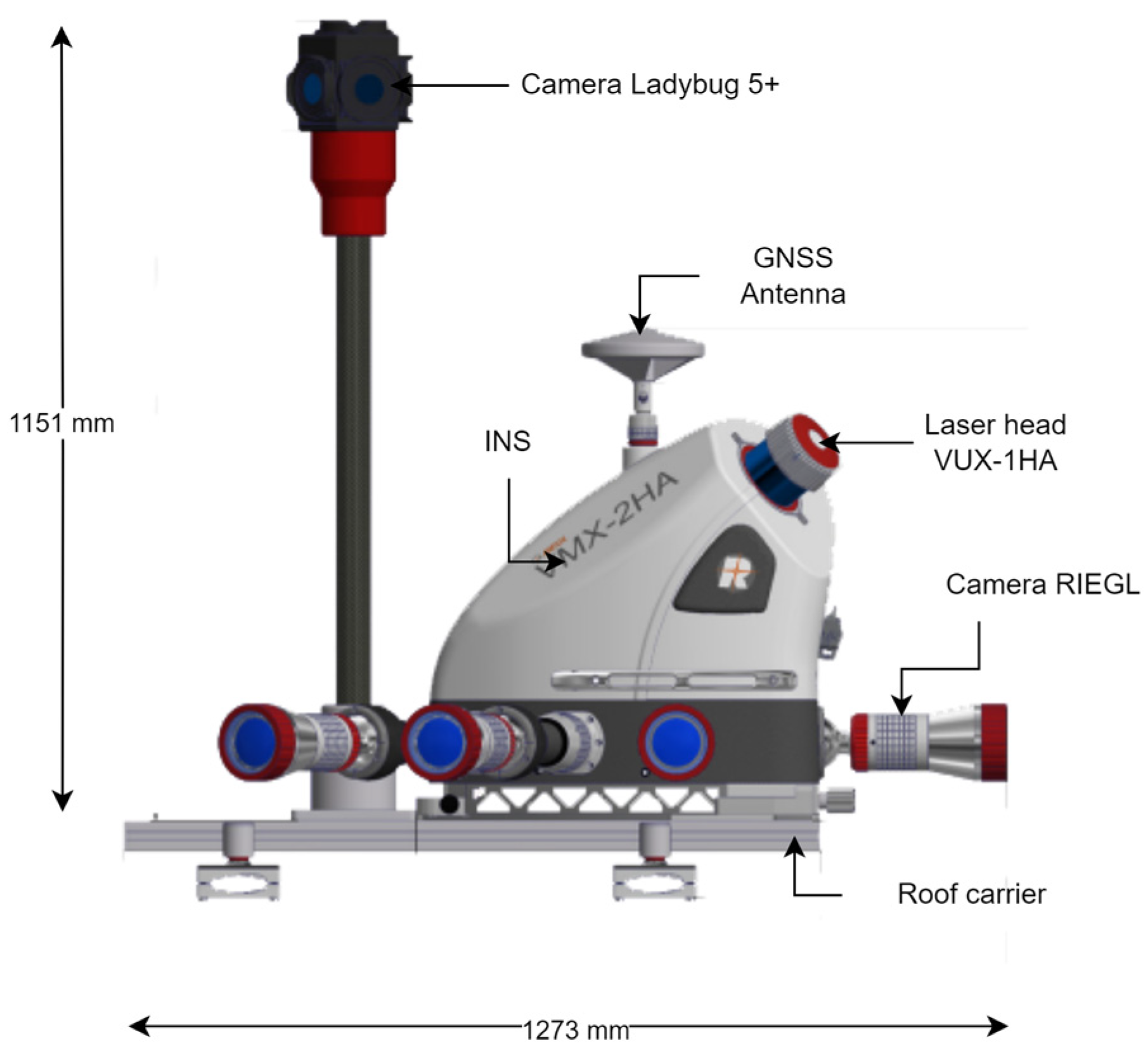
2.1. Mobile Mapping System RIEGL VMX-2HA

The VMX-2HA [13] (Figure 1) mapping system from Riegl is based on two VUX-1HA [29] laser heads with different rotation axes, capable of measuring up to 475 m, and an INS/GNSS unit [30] supplemented by an odometer (DMI). The system can be equipped with up to nine position cameras, which can be set in the required directions (depending on the object of interest), and a Ladybug 5 + panoramic camera [31], suitable for point cloud colouring. The entire system is on a carrier attached to the car.

In the product datasheet [13], the manufacturer lists several important parameters of the device.

Table 1. Point density at a laser pulse rate of 1000 kHz.

Carrier Speed	Point Density 1 Distance 3 m	Point Density 1 Distance 10 m	Point Density 1 Distance 50 m
50 km/h	13,750	4100	820
80 km/h	8590	2570	510

¹ points/m².

shows the cloud densities for a specified distance at various speeds, which may be suitable for many applications but not for this work. As mentioned in the “MLS Data Acquisition” Section 2.5, the carrier speed was lower in this test. In the first instance, the speed was 20 km/h, which was chosen for its sufficient accuracy for testing and smoothness of data collection; the same speed is used in [25], where the final accuracy is high. A simple calculation shows that the density of points at 10 m should be 10,250 points/m². In the second case, the speed was about 35 km/h, which is the average speed that could be reached in such a densely built-up environment. The calculated point density value is 5860 points/m².

Table 2. Information from the VMX-2HA datasheet.

Accuracy/repeatability of laser head	5 mm/3 mm
GNSS accuracy—horizontal/vertical	20 mm/30 mm
Pitch and roll accuracy	0.0025°
Compass accuracy	0.015°

lists the accuracy of each sensor from the manufacturer’s product datasheet. Accuracies are given for ideal conditions: an uncovered view of the sky, a maximum measured distance with a laser head to a distance up to 30 m, and the system must use a DMI (odometer).

2.2. Test Field Specification

The object of interest is to test the system in an urban area where the GNSS signal is jammed by surrounding trees and buildings. For this purpose, an extensive test field has been created to satisfy this condition [25,28]. The network is made up of control points, which are used to precisely align the point cloud, and of checkpoints.

Other important factors in selecting the location of the test field were a low-traffic site and a close location to the GEOREAL surveying company, which owns the device being tested.

Two sets of coordinates were created for all points in the test field. The first set is the coordinates determined by the dual GNSS RTK measurements and the arithmetic average (GNSS points). This method of determining points is used in real data collection. The second set of coordinates was calculated by adjustment of the tied grid from the total station measurements (TS points). The more accurate (TS) coordinates were created to be an order of magnitude more accurate than the expected accuracy of the method; see the chapter “Expected Accuracy”.

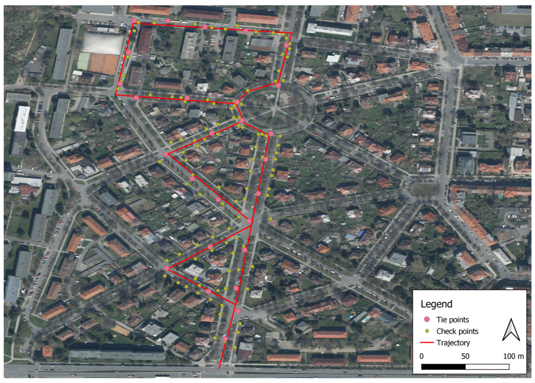
2.2.1. Test Field Parameters (Figure 2)

• Location: Plzeň—Jižní Předměstí, Na Hvězdě;
• Length of section: 1.5 km;
• Number of control points: 27;
• Number of checkpoints: approximately 90.

2.2.2. Control Points

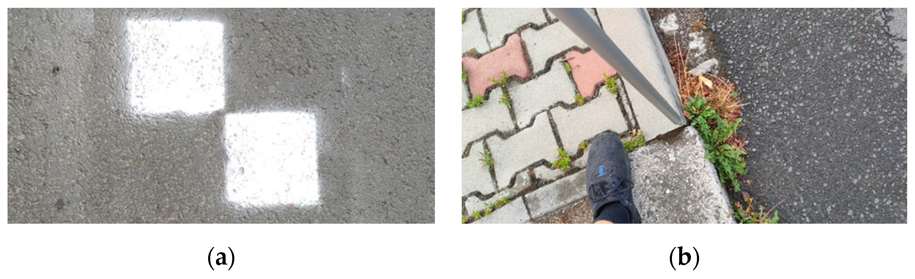
A point field with a point spacing of approximately 50 m was created at the locality. The control points were stabilised with a metal nail and signalled with a 15 × 15 cm chequerboard target (Figure 3), or they were marked as corners of horizontal road markers.

2.2.3. Checkpoints

Permanently stabilised spatial points were selected as checkpoints. These are mainly the corners of the kerbs (Figure 3), sewer shafts, and traffic signs. These types of points are often the object of interest in geodetic mapping. A checkpoint coordinate set measured by a total station was used to evaluate the accuracy of the clouds. The coordinate set determined by the GNSS method is used to compare the accuracy of the GNSS RTK method with the mobile mapping method.

2.2.4. Coordinates Determined by GNSS

The points were measured independently twice with a Leica GS18. The average standard deviations of the GNSS point determinations were calculated from the dual measurements. Standard deviations from the dual measurements of the GNSS coordinates of the points are presented in

Table 3. Standard deviations calculated from dual-point measurement.

Coordinate	Control Points	Check Points
X	13 mm	22 mm
Y	11 mm	21 mm
Z	12 mm	30 mm
XY	17 mm	31 mm
XYZ	21 mm	43 mm

.

2.2.5. Coordinates Determined by Adjustment

The control points were measured using the polygon method with a Leica TS1200 (Leica Geosystems, Heerbrugg, Switzerland) and the measurements were adjusted in the EasyNET software (Version 3.5) using the tied network method. Points 1, 5, and 25 were chosen as fixed points because they are in a position with a good view of the sky. This is crucial because it ensures clear reception of satellite signals used to determine point positions and increases the number of satellites used to calculate the position. As a result, their deviations from the GNSS measurements were minimal and the resulting coordinates are more reliable. At these points, the number of satellites was between 30 and 34. The output values of the adjustment are shown in

Table 4. Accuracy evaluation of control points adjustment.

Coordinate	Average Standard Deviation
X	1.4 mm
Y	1.7 mm
Z	0.2 mm
XY	2.2 mm
XYZ	2.2 mm

. Since the network has been measured repeatedly and many redundant measurements are available, the number of excluded measurements can be considered insignificant.

The checkpoints were surveyed twice using the polar method from the points of the adjusted grid. The maximum difference between the two coordinates is 5 mm.

2.3. Point Identification Precision from the Point Cloud

The chapter describes how accurately points can be identified from point clouds. The points were again divided into control points and checkpoints. The control points are signalised, and there should be no significant problem in identifying them. However, identification is, in many cases, more difficult for checkpoints. The corners of the features are sometimes determined from the potential intersection of the object’s edges, or they are rounded due to time. For both types, five points were selected, and these were identified ten times with time intervals in the RiPROCESS software (Version 1.9.3., Riegl, Horn, Austria).

Table 5. Accuracy of point identification precision.

Coordinate	Control Points	Check Points
X	2 mm	6 mm
Y	2 mm	4 mm
Z	3 mm	6 mm
XY	3 mm	8 mm
XYZ	4 mm	9 mm

shows the average standard deviations of the identification of the points.

2.4. Expected Accuracy

This chapter is dedicated to accuracy, which, according to the available material, can be expected. The manufacturer provides (Table 2), for ideal conditions, a laser head accuracy of 5 mm and GNSS of 20 mm in the horizontal direction and 30 mm in the vertical direction. However, these are not the only variables that affect the resulting accuracy. Others such as the INS and DMI system, the spacing of the insertion points, the type of alignment, the speed, and, above all, the fact that the measurement is not carried out under ideal conditions enter the calculation.

Compared to the paper [25], which reports a 3D standard deviation of 1.7 cm, a worse accuracy can be expected. The authors used a significantly denser point field of control points with high accuracy, and the checkpoints were very well signalised and marked with a chequerboard target. It follows from this article that the accuracy of MLS under very good conditions using precisely defined points may be better than that claimed by the manufacturer.

The option of a small spacing of the control points is not economical in real mapping in built-up areas, and the checkpoints in this project are chosen as objects of interest for mapping. Spatial points may be less easy to identify.

Also, the testing conditions in this article are not ideal according to the manufacturer’s datasheet, the view of the sky is often obscured, and we can expect worse GNSS accuracy. As the work evaluates several types of control point configurations, the resulting expected 3D standard deviation of the mobile scan can be assumed to be between 2 and 5 cm. In the cases where TS control points are used, an accuracy of around 2 cm can be expected. Using GNSS control points and for point clouds with larger control point spacing, worse accuracies can be expected.

2.5. MLS Data Acquisition

As already mentioned in the chapter “Introduction”, the Riegl VMX-2HA was used for the measurements, which was mounted on a car adapted for this purpose. The collection of data in this field was performed twice, forward (Record_1) and backward (Record_2).

Table 6. Data collection parameters.

Temperature	1 °C
Pressure	1020 hPa
Humidity	90%
Speed of first data collection	20 km/h
Speed of second data collection	35 km/h
Repeat frequency of laser pulses	1000 kHz
Panoramic camera	Unused

lists the main measurement parameters, including weather conditions and data collection speeds.

2.6. MLS Processing

The collected data are processed in software recommended by Riegl, also used in [24,25]. First, the initial trajectory is calculated, followed by the calculation of the initial cloud and its alignment. Since a panoramic camera was not used in this project, the processing ends here, and the cloud is exported or point coordinates are taken from it.

2.6.1. Initial Trajectory Calculation from GNSS/INS Data

The trajectory calculation from the measured data was performed in the Applanix POSPac software [32]. The input to this software is GNSS/INS data including DMI, precise satellite ephemerides, and observation data from a permanent GNSS station network.

2.6.2. Point Cloud Computing

The calculations were performed in RiPROCESS, a software developed by Riegl to process kinematic LiDAR data. It is used for data management, processing, analysis, and visualisation.

2.6.3. Basic Processing Setup

The processing programme enters the calculated trajectory from the POSPac software (https://www.applanix.com/products/pospac-mms.htm, Applanix, Richmond Hill, ON, Canada) and the data set from the Riegl VMX-2HA measurements, the most important part of which are the scanned data and possibly panoramic photographs. It is important to note that the trajectories are associated with the scanner data and photographs based on time stamps.

The first main parameters to be set are:

• Coordinate system;
• Range gate—cropping of points depending on the distance from the centre of measurement;
• Deviation gate—filtering of points depending on the trustworthiness of the point;
• Reflectance gate—filtering of points depending on the reflectivity of the point.

For this project, the individual values are shown in

Table 7. Basic processing setup in RiPROCESS software.

Range gate	0–30 m
Deviation gate	0–35
Reflectance gate	−20–100 dB
Coordinate system	ETRS89 (ENh)

. These values were chosen according to the manufacturer’s recommendation to satisfy the claimed laser measurement accuracy of 5 mm [26]. This step is followed by processing the point cloud depending on the trajectory, i.e., without using control points.

2.6.4. Adjustment Based on Control Points

One of the important results is to determine how the density and quality of the control points affect accuracy. For this purpose, several clouds have been computed that differ in these parameters; see

Table 8. Parameters of computed point clouds.

Point Cloud Name	Record	Type of Control-Point Data Set	Point Spacing [m]
MLS_1	Record_1	Adjusted (TS)	50
MLS_2	Record_1	Adjusted (TS)	1000
MLS_3	Record_1	GNSS	50
MLS_4	Record_1	GNSS	250
MLS_5	Record_1	GNSS	1000
MLS_6	Record_1	Untied	-
MLS_7	Record_2	Adjusted (TS)	50
MLS_8	Record_2	GNSS	1000
MLS_9	Record_2	Adjusted	-

.

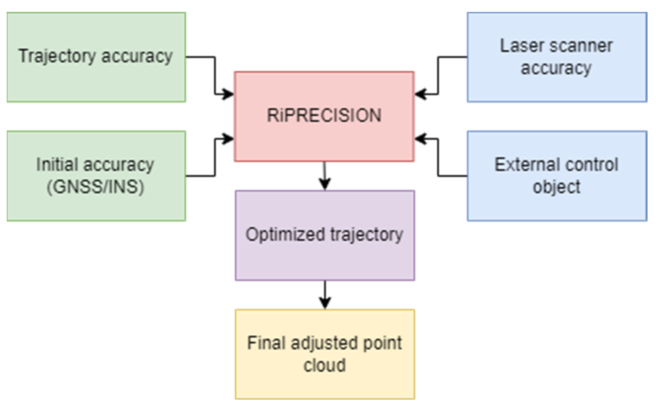
After marking the control points in individual clouds, the adjustment is followed by the RiPRECISION tool, whose possible inputs are described in Figure 4. The software allows three different alignments: non-rigid with translation (global shift with local alignment), non-rigid (local alignment), and rigid (global shift). In this project, a non-rigid with translation alignment was chosen. The tool takes all the input data, uses them to adjust and recalculate the initial trajectory, and as a final step, computes new point clouds based on the new trajectory. In the case of multiple data on a single path, it can merge the data into a single point cloud [33].

2.7. MLS Accuracy Evaluation

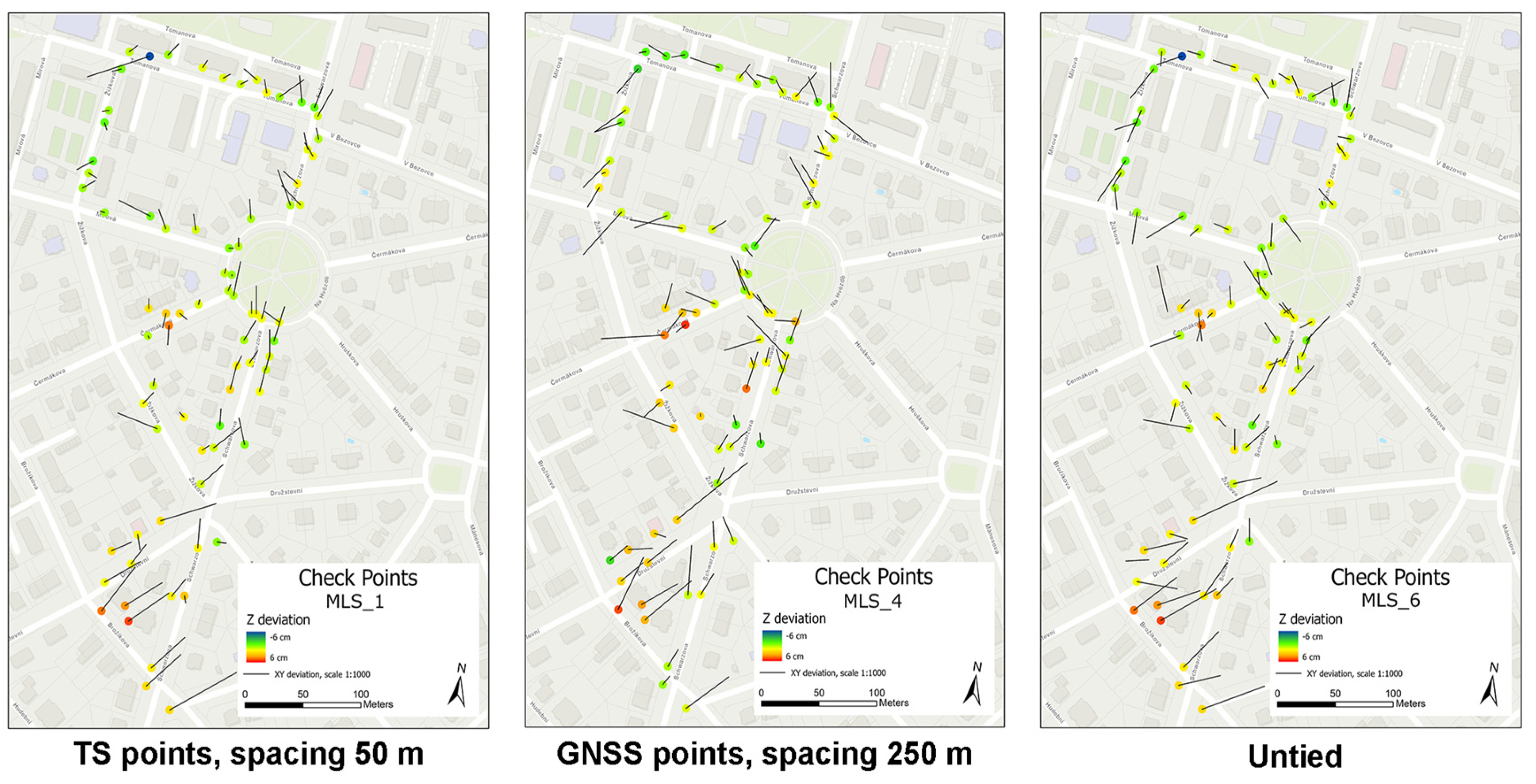
The accuracy evaluation was performed using two separate approaches. The first approach evaluates the accuracy of the points taken from the computed point clouds to the check points targeted by the total station from the adjusted point network [25,28]. In the second part, the computed point clouds are compared against each other [24,26,34].

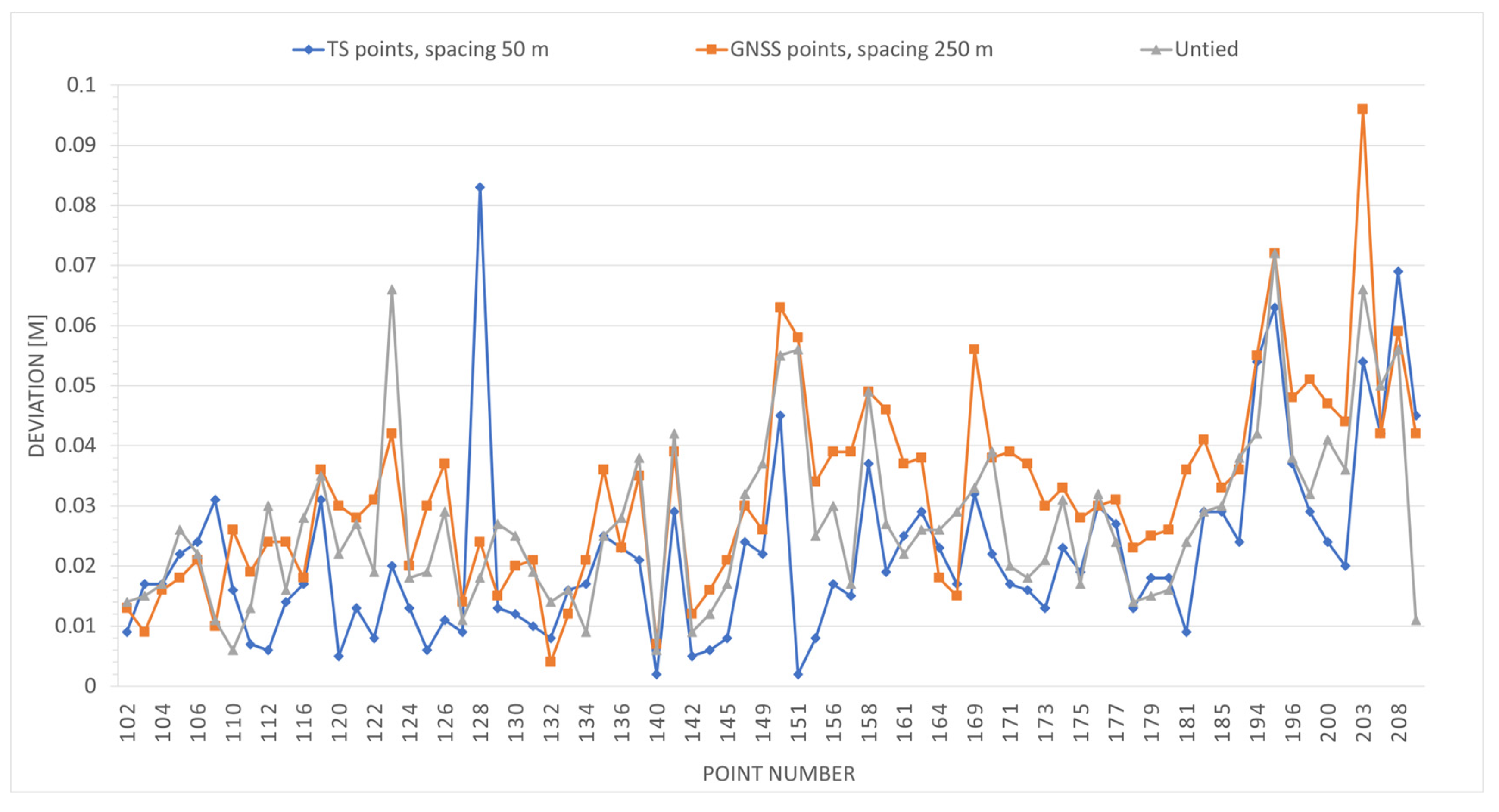
2.7.1. Comparison with Checkpoints

Custom software was developed to compare point clouds and measured checkpoints with higher accuracy, calculate deviations, and visualise them. It allows working in the European Terrestrial Reference System 89 (ETRS89) and in the System of the Unified Trigonometrical Cadastral Network (S-JTSK) together with the heights given in the Bpv system (Baltic Vertical after Adjustment). Since the measurements were carried out on the territory of the Czech Republic, S-JTSK and Bpv were chosen as the main coordinate systems of the results.

The developed software allows the calculation of coordinate differences, coordinate standard deviations (Equation (2)), root mean square deviations (Equation (1)), visualisation of these values in bar charts, and visualisation of deviations depending on the distance of the control points.

$$\mathrm{R}\mathrm{M}\mathrm{S}=\sqrt{\frac{{\sum }_{i=1}^n{\Delta x}_i^2}{n}},$$

(1)

where ${\Delta x}_i=X_i-{\widehat{X}}_i$, $X_i$ are the coordinates of the check point, ${\widehat{X}}_i$ are the coordinates of the point obtained from the point cloud.

$$\mathrm{S}\mathrm{t}\mathrm{D}\mathrm{e}\mathrm{v}=\sqrt{\frac{{\sum }_{i=1}^n{v}_i^2}{n-1}},$$

(2)

where $v_i=\Delta \overline{X}-{\Delta X}_i$, ${\Delta X}_i$ are the coordinators differences between the check points and the points obtained from the cloud, $\Delta \overline{X}$ is their average.

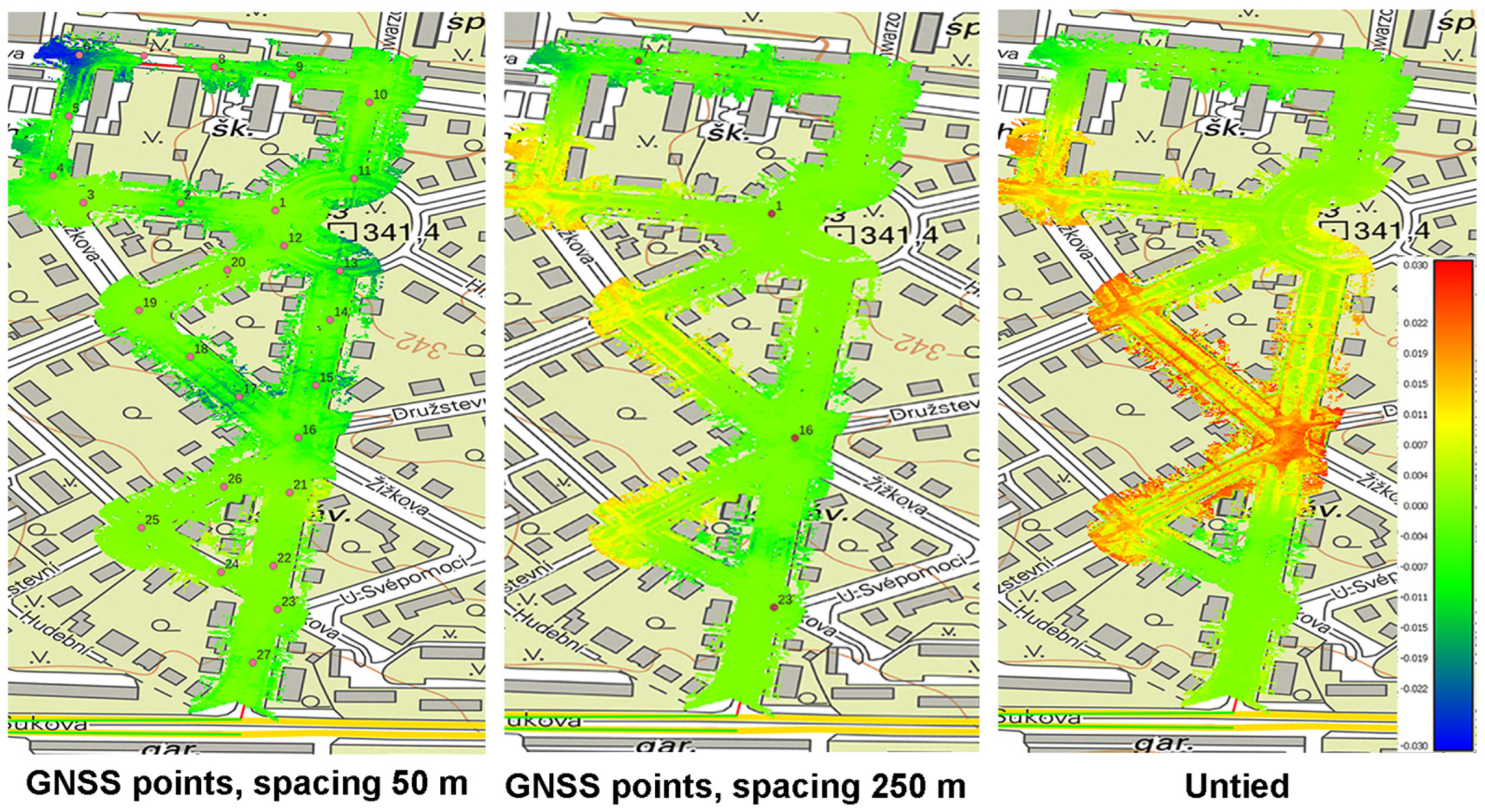
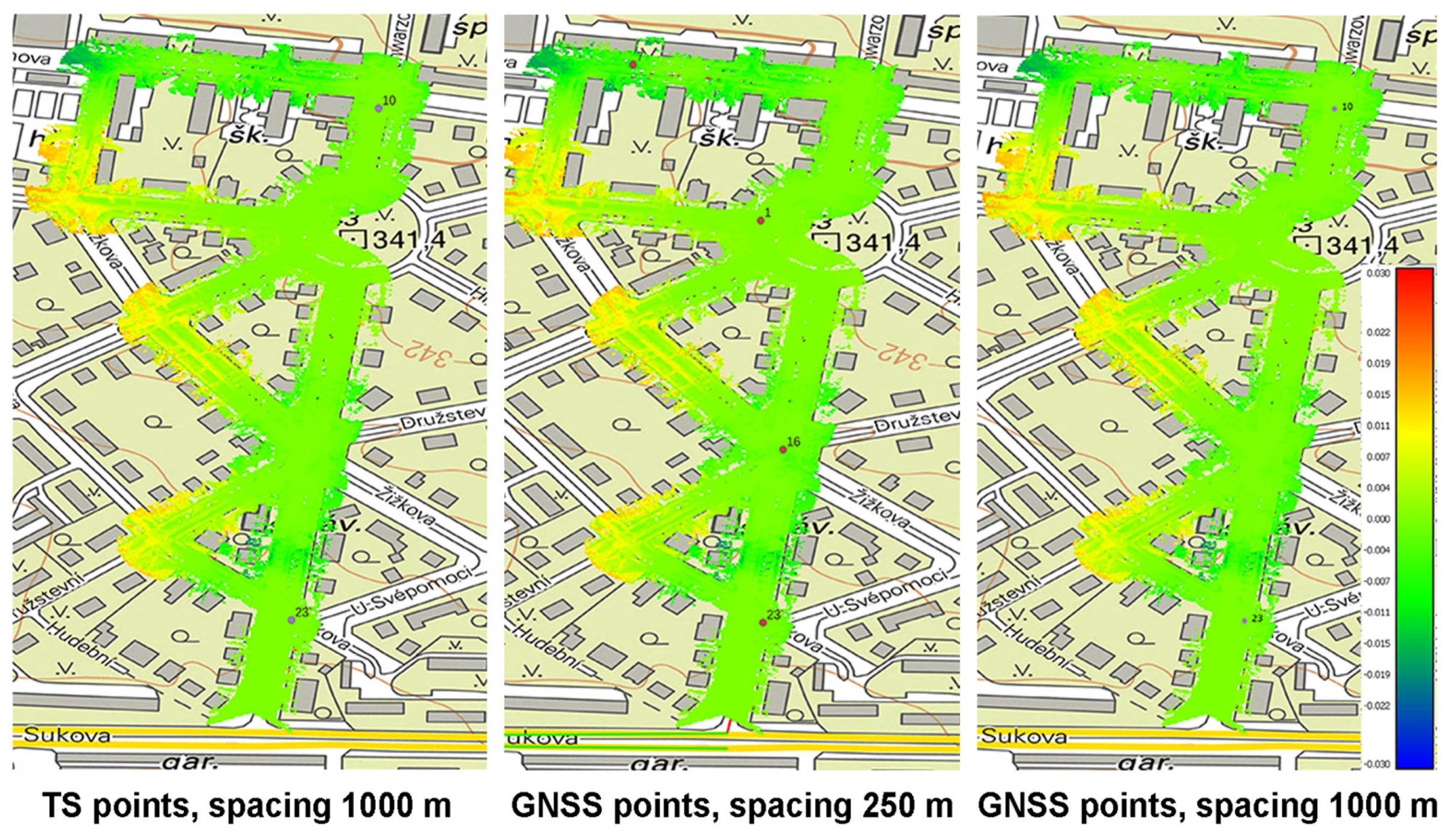
2.7.2. Comparison of Computed Clouds

To further analyse the behaviour of the clouds depending on the number and location of the control points, the computed clouds were compared with each other in CloudCompare software (https://www.danielgm.net/cc/).

As distinct from the previous case, the deviations are not related to the checkpoints but are calculated from the differences of all points from point clouds.

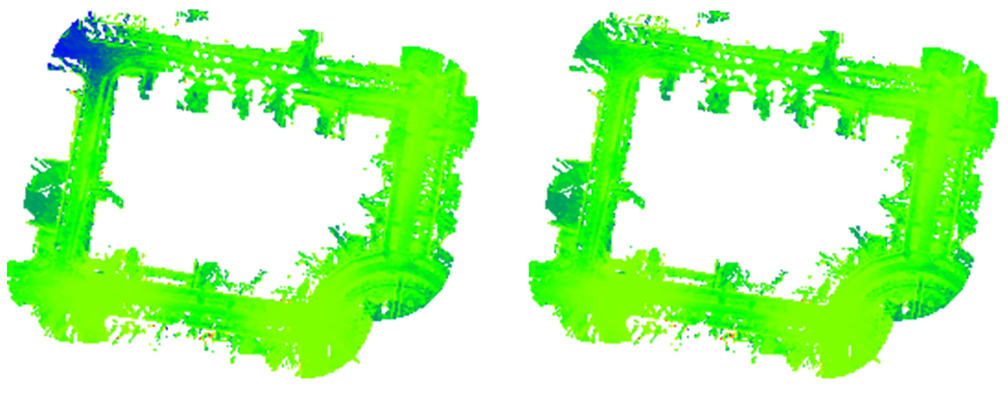
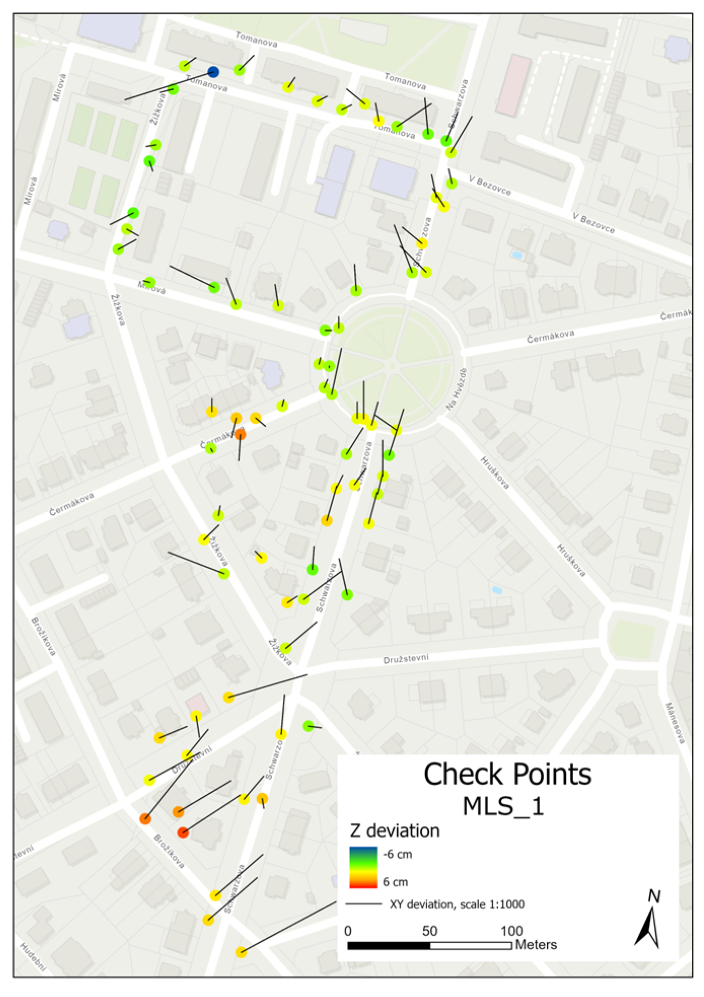
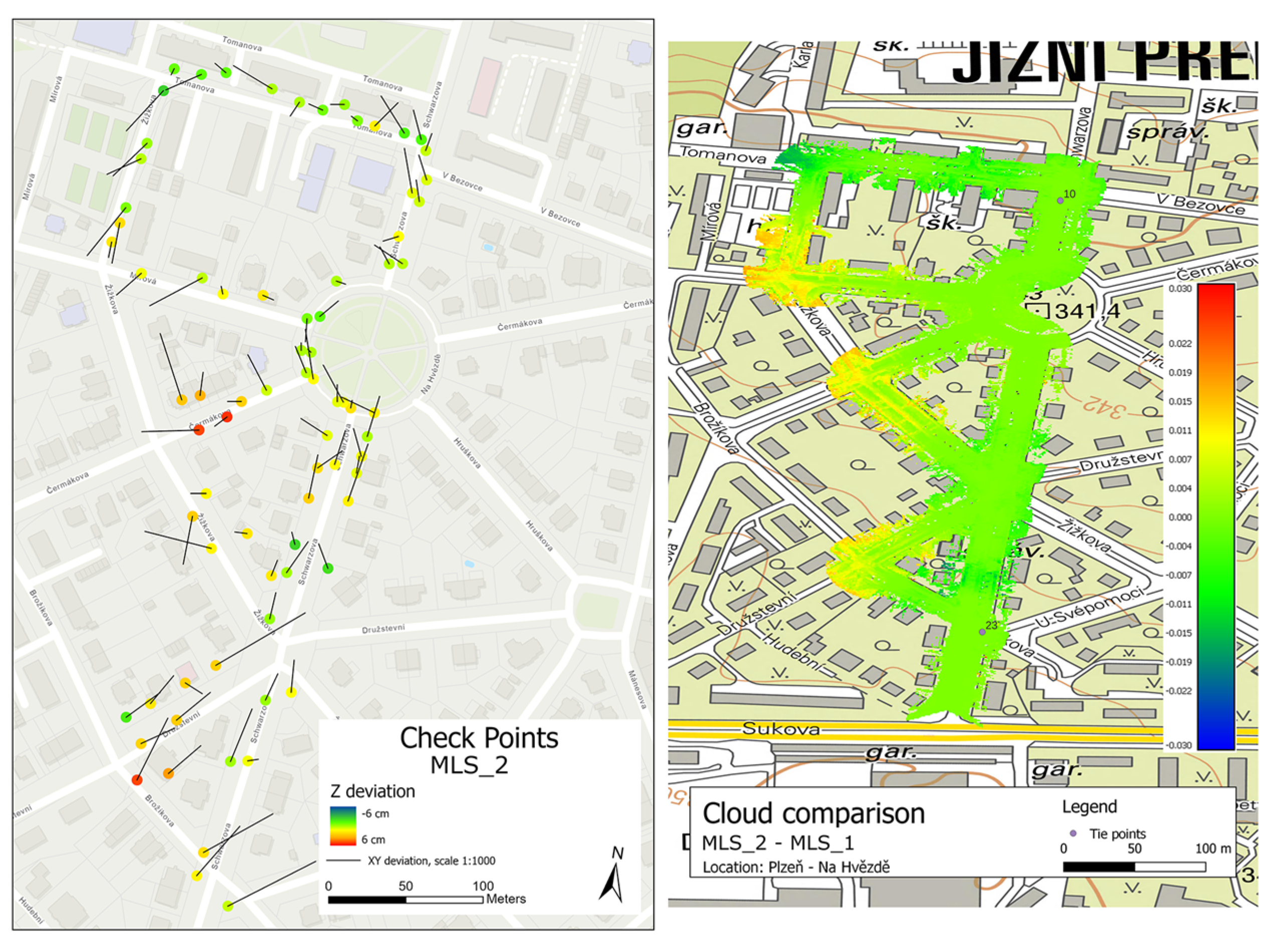
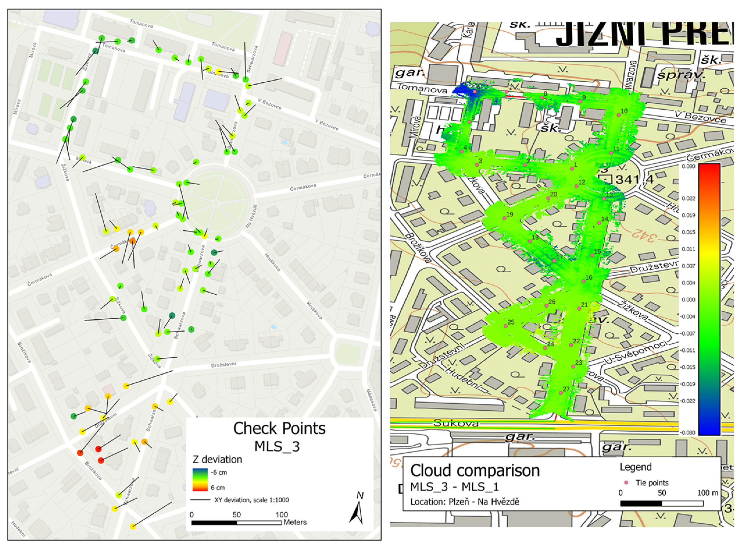
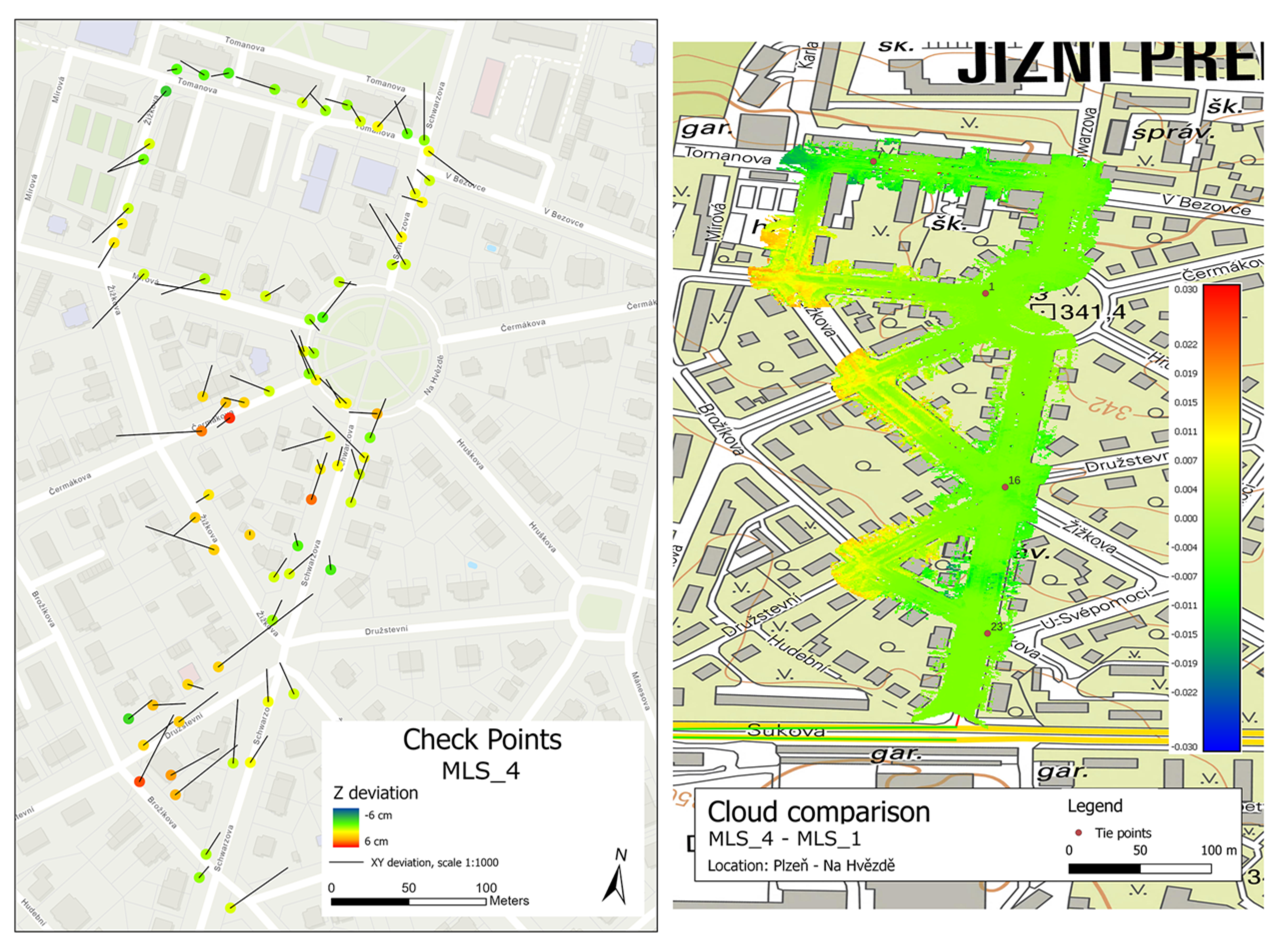
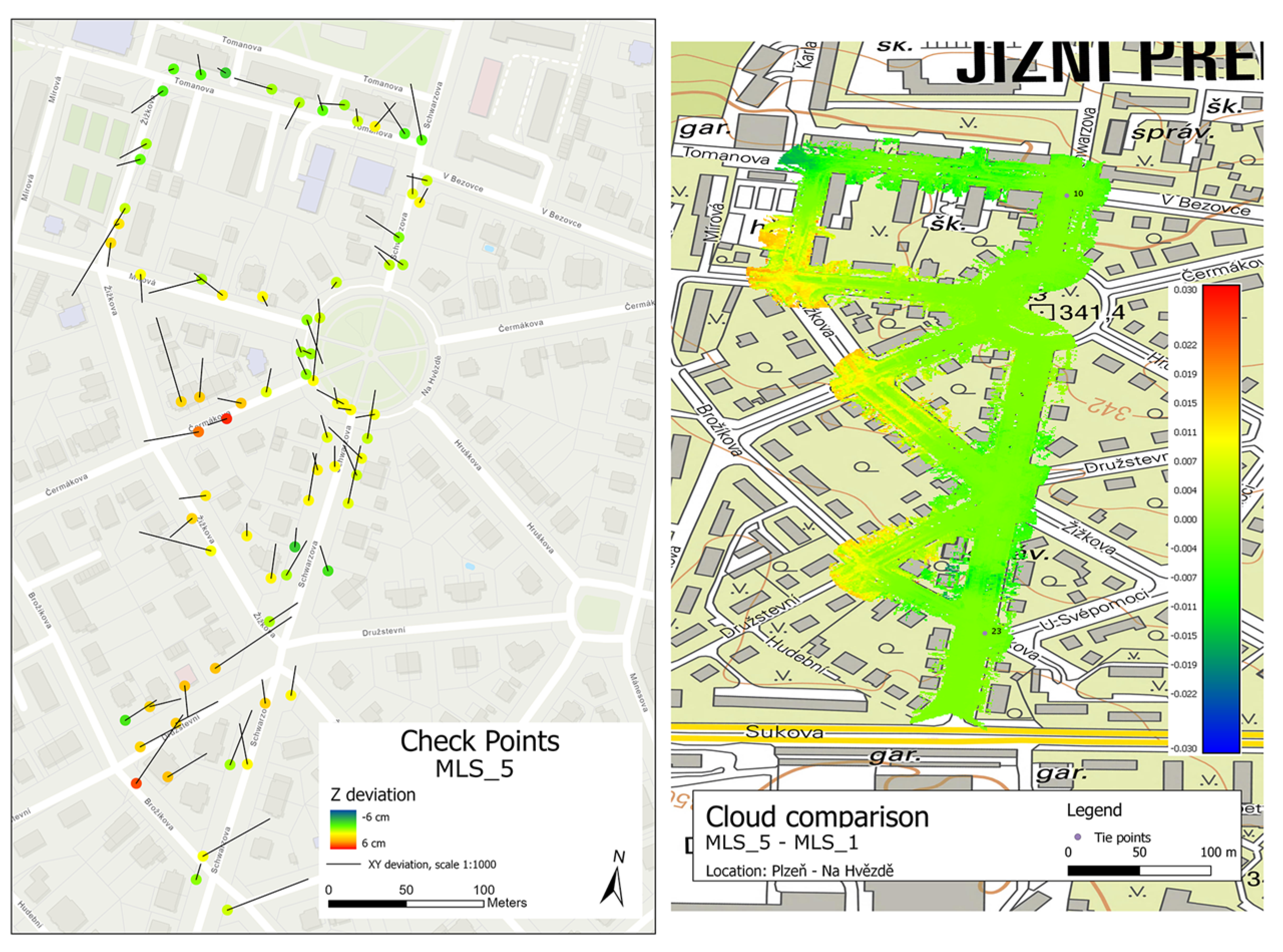
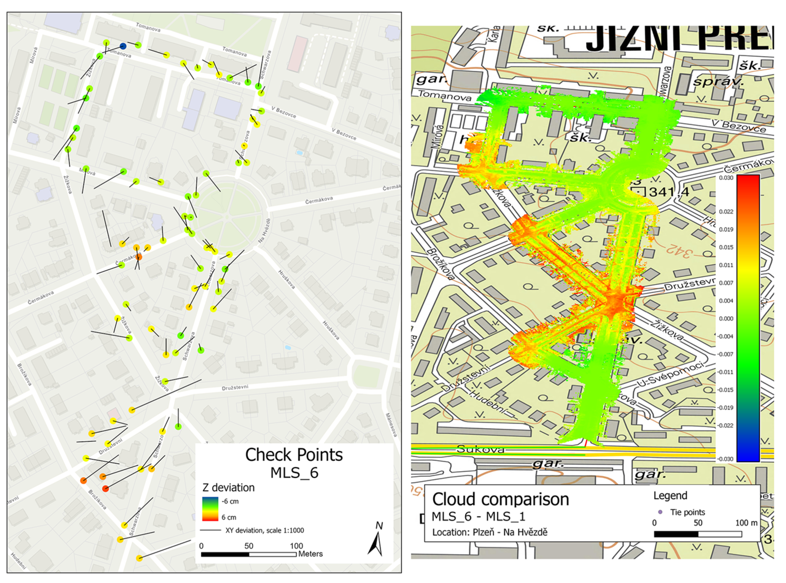
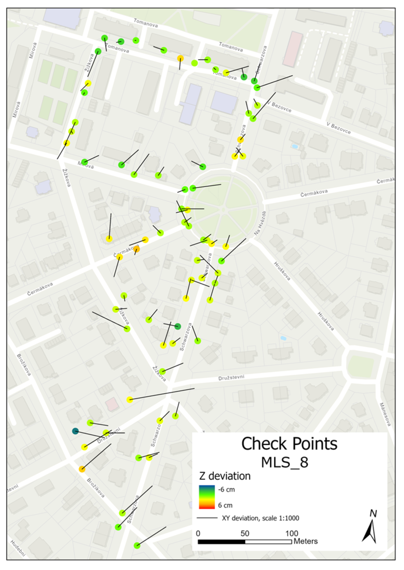
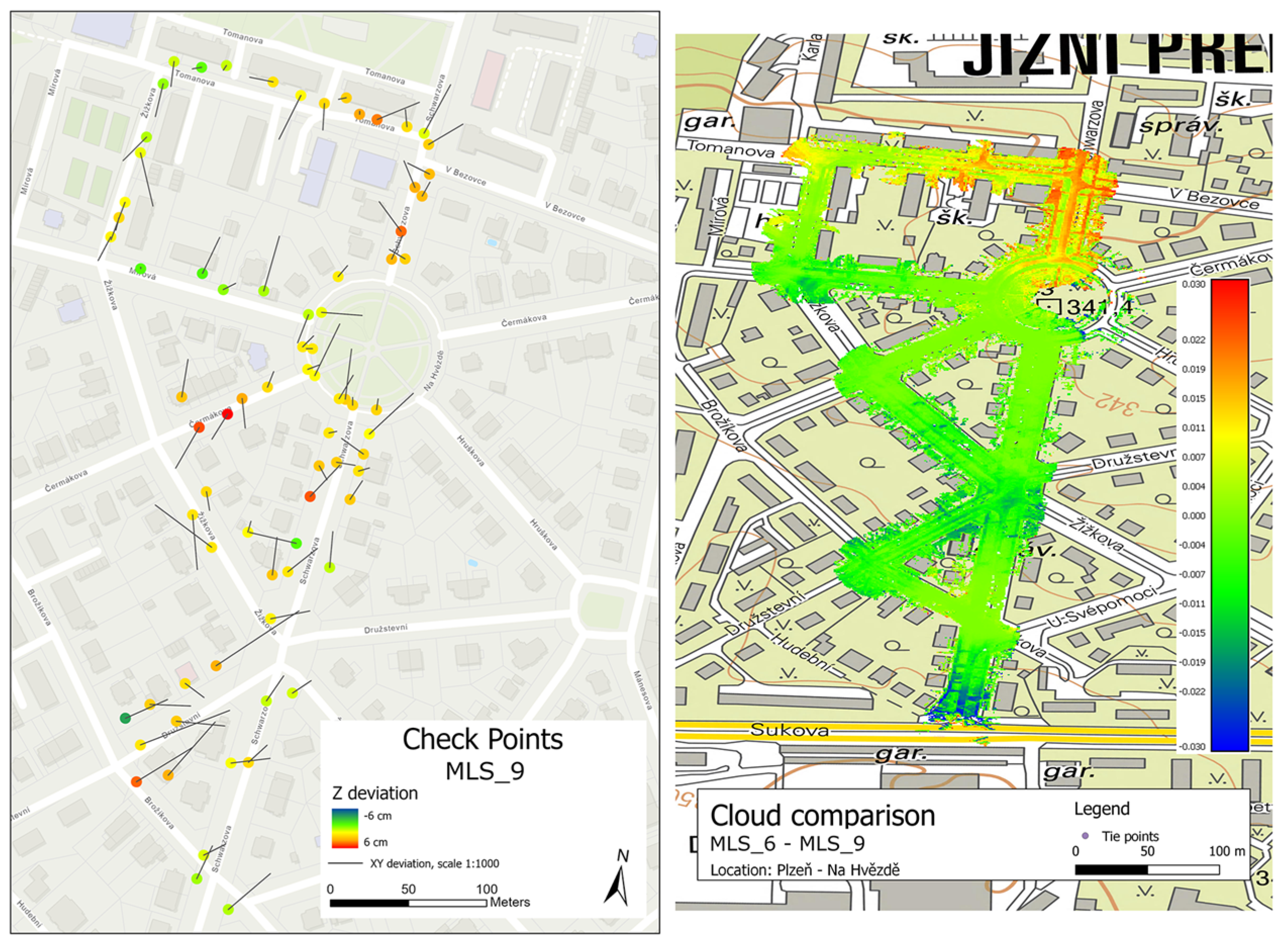
In the first phase, the point clouds were compared with the MLS_1 cloud, which was expected to be the most accurate. In the next phases, point clouds of different settings, which were expected to show interesting results, were compared. The outputs of this comparison are the average deviations of the compared clouds, a histogram of the cloud differences in the Z-axis direction, and a map showing the cloud differences and the control points in the map.

3. Results

In this part of the paper, the results are presented in the form of tables, graphs, and maps. The evaluation of the accuracy of the GNSS control points is presented first, revealing their effectiveness compared to total station (TS) measurements. Following this, the accuracy of point clouds is assessed through two approaches: comparison with TS checkpoints and comparison between different point cloud data sets. The results of the cloud evaluation are presented in summary tables. As an example, results from different point strategies are presented here. All results are found in the Appendix A.

3.1. Evaluation of the Accuracy of GNSS Control Points

In many cases, the GNSS RTK method is much faster than the total station measurements. However, the chapter “Test field specifications” shows that their accuracy is less than that of TS points.

Table 9. Accuracy evaluation of GNSS control points.

Coordinate	StDev [mm]	RMS [mm]
XY	14	20
XYZ	17	25

shows the standard deviations calculated from the coordinate differences of the GNSS control points and TS control points. From these values, it can be predicted what effect the use of GNSS control points may have on the calculated point cloud.

3.2. Point Cloud Accuracy Evaluation

The accuracy of the point clouds was evaluated in two ways. First, the point cloud points taken were compared with measured TS checkpoints [25]. This includes calculating the deviations and displaying them on graphs and maps. In addition, the clouds were compared with each other, the spatial deviations were calculated, and a map of the point cloud differences was made [24,26].

3.2.1. Comparison with Checkpoints

From the differences between the coordinates of the check TS points and the coordinates of the points taken from the calculated point cloud, the deviations shown in

Table 10. Mean standard deviations and root mean square deviations of point clouds.

Point Cloud Name	Control-Point Specs	StDev XYZ [mm]	RMS XYZ [mm]
MLS_1	Adjusted (TS) 50 m	24	28
MLS_2	Adjusted (TS) 1000 m	29	31
MLS_3	GNSS RTK 50 m	32	32
MLS_4	GNSS RTK 250 m	30	33
MLS_5	GNSS RTK 1000 m	29	31
MLS_6	Untied	30	36
MLS_7	Adjusted (TS) 50 m	22	25
MLS_8	GNSS RTK 1000 m	25	26
MLS_9	Untied	28	35

were calculated. Maps (Figure 5) display the direction and magnitude of the deviations of the checkpoints taken from the point clouds. This visualisation may indicate possible local deformations in the point cloud. Figure 6 shows the deviations at the checkpoints along the data collection route.

3.2.2. Comparison to Other Clouds

To find point cloud deformations without dependence on checkpoints, point clouds were compared in CloudCompare software mostly with MLS_1, a point cloud tied on TS points with 50 m spacing. The smallest deviations were expected for this point cloud.

The 3D deviations were then calculated from the coordinate differences and are given in

Table 11. Point clouds difference comparison deviations from CloudCompare software.

Reference Cloud	Compared Cloud	StDev XYZ [mm]	RMS XYZ [mm]
MLS_1	MLS_2	3	3
MLS_1	MLS_3	5	6
MLS_1	MLS_4	3	4
MLS_1	MLS_5	3	3
MLS_1	MLS_6	7	9
MLS_6	MLS_9	8	8

. Figure 7 shows maps of clouds in comparison with MLS_1. These compared clouds have various spacing of control points. The maps show the deviations and visualise the cloud deformation. Figure 8 then shows a comparison of clouds with a different spiky strategy but with similar results.

4. Discussion

This work was concerned with determining the accuracy of mobile laser scanning in urban areas. A total of nine point clouds with different characteristics were made. Detailed analysis and comparisons were made to determine their properties and behaviour in specific areas.

4.1. MLS_1

The point cloud used adjusted control points measured by the total station with 50 m spacing shows some of the smallest deviations of all the point clouds evaluated. The average spatial standard deviation of the point cloud calculated from the differences between the checkpoints is 24 mm (

Table A1. Mean standard deviations and root mean square deviations of MLS_1.

Coordinate	StDev [mm]	RMS [mm]
X	11	15
Y	16	16
Z	15	17
XY	19	22
XYZ	24	28

). Most spatial differences are below 30 mm, but there are local variations that can be assigned to poorer point identification. In the part between points 23, 24, and 25 there are indications of systemic point cloud deformation in the horizontal direction (Figure A1). The largest spatial difference of the checkpoint is 60 mm, but this is an anomaly.

The work [25] worked with ground control points with the same spacing and quality as this experiment, but the resulting accuracy was higher. This may be due to the identification of checkpoints. This paper uses 3D spatial points as checkpoints [25] and uses very well-signalised points (embedded targets).

4.2. MLS_2

The point cloud tied by the TS points after 1000 m shows much larger deviations than MLS_1. This may be due to the software using only very accurate points in their surroundings and using GNSS/INS data for the rest of the route. Larger deviations are observed in the last part, indicating local point cloud deformation or poor point identification. The mean standard deviation of the cloud is 29 mm (

Table A2. Mean standard deviations and root mean square deviations of MLS_2.

Coordinate	StDev [mm]	RMS [mm]
X	16	19
Y	18	18
Z	16	18
XY	24	26
XYZ	29	31

).

From Figure A2 can be seen that the deviation values are around zero, with only three locations showing a degraded accuracy. In these locations, the car carrier drove out from a spot where the view of the sky was obscured, and then the car was turned.

4.3. MLS_3

The point cloud tied with GNSS points after 50 m shows a larger influence of the lower quality points on the whole point cloud, especially in the vertical direction. The average standard deviation of the point cloud is 32 mm (

Table A3. Mean standard deviations and root mean square deviations of MLS_3.

Coordinate	StDev [mm]	RMS [mm]
X	18	18
Y	17	17
Z	20	20
XY	25	25
XYZ	32	32

). Spatial differences are, in most cases, below 50 mm (Figure A3). The largest spatial difference of the checkpoint is 65 mm. Figure 9, on the left, shows the local cloud deformation due to the use of a poor-quality GNSS control point. On the right is the calculated cloud without the control point 6.

4.4. MLS_4

The point cloud tied with GNSS points after 250 m has slightly worse accuracy than MLS_2. Its properties are similar. At greater distances from the control points, local deformations are observed, mainly due to obscuration of the sky view by trees (Figure A4). The average standard deviation of the point cloud is 30 mm (

Table A4. Mean standard deviations and root mean square deviations of MLS_4.

Coordinate	StDev [mm]	RMS [mm]
X	16	18
Y	20	20
Z	16	19
XY	26	27
XYZ	30	33

). The largest spatial difference of the checkpoint is 81 mm, but this is an isolated value; the other spatial differences are below 60 mm. The comparison in Figure A4 with the MLS_1 point cloud shows that in sharp turns and in areas where the view is obscured, deformations occur.

The paper [26] gives a 2D accuracy of about 2 cm for similar point spacing. Although this work was performed under different conditions, the results are very similar.

4.5. MLS_5

Table A5. Mean standard deviations and root mean square deviations of MLS_5.

Coordinate	StDev [mm]	RMS [mm]
X	17	19
Y	17	17
Z	16	18
XY	24	26
XYZ	29	31

and Figure A5 show that the point cloud using GNSS control points with a spacing of 1000 m has the same properties as the point cloud using GNSS control points with a spacing of 250 m (MLS_4).

4.6. MLS_6

The untied point cloud shows the same average deviation as the MLS_4 tied point cloud, which is 30 mm (

Table A6. Mean standard deviations and root mean square deviations of MLS_6.

Coordinate	StDev [mm]	RMS [mm]
X	16	16
Y	19	20
Z	17	26
XY	25	26
XYZ	30	36

). The spatial differences are below 65 mm (Figure A6). The largest spatial difference of the checkpoint is 97 mm, but this is an isolated value.

By comparing the point clouds, it is easy to see the segments where there is more tree cover and, therefore, a degradation in the accuracy of the GNSS receiver. The average standard deviation of the difference between the point clouds is significantly larger than the other clouds, 7 mm.

4.7. MLS_7

The average spatial standard deviation of the point cloud from the second data collection using TS points with 50 m spacing is 22 mm (

Table A7. Mean standard deviations and root mean square deviations of MLS_7.

Coordinate	StDev [mm]	RMS [mm]
X	13	16
Y	13	13
Z	12	13
XY	18	21
XYZ	22	25

). This point cloud has similar properties to the point cloud from the first data collection (MLS_1); it can be seen that some of the larger deviations from the MLS_1 cloud were random and the systematic error in parts 23 to 25 was confirmed (Figure A7).

The difference in standard deviations of the MLS_7 and MLS_1 data sets (two independent sections with the same properties) is 2 mm; this value of cloud difference is very similar to the results of [24].

4.8. MLS_8

The point cloud using GNSS control points with a spacing of 1000 m from the second data collection, even considering MLS_7, shows that the second data collection was better in the case of accuracy. The average spatial standard deviation of the cloud is 25 mm (

Table A8. Mean standard deviations and root mean square deviations of MLS_8.

Coordinate	StDev [mm]	RMS [mm]
X	12	14
Y	17	17
Z	14	14
XY	11	22
XYZ	25	26

). Most spatial differences are below 40 mm (Figure A8).

4.9. MLS_9

The standard deviations of Untied clouds from both data collections are very similar (Table A6 and

Table A9. Mean standard deviations and root mean square deviations of MLS_9.

Coordinate	StDev [mm]	RMS [mm]
X	17	17
Y	16	17
Z	16	24
XY	23	25
XYZ	28	35

). By comparing the untied point clouds from the first and second data collections (Figure A9), it can be observed that their behaviours are also very similar. The exceptions are the sections where the first data collection started, the second ended, and the other way around. The average standard deviation of the difference between point clouds is 8 mm.

5. Conclusions

Mobile mapping, a method used in surveying, faces various factors that can influence its accuracy and efficiency.

The first presumed negative influence is the speed of data collection. In this work, two data collections were made with different speeds of 20 and 35 km/h. The analysis shows that higher speed, and therefore lower point cloud density, does not have a degrading effect on the accuracy of the resulting point cloud. Data collection at higher speed results in an average 2 mm better StDev XYZ.

The second expected factor that affected the accuracy of the result is the configuration and quality of the control/tie points. The influence of control point spacing on the overall cloud accuracy was confirmed from only one comparison, that between a cloud with TS points spaced 50 m apart and a cloud with TS points spaced 1000 m apart. The StDev XYZ for a cloud with a point spacing of 50 m is 24 mm and 29 mm for a point spacing of 1000 m. However, for clouds from the first data collection tied to GNSS points, StDev XYZ is around 30 mm, independent of the spacing of the control points. From the maps, locations where local cloud deformations occur were identified; these are sharp turns when leaving a location with a poorer view of the sky and larger distances from the control points. This deviation can be minimised in most cases by the appropriate location of the control point.

However, the influence of the quality of the points plays an important role. MLS_3 point clouds tied using a GNSS point with 50 m spacing show worse deviations than point clouds with larger spacing. This was due to the less accurate determination of the control points at locations with an obscured sky view and therefore a degradation of the quality of the GNSS RTK measurements. The results suggest that it is appropriate to select spots where the positioning of the control point will not be affected by negative influences, even at the cost of larger point spacings.

The overall quality of the result can also be influenced by the ability to identify the point. Points signalled by chequerboard targets or street lines can be identified with a repeatability of 4 mm and spatial features with a repeatability of 9 mm. This error is particularly visible in the last part of the tested section, where checkpoints were harder to identify.

This project has demonstrated that the highest measurement accuracy in urban areas can be achieved by using high-precision control points spaced at 50 m. Here, points with an average XYZ standard deviation of 2.2 mm were used. In this case, an average point cloud standard deviation of 22 mm was achieved. However, the making of such an accurate network is very time- and cost-consuming and in real terms inefficient and uneconomical.

Using GNSS grid points, the point cloud accuracy, independent of the spacing of the grid points, was around 30 mm.

In conclusion, even in the less ideal conditions in this project, the accuracy achieved in urban areas was better than or equal to the manufacturer’s stated GNSS/INS positioning accuracy for ideal conditions. From the comparison of the calculated GNSS RTK checkpoint deviations and the MLS checkpoint deviations, it can be said that the mobile laser scanning method in urban areas is more accurate than the GNSS RTK method. For the above reasons, the mobile mapping method using the RIEGL VMX-2HA system can replace GNSS measurements in urban areas to a large extent. This will speed up the measurements, save costs since a trained surveyor will not be needed to collect the data, ensure the measured data will be more detailed and wider, and ensure more information can be obtained not only about the objects of interest but also their surroundings.

Despite the insights gained from this study, certain limitations must be acknowledged. This study focused on the accuracy of one type of mobile mapping device used for mapping urban build-up areas. Data collection was carried out under specific weather conditions, which can affect the results.

Further research in different environments, under different weather conditions, could provide more comprehensive insights for data collection by mobile mapping systems. The method of mobile scanning by vehicle could become one of the main methods of modern mapping in the near future. In combination with aerial scanning, drone scanning, and handheld mobile scanning, detailed measurements of even large areas could be made in a relatively short time. It would also find great use in more demanding methods such as road condition inspection or surveying and checking road layers and slopes during construction. This is not yet possible with the VMX-2HA in the configurations shown; further research could be focused on technological solutions to this issue.