

Position-Based Formation Control Scheme for Crowds Using Short Range Distance (SRD)


Abstract
:1. Introduction
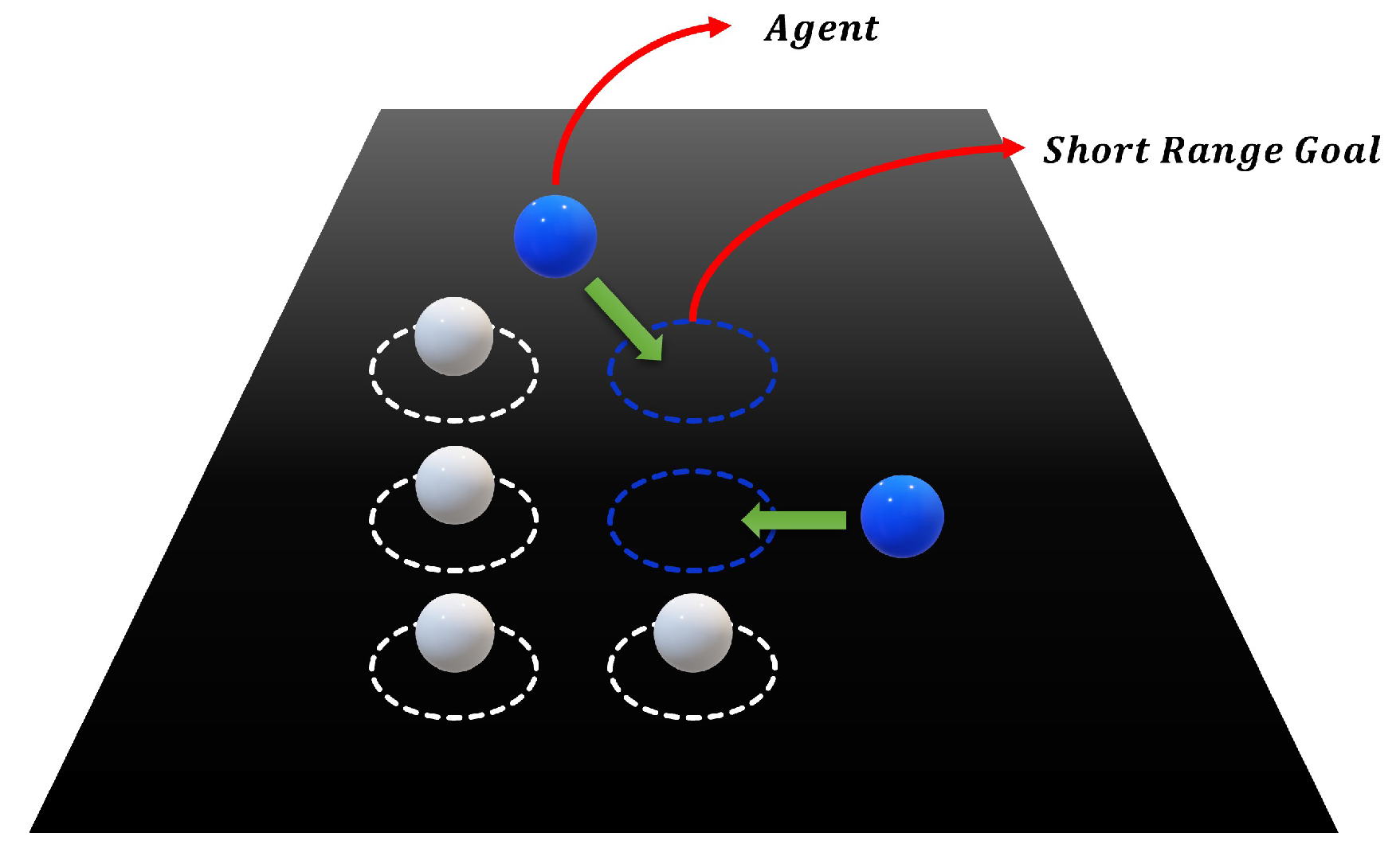
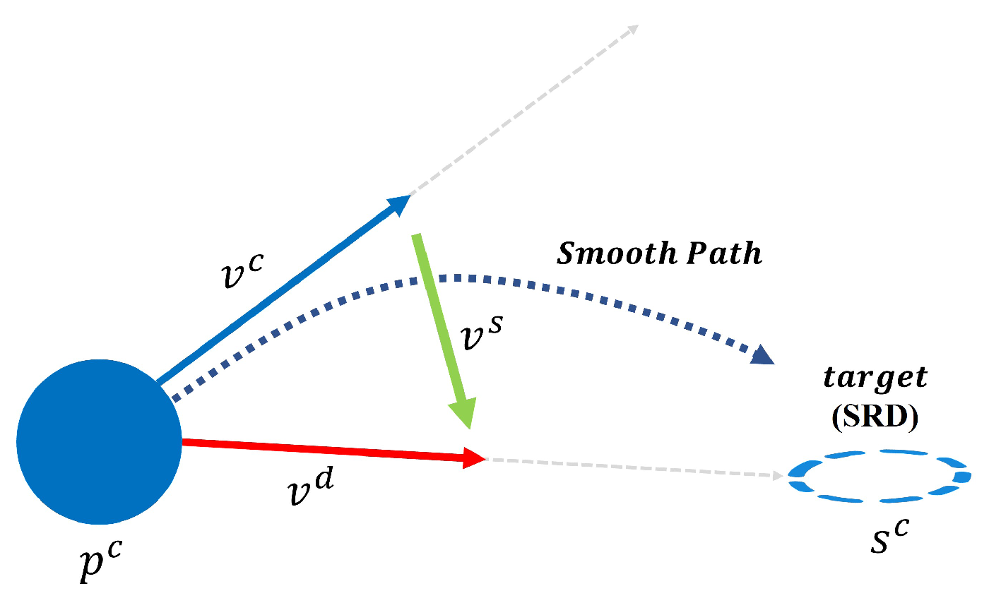
- We propose a new algorithm that introduces a scheme called Short Range Destination (SRD) to help crowds move to a destination while satisfying a given shape;
- We propose a method of leveling constraints that allows the agent to determine for itself which constraints it should respond to in various situations;
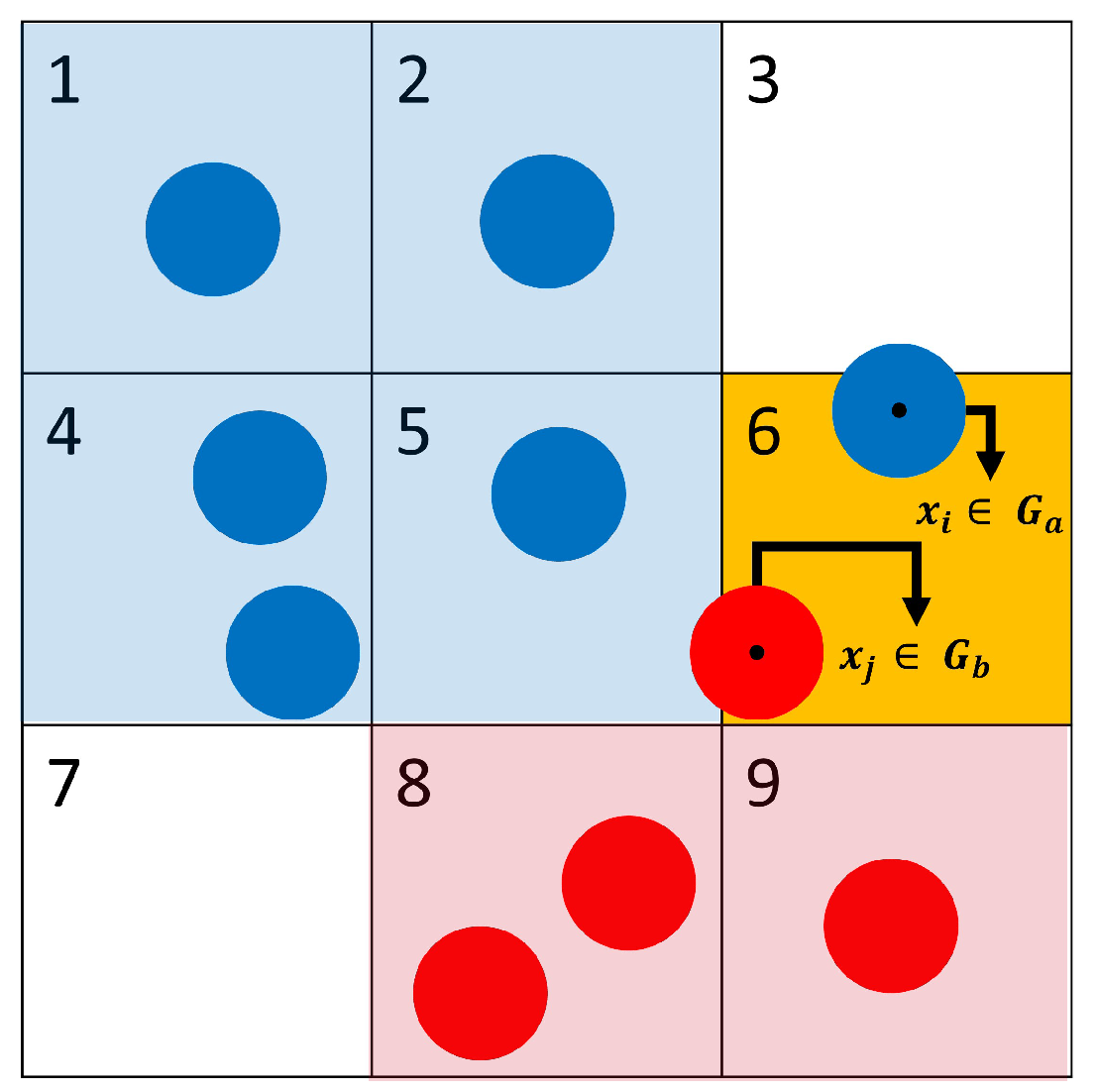
- Our method grids the field in two dimensions and embeds local information, which is combined with the respective leveled constraints to influence the decisions of each agent.
2. Related Work
2.1. Crowd Simulation
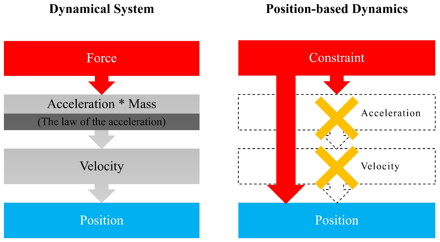
2.2. Dynamical Systems and PBD
2.3. Crowd Formation Control Methods
3. Proposed Algorithms
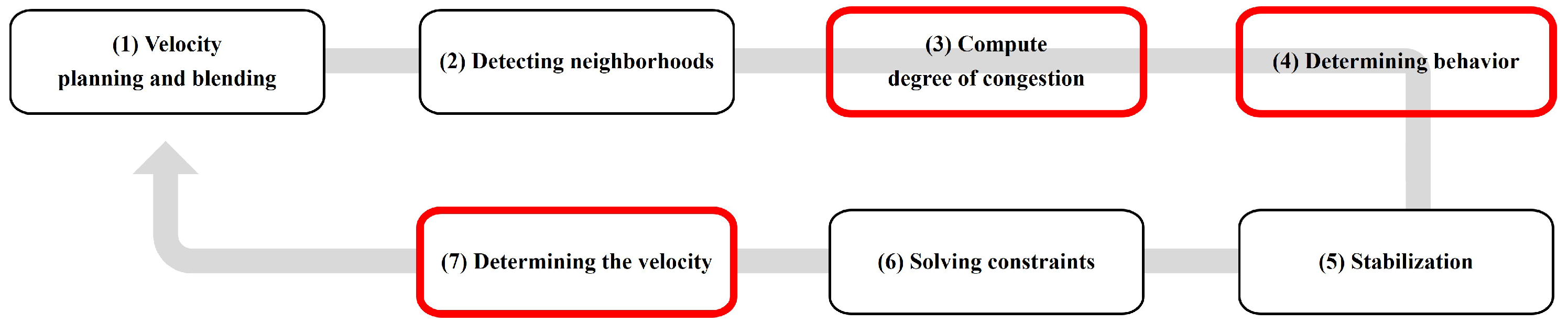
3.1. Overview
- 1.
- Velocity planning and blending: Given a planned velocity that leads the agent to the final destination, each agent blends the current velocity with the planned velocity together. Then, the future position is predicted from the blended velocity;
- 2.
- Detecting neighborhoods: This step updates the local information. It includes the presence or absence of agents in neighboring spaces, the number of neighboring agents, and the number of agents belonging to other groups. Each agent can detect neighborhoods using this local information;
- 3.
- Computing the degree of congestion: This step uses the local information explored in the previous step. The degree of congestion calculated with the local information is then mapped onto the grid space;
- 4.
- Determining behavior: In this step, the soft constraints, such as the formation constraint, are enforced. After that, the agent determines whether to follow the soft constraints or not;
- 5.
- Stabilization: Since agents are rigid bodies, interpenetration is not allowed. In this step, hard constraints are enforced so that neighboring agents are repositioned to prevent them from being penetrated by each other;
- 6.
- Solving constraints: This is a step to solve the constraints. Constraints are set to control the distance between neighboring agents and avoid obstacles in the previous steps. At this stage, it predicts the future position after solving the constraints;
- 7.
- Determining the velocity: The velocity is derived from the difference between the predicted future position and the current position in the constraint-solving step. The speed limit of the agent is set in advance to increase stability. Furthermore, this method applies the steering behavior technique to prevent sudden changes in the velocity of agents when moving along the path [14]. Through these processes, the agent is moved by the final velocity.
| Algorithm 1 Crowd formation control using SRD |
|
3.2. Setup for User-Specific Environment
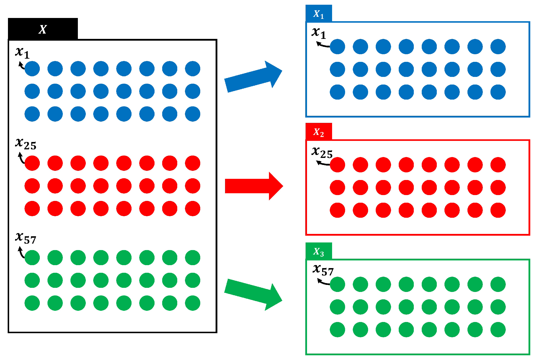
3.2.1. Crowds, Groups, and Agents
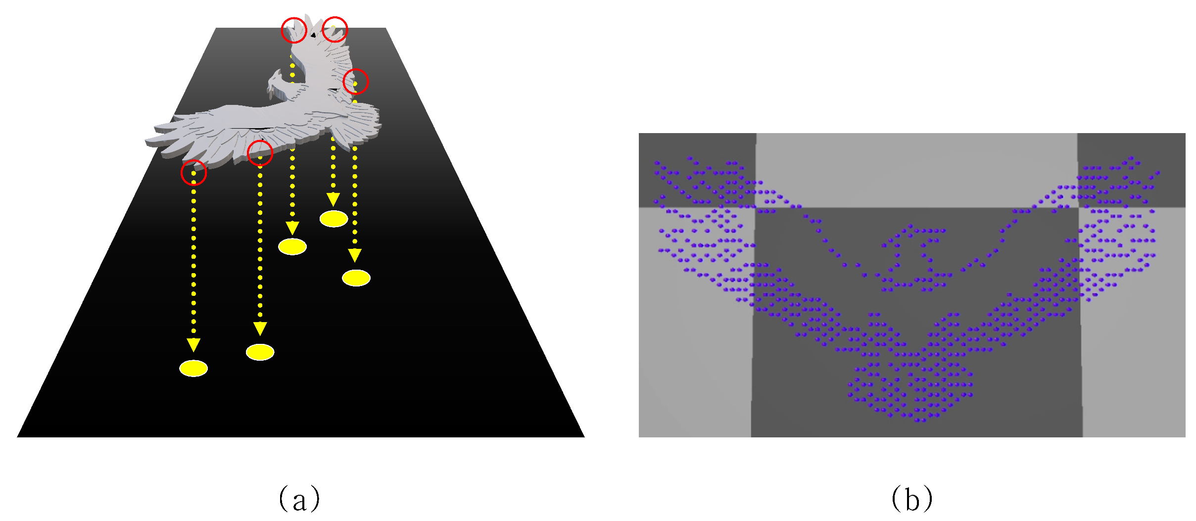
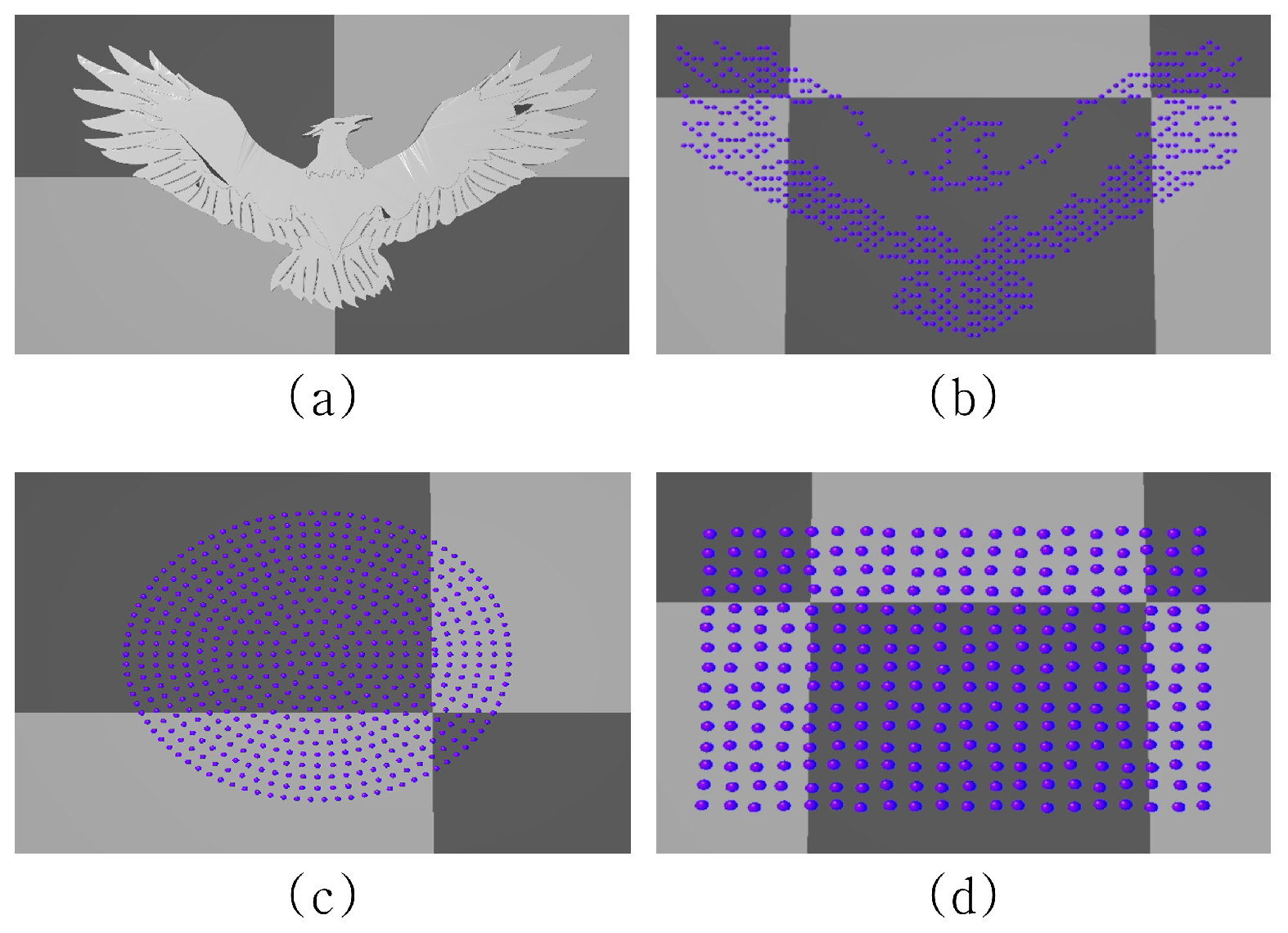
3.2.2. Crowd Formation Constraint: Forced Position Constraints for Agents
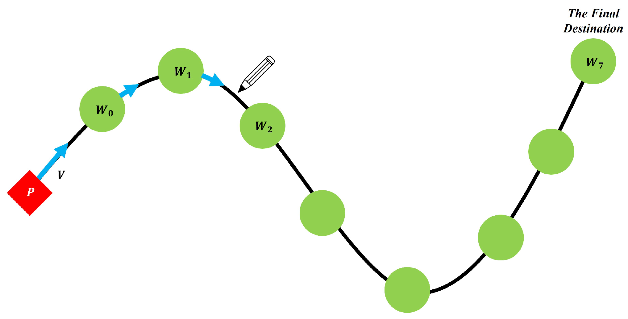
3.2.3. User-Drawn Group Path
3.3. Proposed Algorithms
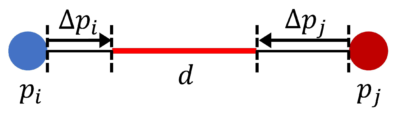
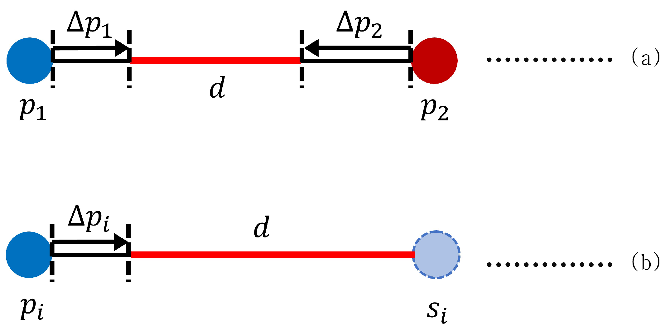
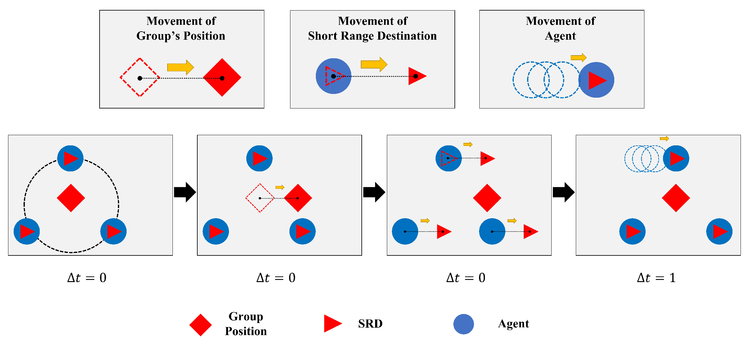
3.3.1. Short Range Destination (SRD)
3.3.2. Degree of Congestion
3.3.3. Steering Behavior for Control Inertia
4. Experiments
- CPU: Intel i7-8700 with 32 G main memory;
- GPU: NVIDIA RTX3080;
- IDE: Visual Studio 2019;
- Graphic Library: OpenGL 4.3.
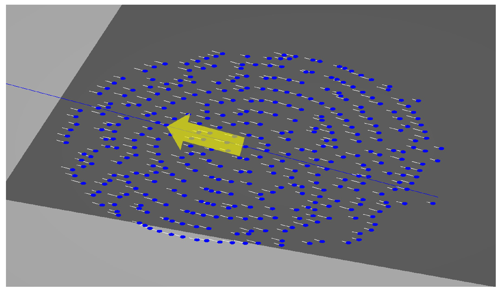
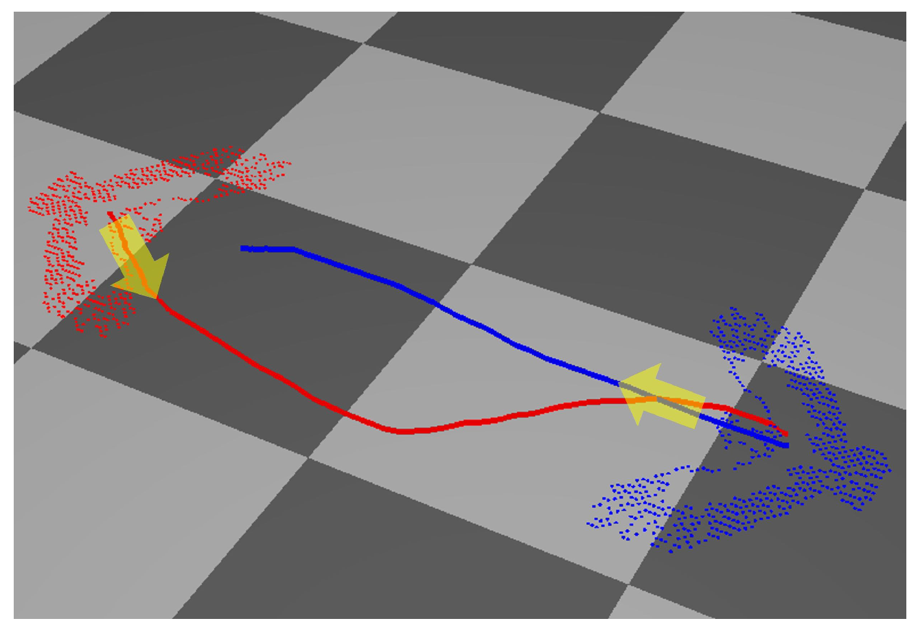
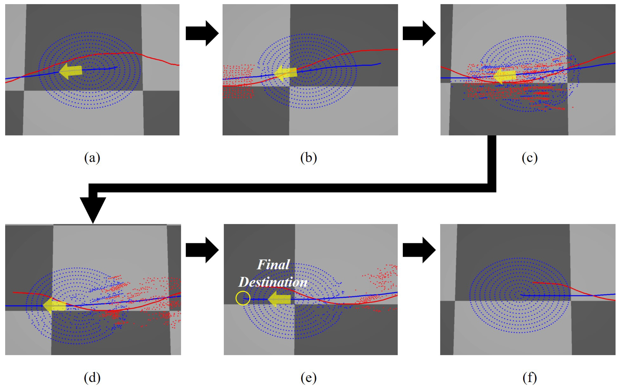
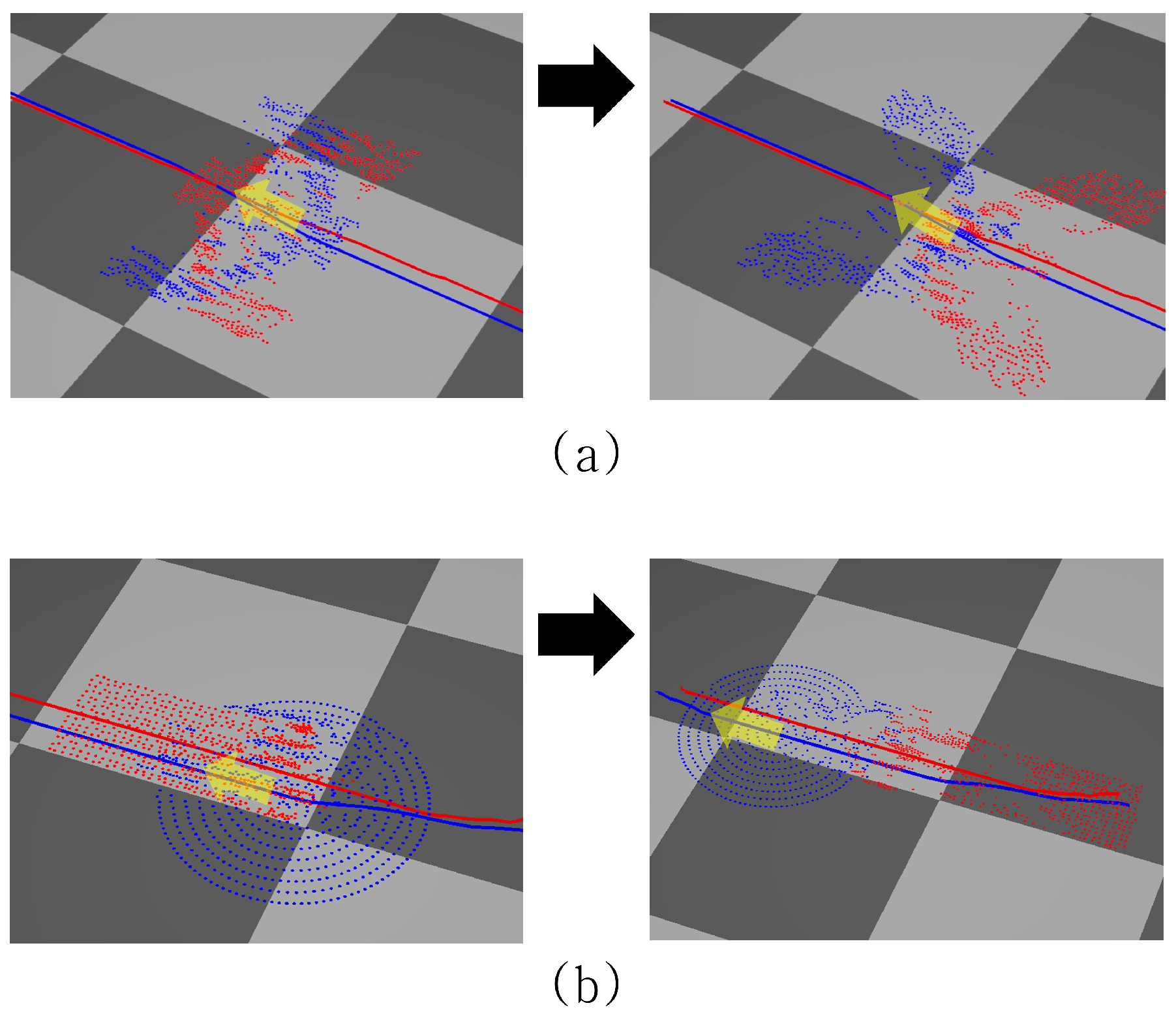
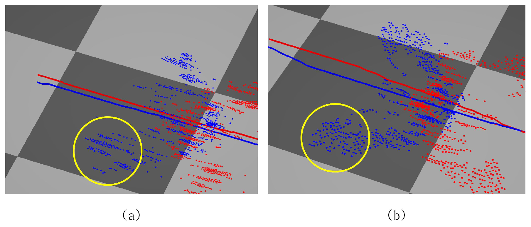
4.1. Formation Control on a Dynamic Environment
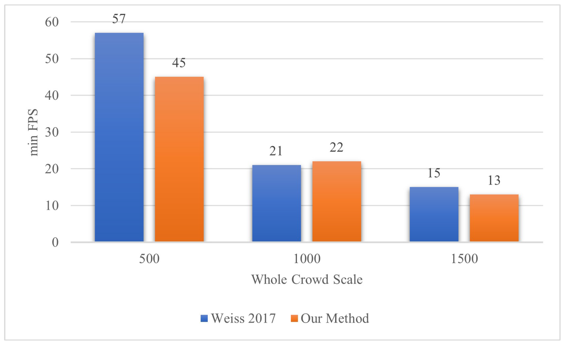
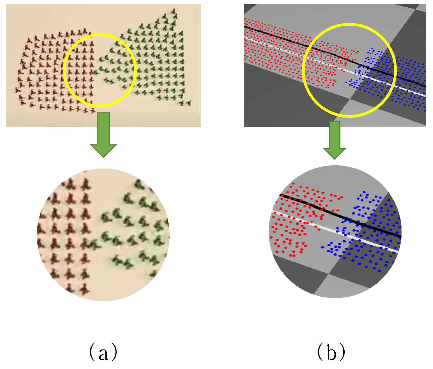
4.2. Comparison with Other Methods
5. Conclusions
Supplementary Materials
Author Contributions
Funding
Institutional Review Board Statement
Informed Consent Statement
Data Availability Statement
Conflicts of Interest
References
- Xu, M.; Wu, Y.; Ye, Y.; Farkas, I.; Jiang, H.; Deng, Z. Collective crowd formation transform with mutual information–based runtime feedback. Comput. Graph. Forum 2015, 34, 60–73. [Google Scholar] [CrossRef]
- Treuille, A.; Cooper, S.; Popović, Z. Continuum crowds. ACM Trans. Graph. (TOG) 2006, 25, 1160–1168. [Google Scholar] [CrossRef]
- Narain, R.; Golas, A.; Curtis, S.; Lin, M.C. Aggregate dynamics for dense crowd simulation. In Proceedings of the ACM SIGGRAPH Asia 2009 Papers, Yokohama, Japan, 16–19 December 2009; pp. 1–8. [Google Scholar]
- Weiss, T.; Litteneker, A.; Jiang, C.; Terzopoulos, D. Position-based multi-agent dynamics for real-time crowd simulation. In Proceedings of the ACM SIGGRAPH/Eurographics Symposium on Computer Animation, Los Angeles, CA, USA, 28–30 July 2017; pp. 1–2. [Google Scholar]
- Karamouzas, I.; Skinner, B.; Guy, S.J. Universal power law governing pedestrian interactions. Phys. Rev. Lett. 2014, 113, 238701. [Google Scholar] [CrossRef] [PubMed]
- Hesham, O.; Wainer, G. Advanced models for centroidal particle dynamics: Short-range collision avoidance in dense crowds. Simulation 2021, 97, 529–543. [Google Scholar] [CrossRef] [PubMed]
- Müller, M.; Heidelberger, B.; Hennix, M.; Ratcliff, J. Position based dynamics. J. Vis. Commun. Image Represent. 2007, 18, 109–118. [Google Scholar] [CrossRef]
- Bender, J.; Müller, M.; Macklin, M. Position-Based Simulation Methods in Computer Graphics. In Proceedings of the Eurographics (Tutorials), Zurich, Switzerland, 4–8 May 2015; p. 8. [Google Scholar]
- Kuhn, H.W. The Hungarian method for the assignment problem. Nav. Res. Logist. Q. 1955, 2, 83–97. [Google Scholar] [CrossRef]
- Thalmann, D.; Musse, S.R. Crowd Simulation; Springer Science & Business Media: Berlin/Heidelberg, Germany, 2012. [Google Scholar]
- Hosoi, R.; Ishijima, S.; Kojima, A. Dynamical Model of a Pedestrian in a Crowd. In Proceedings of the 5th IEEE International Workshop on Robot and Human Communication, RO-MAN’96 TSUKUBA, Tsukuba, Japan, 11–14 November 1996; pp. 44–49. [Google Scholar]
- Helbing, D.; Molnar, P. Social force model for pedestrian dynamics. Phys. Rev. E 1995, 51, 4282. [Google Scholar] [CrossRef] [PubMed]
- Reynolds, C.W. Flocks, herds and schools: A distributed behavioral model. In Proceedings of the 14th Annual Conference on Computer Graphics and Interactive Techniques, Anaheim, CA, USA, 27–31 July 1987; pp. 25–34. [Google Scholar]
- Reynolds, C.W. Steering behaviors for autonomous characters. In Proceedings of the Game Developers Conference, Citeseer, San Jose, CA, USA, 17–19 March 1999; Volume 1999, pp. 763–782. [Google Scholar]
- Ren, Z.; Charalambous, P.; Bruneau, J.; Peng, Q.; Pettré, J. Group Modeling: A Unified Velocity-Based Approach. Comput. Graph. Forum 2017, 36, 45–56. [Google Scholar] [CrossRef]
- Müller, M.; Heidelberger, B.; Teschner, M.; Gross, M. Meshless deformations based on shape matching. ACM Trans. Graph. (TOG) 2005, 24, 471–478. [Google Scholar] [CrossRef]
- Weiss, T. Fast Position-based Multi-Agent Group Dynamics. Proc. ACM Comput. Graph. Interact. Tech. 2023, 6, 1–15. [Google Scholar] [CrossRef]
- Virtanen, P.; Gommers, R.; Oliphant, T.; Haberland, M.; Reddy, T.; Cournapeau, D.; Burovski, E.; Peterson, P.; Weckesser, W.; Bright, J.; et al. Fundamental algorithms for scientific computing in python and SciPy 1.0 contributors. SciPy 1.0. Nat. Methods 2020, 17, 261–272. [Google Scholar] [CrossRef] [PubMed]
- Ridwan. Bird Pendant. 2016. Available online: https://www.cgtrader.com/free-3d-print-models/jewelry/pendants/bird-pendant-a5a9da70-4192-433f-b596-e12ae7982ba6 (accessed on 2 September 2016).
- Green, S. Particle simulation using cuda. NVIDIA Whitepaper 2010, 6, 121–128. [Google Scholar]
- Ericson, C. Real-Time Collision Detection; CRC Press: Boca Raton, FL, USA, 2004. [Google Scholar]
- VisComp2006. Collective Crowd Formation Transform with Mutual Information–Based Runtime Feedback. 2017. Available online: https://youtu.be/sS2IryxpL3U (accessed on 5 March 2017).


| No. | Number of Agents | Min FPS | Avg FPS |
|---|---|---|---|
| 1 | 100 | 84 | 89 |
| 2 | 200 | 67 | 72 |
| 3 | 400 | 46 | 55 |
| 4 | 800 | 29 | 35 |
| 5 | 1600 | 13 | 16 |
Disclaimer/Publisher’s Note: The statements, opinions and data contained in all publications are solely those of the individual author(s) and contributor(s) and not of MDPI and/or the editor(s). MDPI and/or the editor(s) disclaim responsibility for any injury to people or property resulting from any ideas, methods, instructions or products referred to in the content. |
© 2024 by the authors. Licensee MDPI, Basel, Switzerland. This article is an open access article distributed under the terms and conditions of the Creative Commons Attribution (CC BY) license (https://creativecommons.org/licenses/by/4.0/).
Share and Cite
Son, J.H.; Sung, M.K. Position-Based Formation Control Scheme for Crowds Using Short Range Distance (SRD). Appl. Sci. 2024, 14, 3386. https://doi.org/10.3390/app14083386
Son JH, Sung MK. Position-Based Formation Control Scheme for Crowds Using Short Range Distance (SRD). Applied Sciences. 2024; 14(8):3386. https://doi.org/10.3390/app14083386
Chicago/Turabian StyleSon, Jun Hyuck, and Man Kyu Sung. 2024. "Position-Based Formation Control Scheme for Crowds Using Short Range Distance (SRD)" Applied Sciences 14, no. 8: 3386. https://doi.org/10.3390/app14083386