
Sparse-View Artifact Correction of High-Pixel-Number Synchrotron Radiation CT

Abstract
1. Introduction
2. Methods and Data
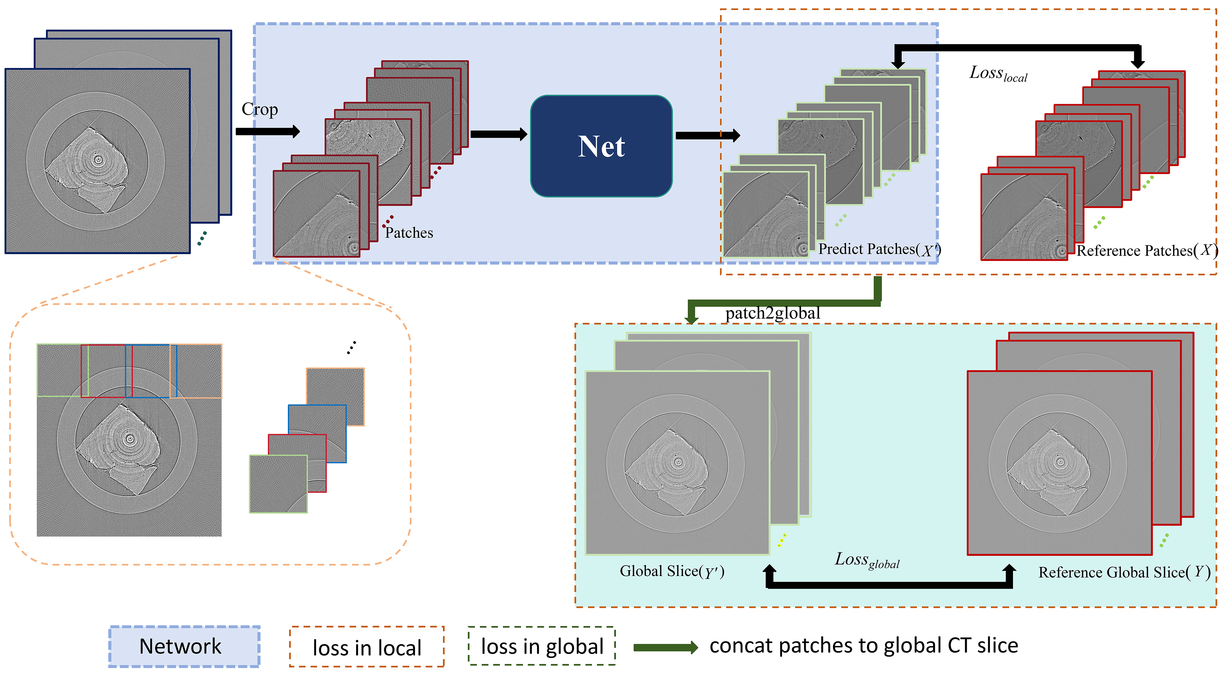
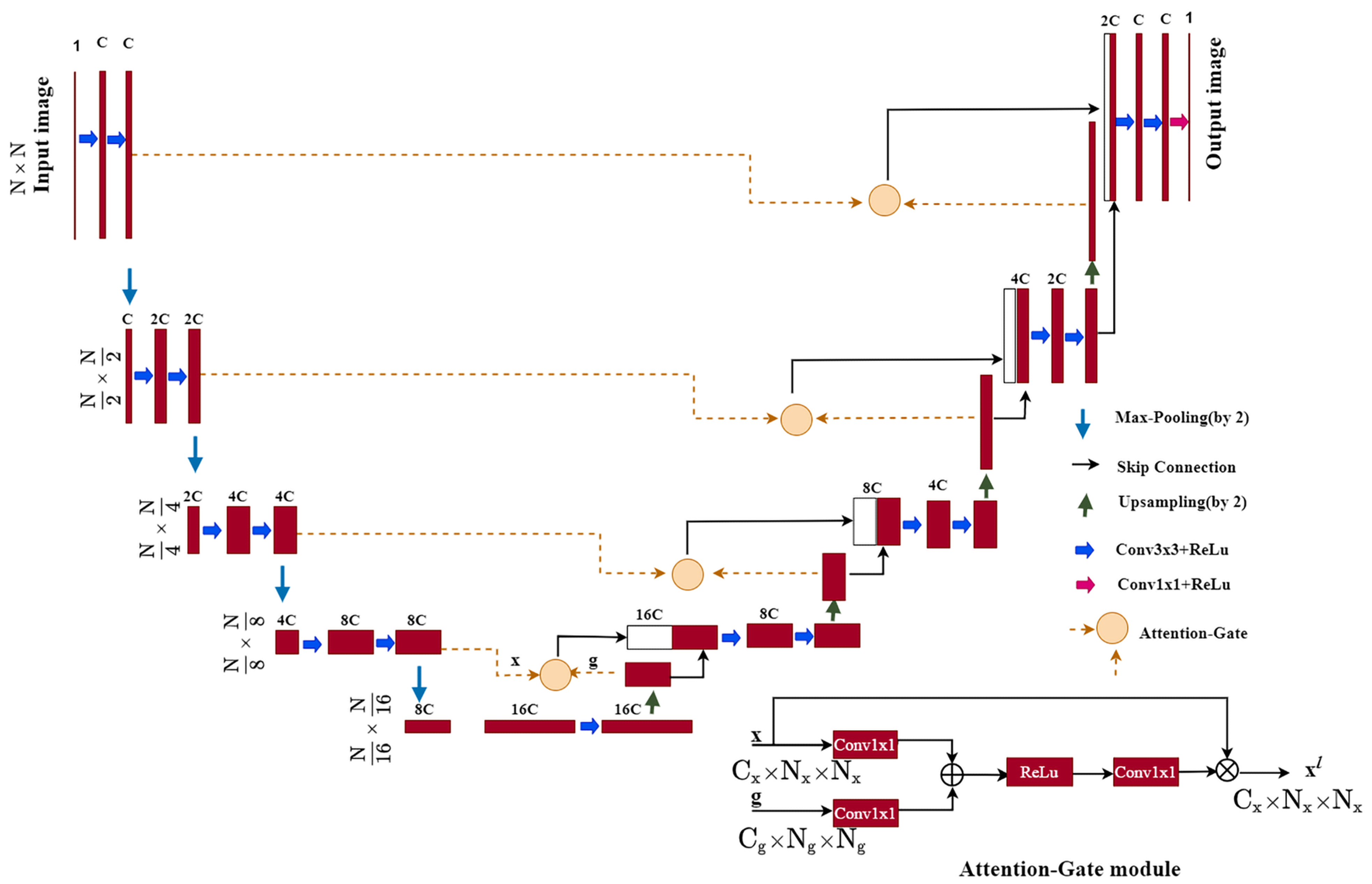
2.1. Method
2.2. Data Preparation and Image Quality Assessment
3. Results
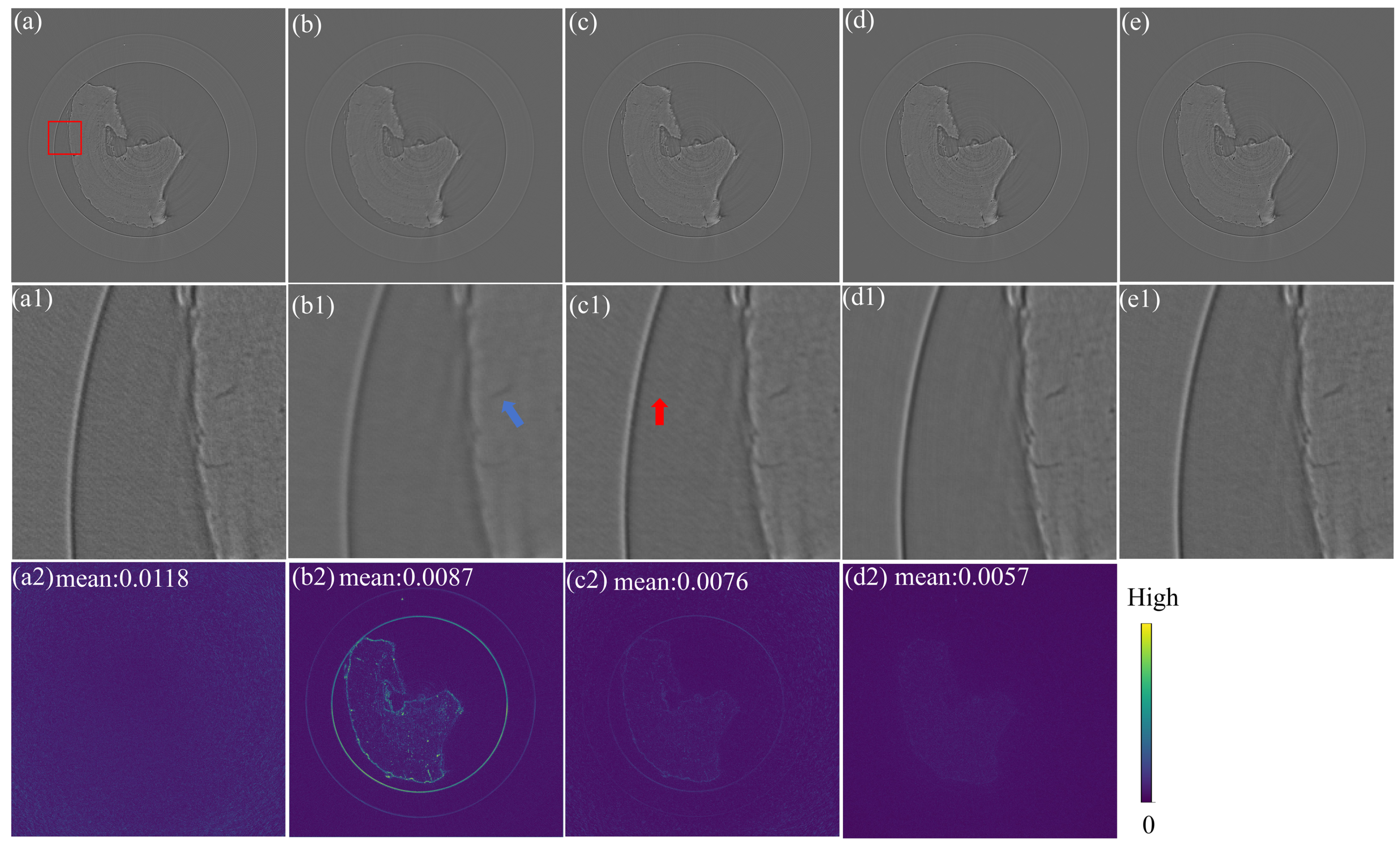
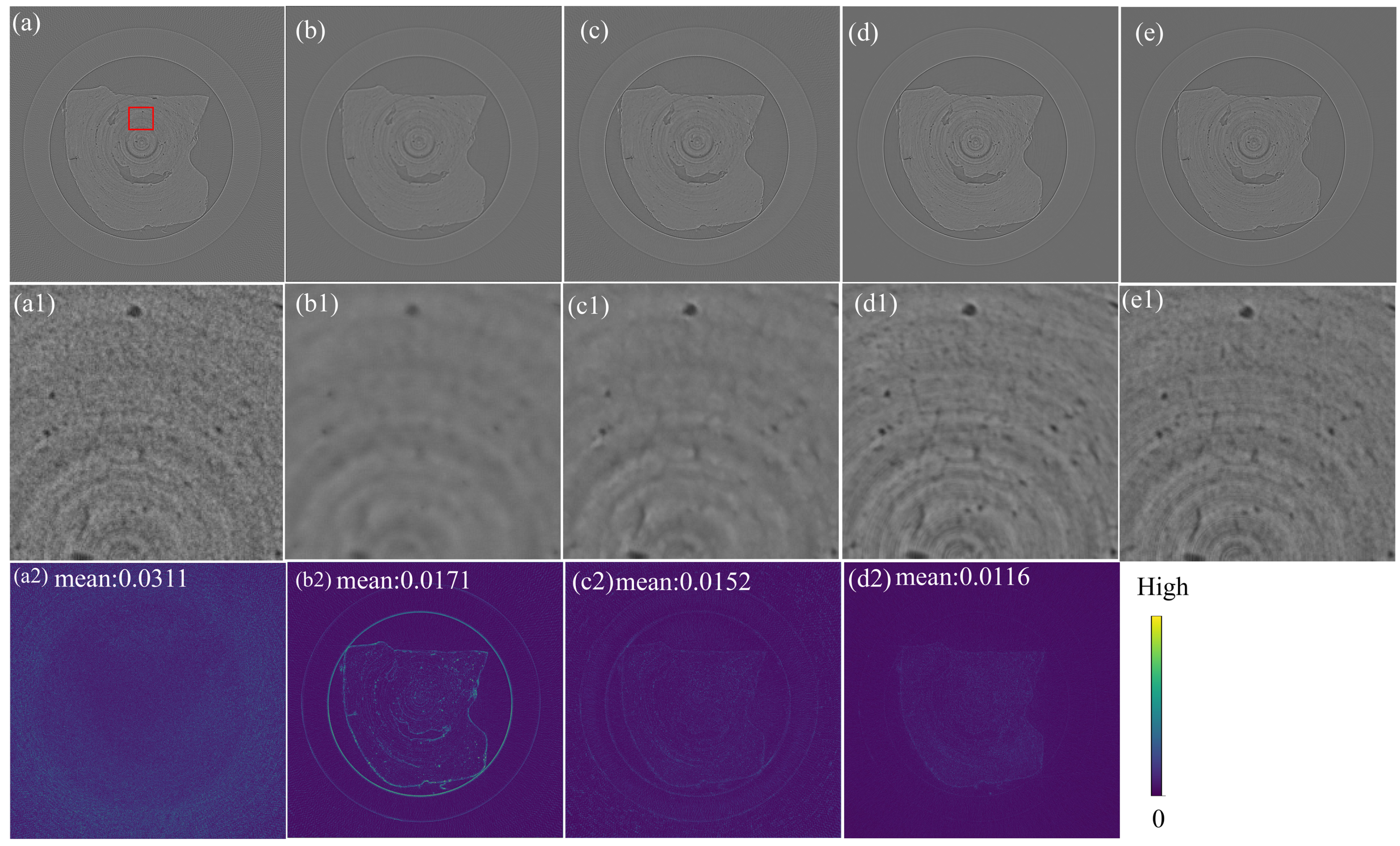
3.1. Comparison of Artifact Correction Effects of Different Methods
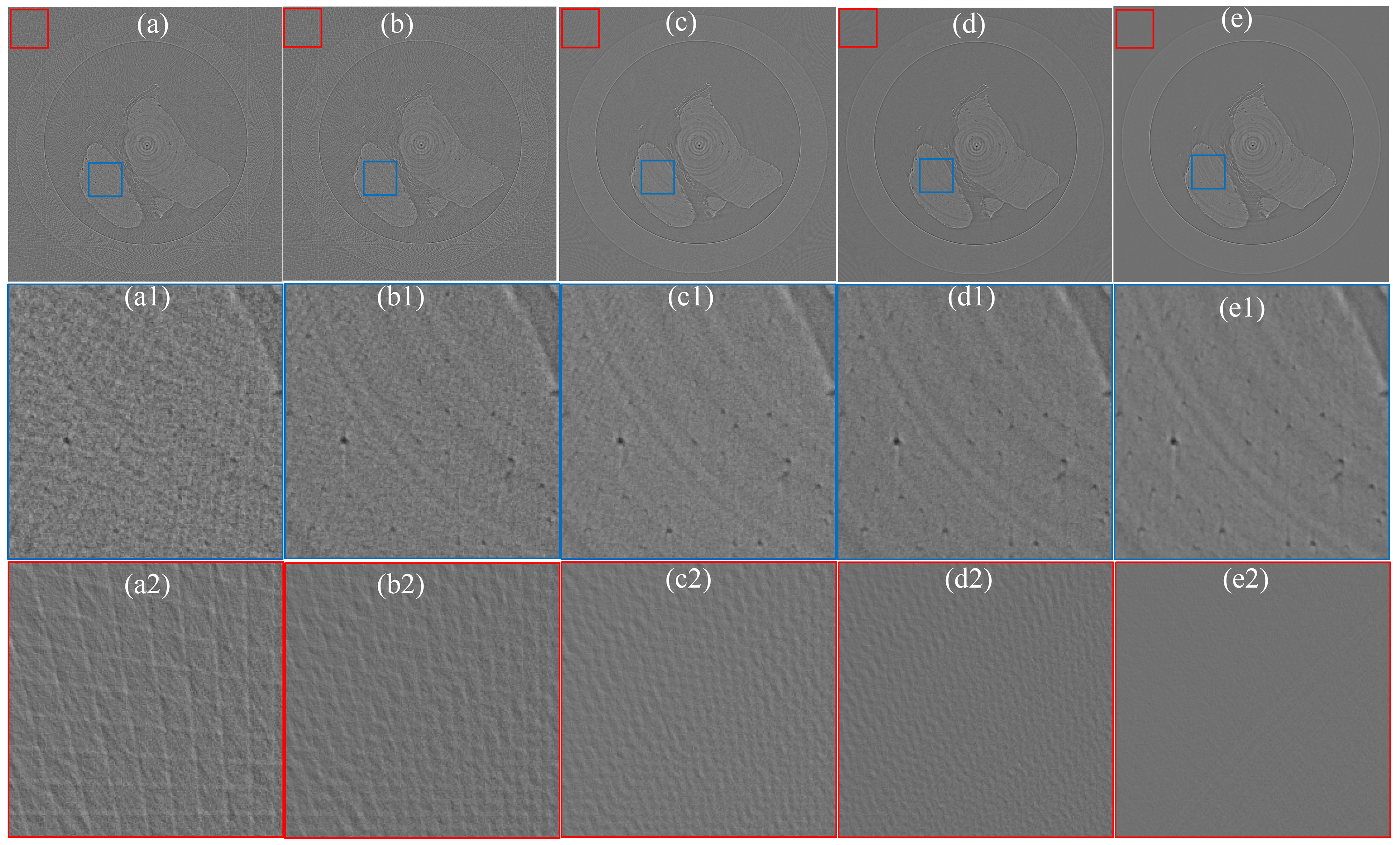
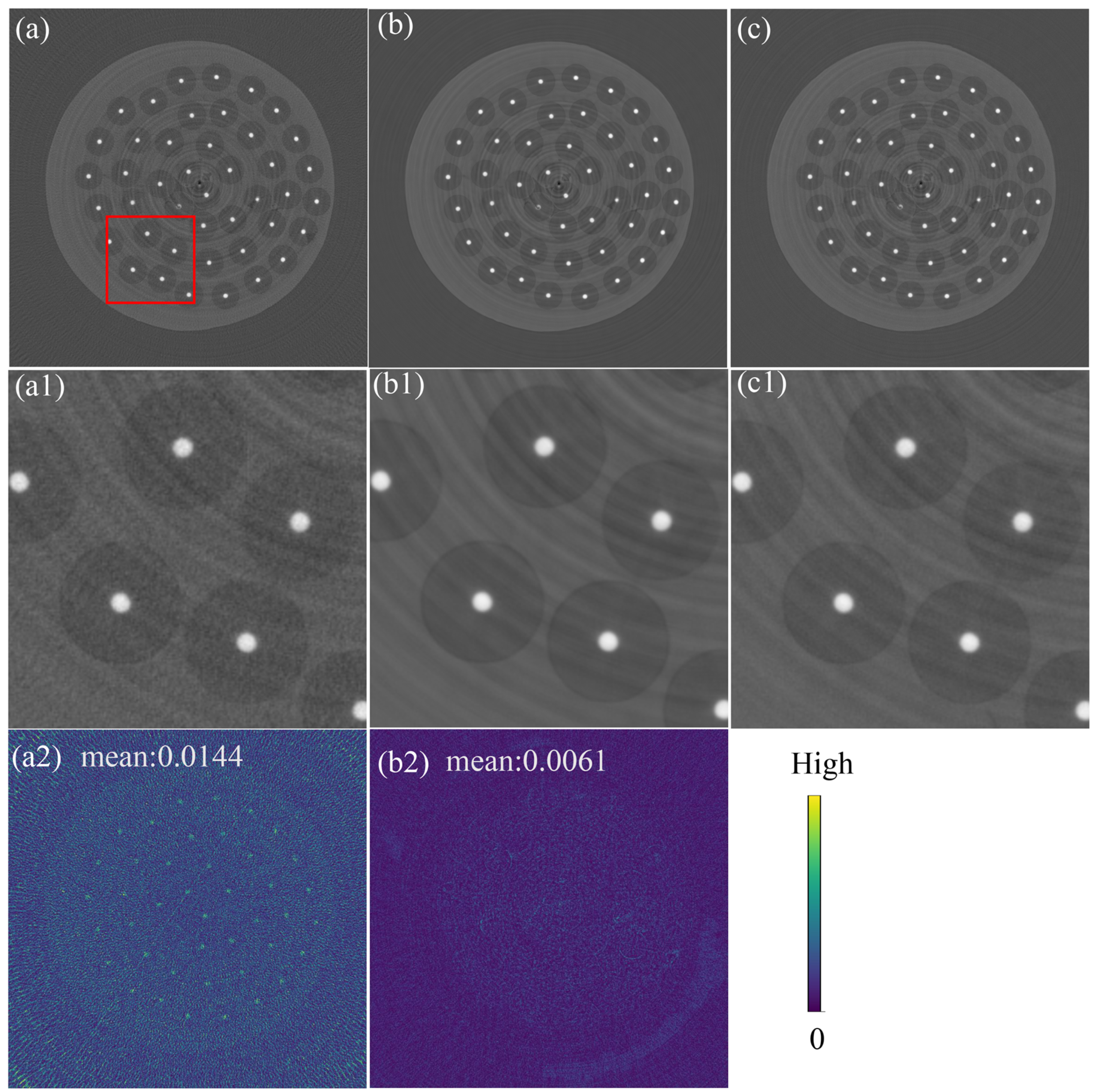
3.2. Artifact Correction Effects on Material Samples
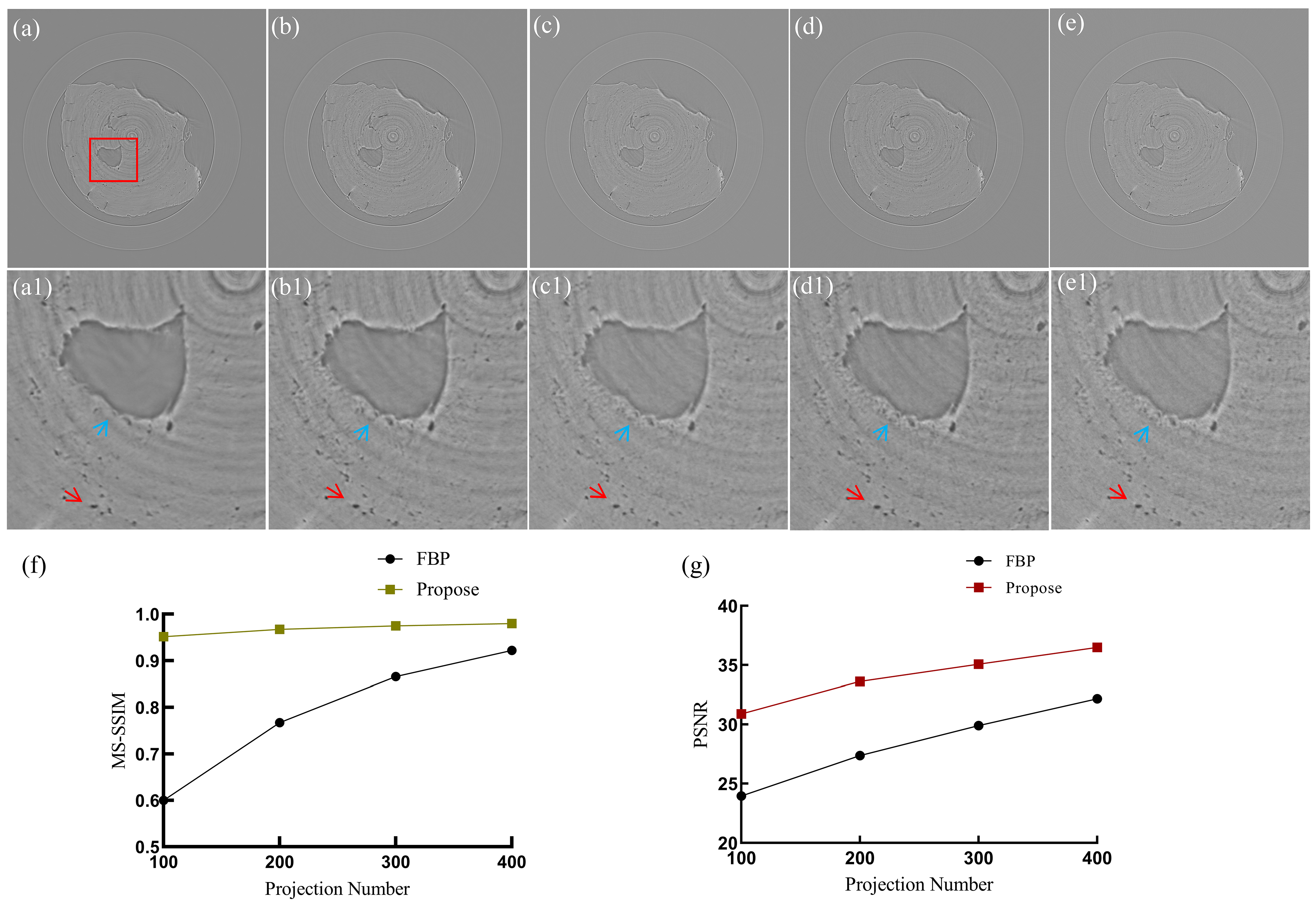
3.3. Selection of the Optimal Sparsity Ratio
4. Conclusions
Author Contributions
Funding
Institutional Review Board Statement
Informed Consent Statement
Data Availability Statement
Acknowledgments
Conflicts of Interest
Abbreviations
| CT | Computed tomography |
| FBP | Filtered back projection |
| PSNR | Peak signal-to-noise ratio |
| MS-SSIM | Multi-level structural similarity index |
References
- Kudo, H.; Suzuki, T.; Rashed, E.A. Image reconstruction for sparse-view CT and interior CT—Introduction to compressed sensing and differentiated backprojection. Quant. Imaging Med. Surg. 2013, 3, 147. [Google Scholar] [PubMed]
- Huang, J.; Ma, J.; Liu, N.; Zhang, H.; Bian, Z.; Feng, Y.; Feng, Q.; Chen, W. Sparse angular CT reconstruction using non-local means based iterative-correction POCS. Comput. Biol. Med. 2011, 41, 195–205. [Google Scholar] [CrossRef] [PubMed]
- Sidky, E.Y.; Pan, X. Image reconstruction in circular cone-beam computed tomography by constrained, total-variation minimization. Phys. Med. Biol. 2008, 53, 4777–4807. [Google Scholar] [CrossRef] [PubMed]
- Sidky, E.Y.; Kao, C.M.; Pan, X. Accurate image reconstruction from few-views and limited-angle data in divergent-beam CT. J. X-ray Sci. Technol. 2006, 14, 119–139. [Google Scholar]
- Li, H.; Chen, X.; Wang, Y.; Zhou, Z.; Zhu, Q.; Yu, D. Sparse CT reconstruction based on multi-direction anisotropic total variation (MDATV). Biomed. Eng. Online 2014, 13, 92. [Google Scholar] [CrossRef] [PubMed]
- Lou, S.; Deng, J.; Lyu, S. Chaotic signal denoising based on simplified convolutional denoising auto-encoder. Chaos Solitons Fractals 2022, 161, 112333. [Google Scholar] [CrossRef]
- Tian, C.; Fei, L.; Zheng, W.; Xu, Y.; Zuo, W.; Lin, C.W. Deep learning on image denoising: An overview. Neural Netw. 2020, 131, 251–275. [Google Scholar] [CrossRef] [PubMed]
- Du, W.; Shen, H.; Zhang, G.; Yao, X.; Fu, J. Interactive defect segmentation in X-ray images based on deep learning. Expert Syst. Appl. 2022, 198, 116692. [Google Scholar] [CrossRef]
- Al Arif, S.M.M.R.; Knapp, K.; Slabaugh, G.; Knapp, K.; Slabaugh, G. Fully automatic cervical vertebrae segmentation framework for X-ray images. Comput. Methods Programs Biomed. 2018, 157, 95–111. [Google Scholar] [CrossRef]
- Chaudhari, A.S.; Fang, Z.; Kogan, F.; Wood, J.; Stevens, K.J.; Gibbons, E.K.; Lee, J.H.; Gold, G.E.; Hargreaves, B.A. Super-resolution musculoskeletal MRI using deep learning. Magn. Reson. Med. 2018, 80, 2139–2154. [Google Scholar] [CrossRef]
- Zhong, X.; Liang, N.; Cai, A.; Yu, X.; Li, L.; Yan, B. Super-resolution image reconstruction from sparsity regularization and deep residual-learned priors. J. X-ray Sci. Technol. 2023, 31, 319–336. [Google Scholar] [CrossRef] [PubMed]
- Karamov, R.; Breite, C.; Lomov, S.V.; Sergeichev, I.; Swolfs, Y. Super-Resolution Processing of Synchrotron CT Images for Automated Fibre Break Analysis of Unidirectional Composites. Polymers 2023, 15, 2206. [Google Scholar] [CrossRef] [PubMed]
- Lee, H.; Lee, J.; Kim, H.; Cho, B.; Cho, S. Deep-neural-network-based sinogram synthesis for sparse-view CT image reconstruction. IEEE Trans. Radiat. Plasma Med. Sci. 2019, 3, 109–119. [Google Scholar] [CrossRef]
- Okamoto, T.; Ohnishi, T.; Haneishi, H. Artifact reduction for sparse-view CT using deep learning with band patch. IEEE Trans. Radiat. Plasma Med. Sci. 2022, 6, 859–873. [Google Scholar] [CrossRef]
- Jin, K.H.; McCann, M.T.; Froustey, E.; Unser, M. Deep convolutional neural network for inverse problems in imaging. IEEE Trans. Image Process. 2017, 26, 4509–4522. [Google Scholar] [CrossRef] [PubMed]
- Xie, S.; Zheng, X.; Chen, Y.; Xie, L.; Liu, J.; Zhang, Y.; Yan, J.; Zhu, H.; Hu, Y. Artifact removal using improved GoogLeNet for sparse-view CT reconstruction. Sci. Rep. 2018, 8, 6700. [Google Scholar] [CrossRef] [PubMed]
- Lee, M.; Kim, H.; Kim, H.J. Sparse-view CT reconstruction based on multi-level wavelet convolution neural network. Phys. Medica 2020, 80, 352–362. [Google Scholar] [CrossRef] [PubMed]
- Nakai, H.; Nishio, M.; Yamashita, R.; Ono, A.; Nakao, K.K.; Fujimoto, K.; Togashi, K. Quantitative and qualitative evaluation of convolutional neural networks with a deeper u-net for sparse-view computed tomography reconstruction. Acad. Radiol. 2020, 27, 563–574. [Google Scholar] [CrossRef]
- Zhang, Z.; Liang, X.; Dong, X.; Xie, Y.; Cao, G. A sparse-view CT reconstruction method based on combination of DenseNet and deconvolution. IEEE Trans. Med. Imaging 2018, 37, 1407–1417. [Google Scholar] [CrossRef]
- Han, Y.; Ye, J.C. Framing U-Net via deep convolutional framelets: Application to sparse-view CT. IEEE Trans. Med. Imaging 2018, 37, 1418–1429. [Google Scholar] [CrossRef]
- Xie, S.; Yang, T. Artifact removal in sparse-angle CT based on feature fusion residual network. IEEE Trans. Radiat. Plasma Med. Sci. 2020, 5, 261–271. [Google Scholar] [CrossRef]
- Lee, D.; Choi, S.; Kim, H.J. High quality imaging from sparsely sampled computed tomography data with deep learning and wavelet transform in various domains. Med Phys. 2019, 46, 104–115. [Google Scholar] [CrossRef] [PubMed]
- Wu, W.; Hu, D.; Niu, C.; Yu, H.; Vardhanabhuti, V.; Wang, G. DRONE: Dual-domain residual-based optimization network for sparse-view CT reconstruction. IEEE Trans. Med Imaging 2021, 40, 3002–3014. [Google Scholar] [CrossRef] [PubMed]
- Hu, D.; Liu, J.; Lv, T.; Zhao, Q.; Zhang, Y.; Quan, G.; Feng, J.; Chen, Y.; Luo, L. Hybrid-domain neural network processing for sparse-view CT reconstruction. IEEE Trans. Radiat. Plasma Med Sci. 2020, 5, 88–98. [Google Scholar] [CrossRef]
- Li, R.; Li, Q.; Wang, H.; Li, S.; Zhao, J.; Yan, Q.; Wang, L. DDPTransformer: Dual-Domain With Parallel Transformer Network for Sparse View CT Image Reconstruction. IEEE Trans. Comput. Imaging 2022, 8, 1101–1116. [Google Scholar] [CrossRef]
- Cheslerean-Boghiu, T.; Hofmann, F.C.; Schultheiß, M.; Pfeiffer, F.; Pfeiffer, D.; Lasser, T. Wnet: A data-driven dual-domain denoising model for sparse-view computed tomography with a trainable reconstruction layer. IEEE Trans. Comput. Imaging 2023, 9, 120–132. [Google Scholar] [CrossRef]
- Dong, X.; Vekhande, S.; Cao, G. Sinogram interpolation for sparse-view micro-CT with deep learning neural network. In Proceedings of the Medical Imaging 2019: Physics of Medical Imaging; SPIE: Toronto, ON, Canada, 2019; Volume 10948, pp. 692–698. [Google Scholar]
- Ronneberger, O.; Fischer, P.; Brox, T. U-net: Convolutional networks for biomedical image segmentation. In Proceedings of the Medical Image Computing and Computer-Assisted Intervention–MICCAI 2015: 18th International Conference, Munich, Germany, 5–9 October 2015; Proceedings, Part III 18. Springer: Berlin, Germany, 2015; pp. 234–241. [Google Scholar]
- Yagi, N.; Inoue, K.; Oka, T. CCD-based X-ray area detector for time-resolved diffraction experiments. J. Synchrotron Radiat. 2004, 11, 456–461. [Google Scholar] [CrossRef] [PubMed]
- Stampanoni, M.; Groso, A.; Isenegger, A.; Mikuljan, G.; Chen, Q.; Bertrand, A.; Henein, S.; Betemps, R.; Frommherz, U.; Böhler, P.; et al. Trends in synchrotron-based tomographic imaging: The SLS experience. In Proceedings of the Developments in X-ray Tomography V; SPIE: Toronto, ON, Canada, 2006; Volume 6318, pp. 193–206. [Google Scholar]
- Oktay, O.; Schlemper, J.; Folgoc, L.L.; Lee, M.; Heinrich, M.; Misawa, K.; Mori, K.; McDonagh, S.; Hammerla, N.Y.; Kainz, B.; et al. Attention u-net: Learning where to look for the pancreas. arXiv 2018, arXiv:1804.03999. [Google Scholar]
- Wang, Z.; Bovik, A.C.; Sheikh, H.R.; Simoncelli, E.P. Image quality assessment: From error visibility to structural similarity. IEEE Trans. Image Process. 2004, 13, 600–612. [Google Scholar] [CrossRef]
- Rukundo, O. Normalized Weighting Schemes for Image Interpolation Algorithms. Appl. Sci. 2023, 13, 1741. [Google Scholar] [CrossRef]
- Wang, Z.; Simoncelli, E.P.; Bovik, A.C. Multiscale structural similarity for image quality assessment. In Proceedings of the Thrity-Seventh Asilomar Conference on Signals, Systems & Computers, Pacific Grove, CA, USA, 9–12 November 2003; IEEE: Piscataway, NJ, USA, 2003; Volume 2, pp. 1398–1402. [Google Scholar]


| Methods | 200 Views (PSNR) | 200 Views (MS-SSIM) |
|---|---|---|
| FBP | 27.3812 | 0.7672 |
| DD-Net | 28.5358 | 0.9261 |
| FBPConvNet | 32.3808 | 0.9263 |
| Proposed method | 33.6259 | 0.9673 |
| Methods | 400 Views (PSNR) | 400 Views (MS-SSIM) |
|---|---|---|
| FBP | 32.1820 | 0.9218 |
| DD-Net | 33.7385 | 0.9589 |
| FBPConvNet | 35.4875 | 0.9671 |
| Proposed method | 36.4845 | 0.9800 |
Disclaimer/Publisher’s Note: The statements, opinions and data contained in all publications are solely those of the individual author(s) and contributor(s) and not of MDPI and/or the editor(s). MDPI and/or the editor(s) disclaim responsibility for any injury to people or property resulting from any ideas, methods, instructions or products referred to in the content. |
© 2024 by the authors. Licensee MDPI, Basel, Switzerland. This article is an open access article distributed under the terms and conditions of the Creative Commons Attribution (CC BY) license (https://creativecommons.org/licenses/by/4.0/).
Share and Cite
Huang, M.; Li, G.; Sun, R.; Zhang, J.; Wang, Z.; Wang, Y.; Deng, T.; Yu, B. Sparse-View Artifact Correction of High-Pixel-Number Synchrotron Radiation CT. Appl. Sci. 2024, 14, 3397. https://doi.org/10.3390/app14083397
Huang M, Li G, Sun R, Zhang J, Wang Z, Wang Y, Deng T, Yu B. Sparse-View Artifact Correction of High-Pixel-Number Synchrotron Radiation CT. Applied Sciences. 2024; 14(8):3397. https://doi.org/10.3390/app14083397
Chicago/Turabian StyleHuang, Mei, Gang Li, Rui Sun, Jie Zhang, Zhimao Wang, Yanping Wang, Tijian Deng, and Bei Yu. 2024. "Sparse-View Artifact Correction of High-Pixel-Number Synchrotron Radiation CT" Applied Sciences 14, no. 8: 3397. https://doi.org/10.3390/app14083397
APA StyleHuang, M., Li, G., Sun, R., Zhang, J., Wang, Z., Wang, Y., Deng, T., & Yu, B. (2024). Sparse-View Artifact Correction of High-Pixel-Number Synchrotron Radiation CT. Applied Sciences, 14(8), 3397. https://doi.org/10.3390/app14083397