
Study on the Oil Spill Transport Behavior and Multifactorial Effects of the Lancang River Crossing Pipeline

Abstract
:1. Introduction
2. Materials and Methods
2.1. Hydrodynamic Model
2.2. Oil Spill Model
2.2.1. Diffusion and Drift of Oil Film
2.2.2. Weathering of Oil Spill
2.3. Model Construction
2.3.1. Hydrodynamic Model Construction
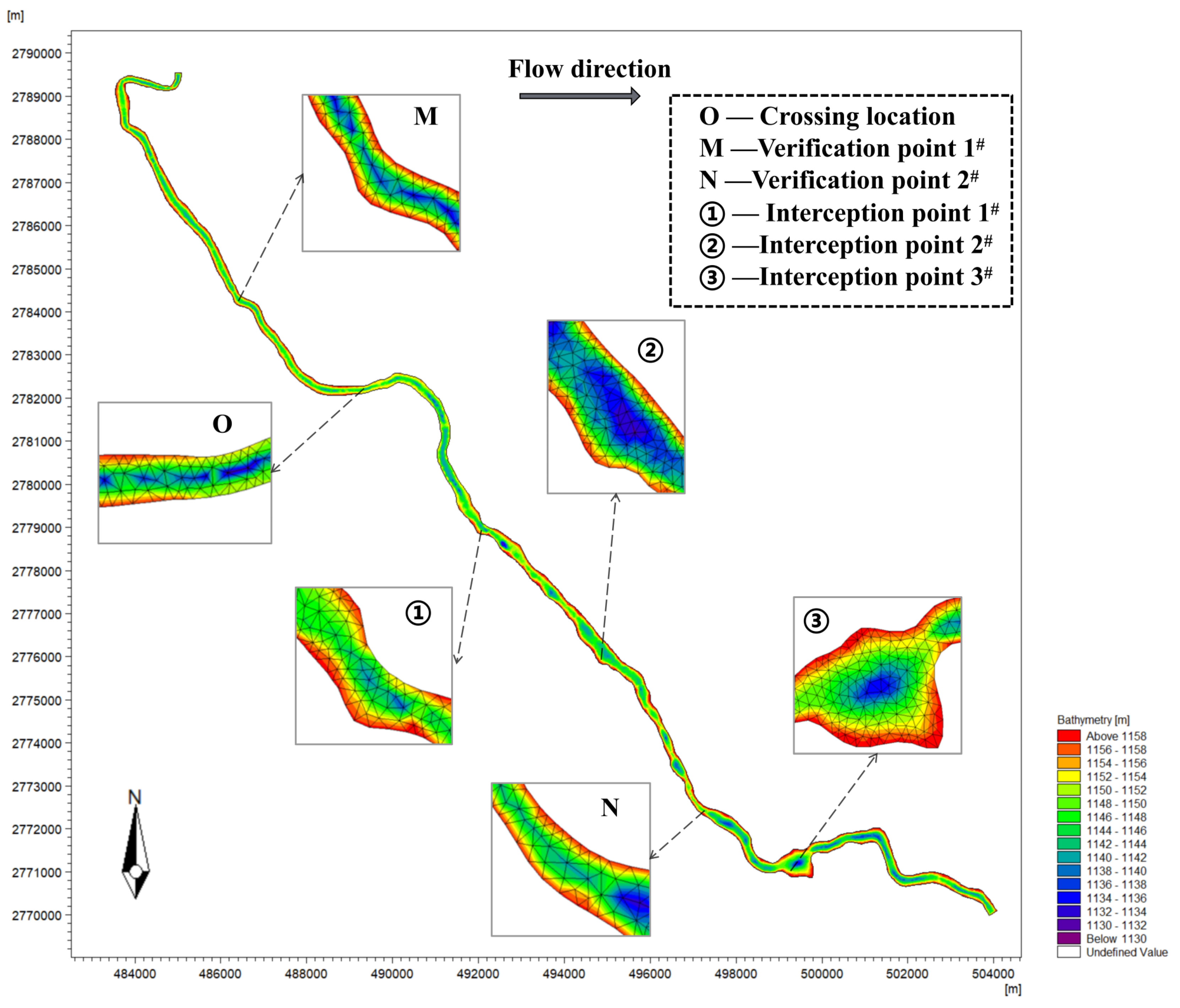
2.3.2. Model Validation
3. Results and Discussions
3.1. Simulation
3.1.1. Simulation Scenario Setting
- River flow. As a typical monsoon river, the Lancang River has a large variation of flow under different water periods. According to the hydrological data of the basin, the value of the river flow in this study is selected between the minimum flow in the dry season and the maximum flow in the abundant season, ranging from 500 m3/s to 7000 m3/s;
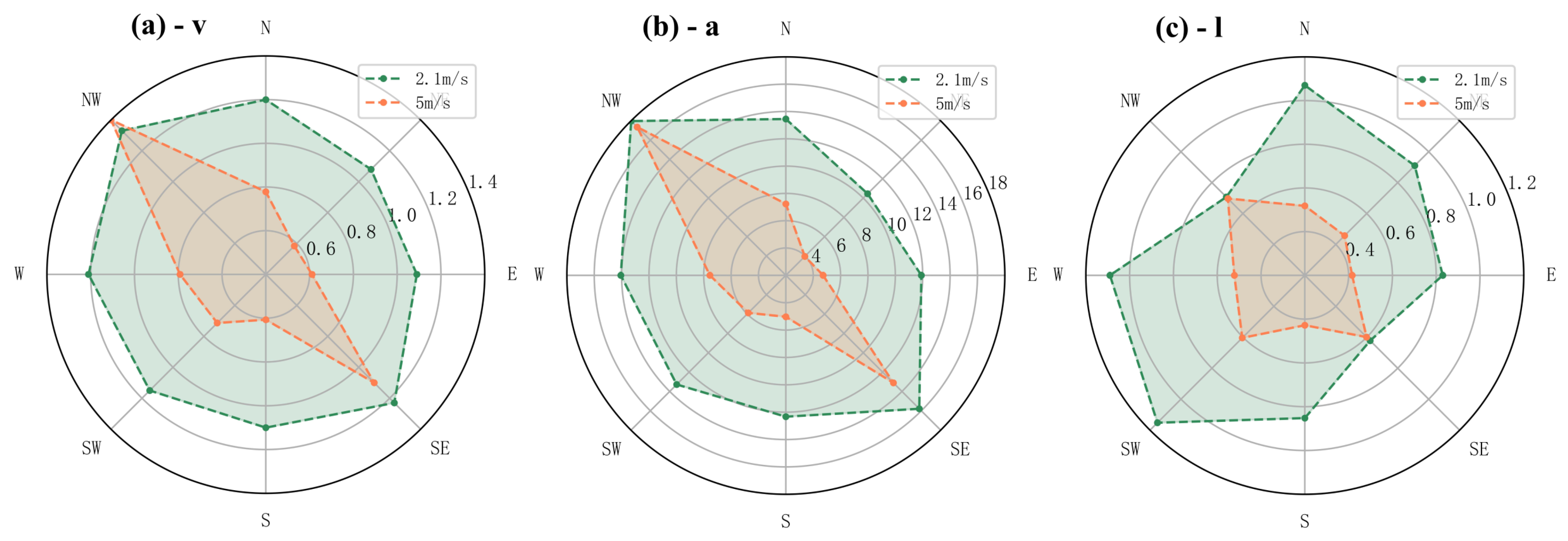
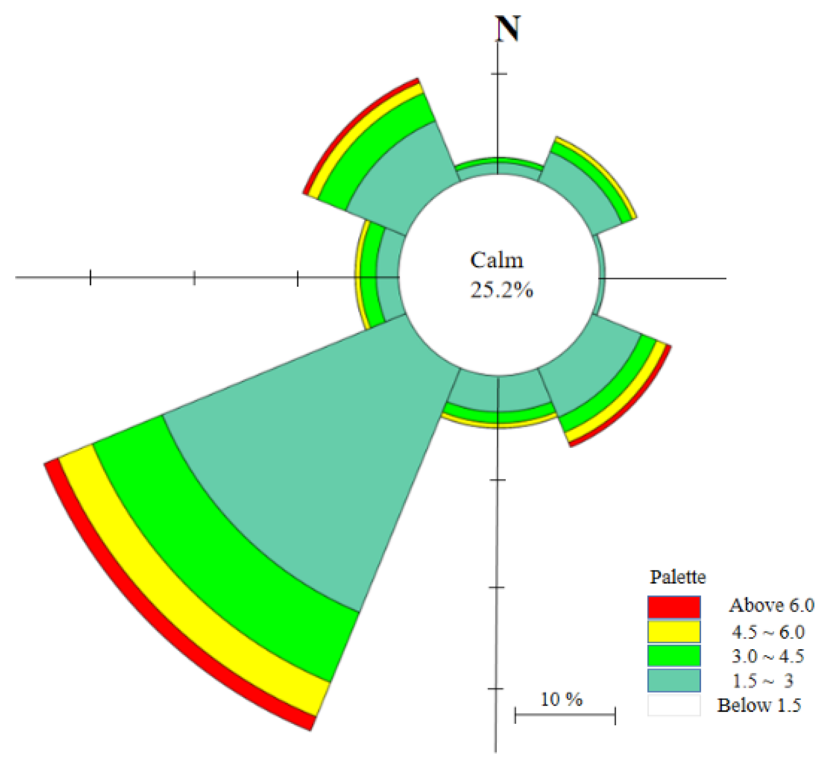
- Wind, including wind speed and direction. Based on the wind data provided for 2021 and 2022, a rose wind map was produced, as shown in Figure 4. The average annual wind speed in the region is 2.1 m/s, and the main wind direction is southwest. The variables of wind speed were set from 1 m/s to 7 m/s, and the variables of wind direction were set in 8 directions;
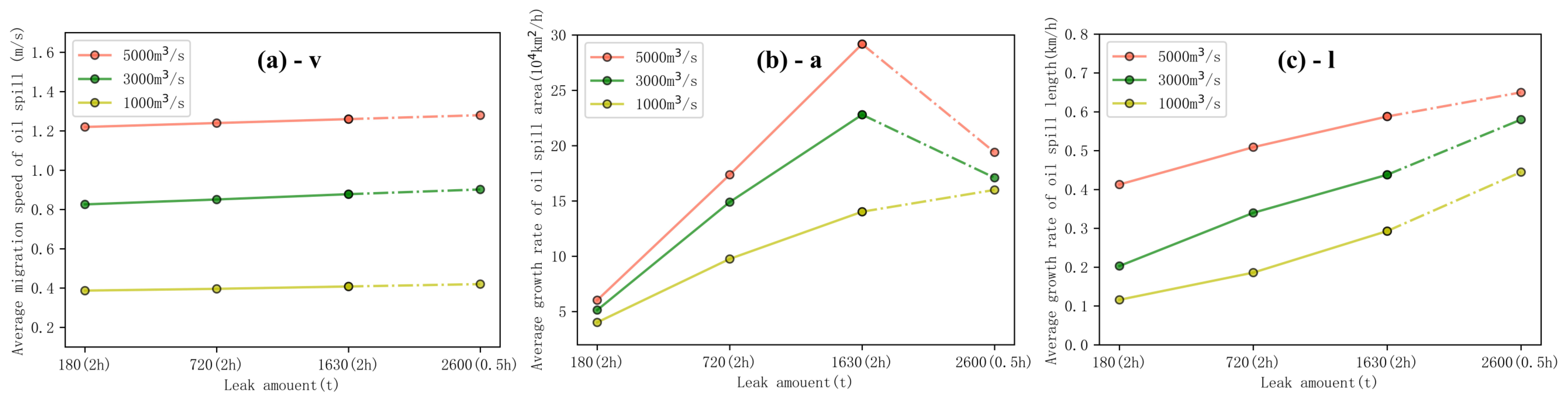
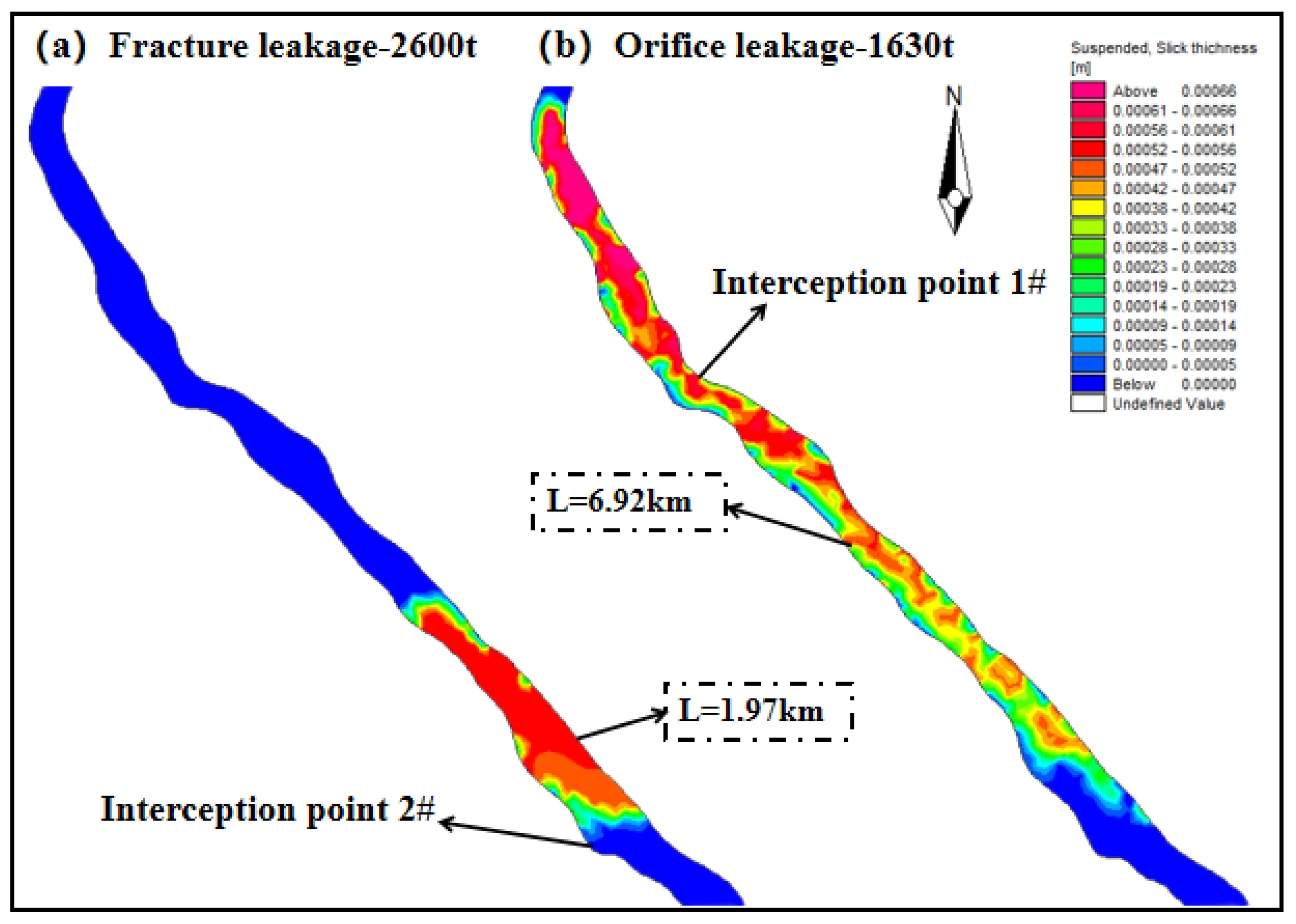
- Leakage modes. Leakage modes include fracture leakage and perforation leakage. According to the researched literature [42], when the pipeline section is fractured, from the beginning of the accident to the upstream and downstream valve closure, all the crude oil in the pipeline will be leaked into the Lancang River within 0.5 h; when the pipeline is perforated and leaked, the maintenance personnel can complete the emergency blocking operation within 2 h. The amount of leakage under the fracture leakage mode was calculated to be 2600 t; under the perforation leakage mode, the leakage hole size was set to be 5%D, 10%D, and 15%D (D is the outer diameter of the pipe of 813 mm), and the amount of leakage was 180 t, 720 t, and 1630 t, respectively.
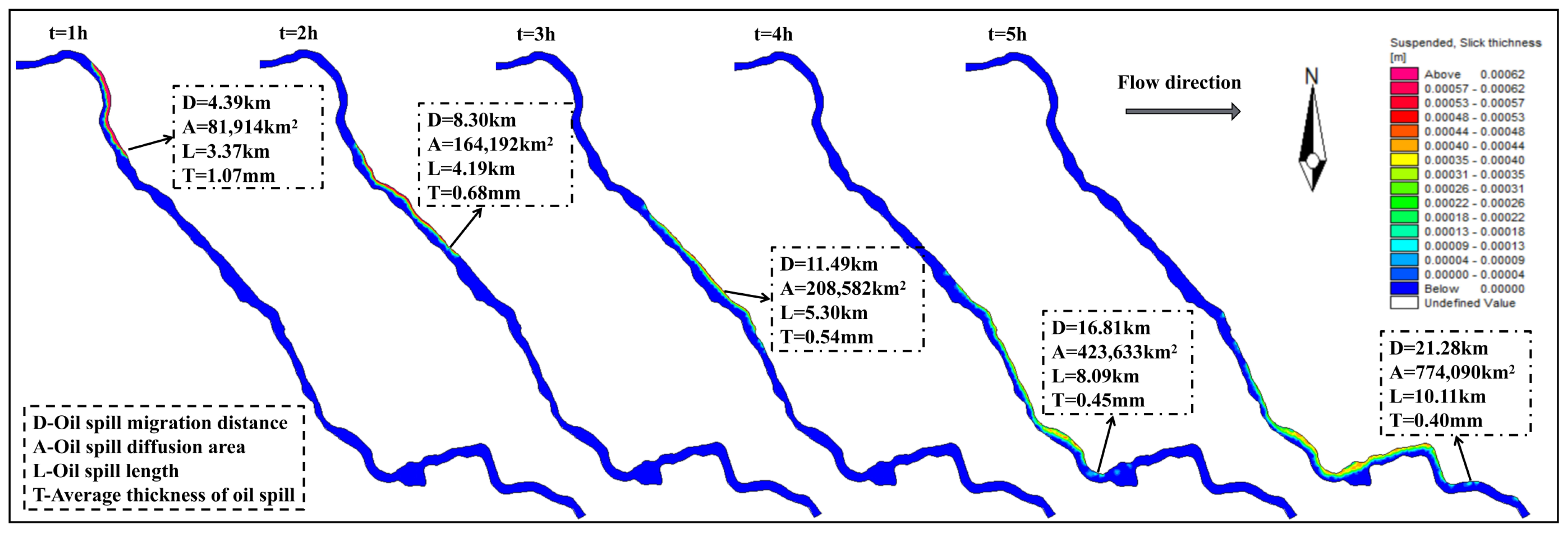
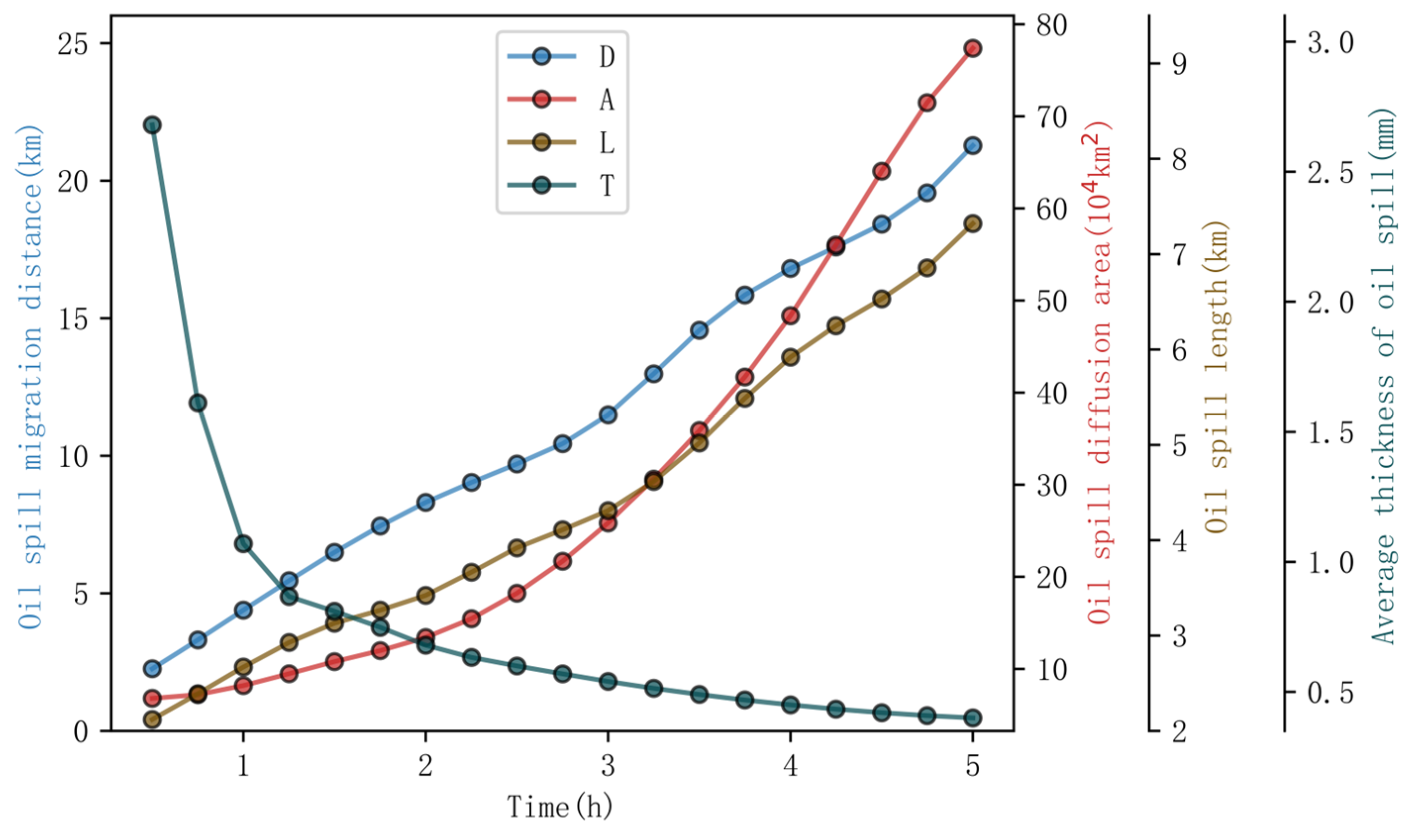
3.1.2. Simulation Results
3.2. Oil Spill Transport Behavior under Various Influencing Factors
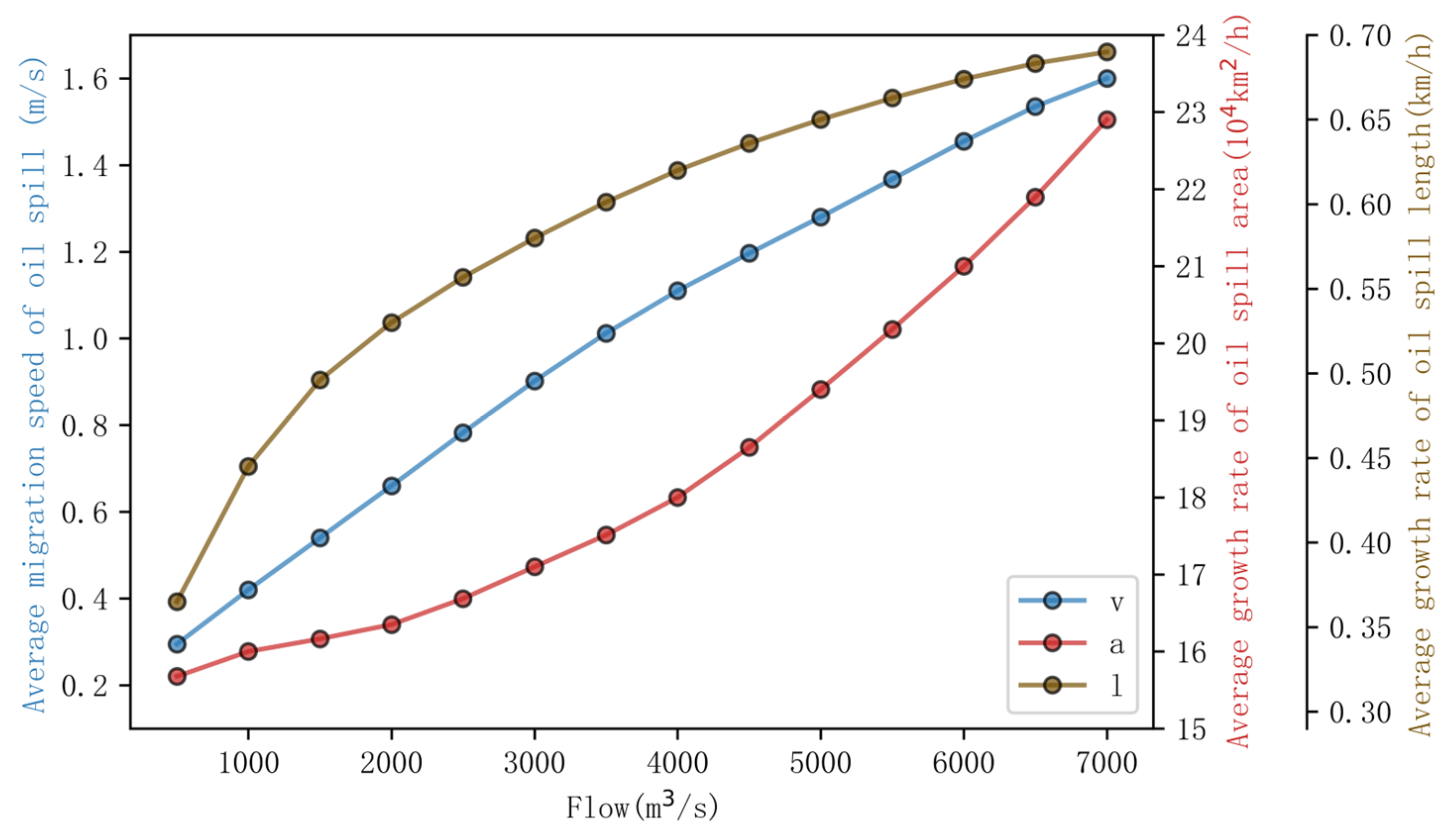
3.2.1. River Flow
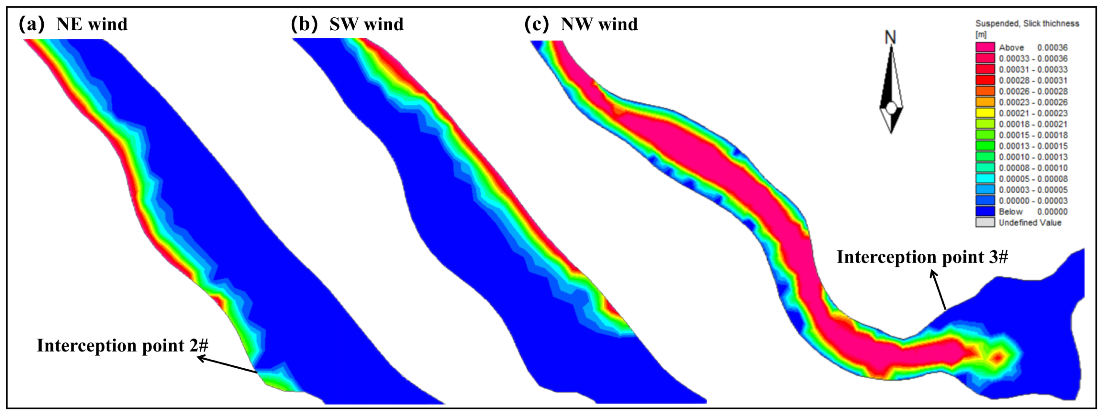
3.2.2. Wind
3.2.3. Leakage Mode
3.3. Prediction of Oil Spill Transport Behavior Based on Machine Learning
4. Conclusions
- (1)
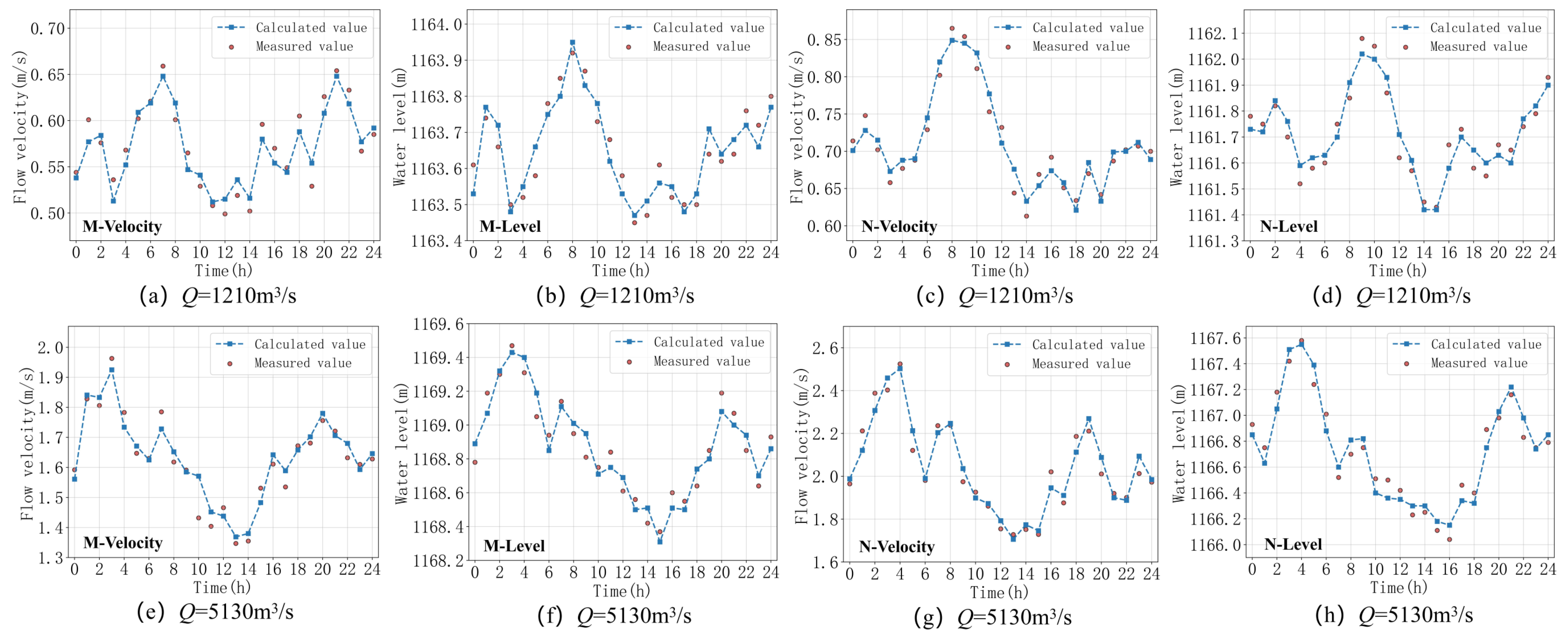
- For the two-dimensional hydrodynamic model of the Lancang River crude oil crossing pipeline basin, the flow velocity and water level of the model were verified according to the measured hydrological data. The MAE of the flow velocity is 0.054 m/s, and the MAE of the water level is 0.062 m. The simulated values are in good agreement with the actual values. It shows that the model is suitable for the study of oil spill transport behavior in this basin.
- (2)
- The transport behavior of oil spills under different spill scenarios was simulated. It was found that the higher the river flow, the faster the migration, diffusion, and longitudinal extension behavior of the oil spill; under downwind and headwind conditions, the effects of wind speed on the oil spill transport behavior are small. In the remaining wind directions, the migration and diffusion behaviors of the oil spill will slow down with the increase of wind speed, and the longitudinal extension behaviors of the oil spill will speed up firstly and then slow down with the increase of wind speed; the effects of leakage mode on the migration rate of the oil spill are small. Under the perforation leakage, the increase in oil spill volume will make the oil spill diffuse and extend longitudinally in the river channel faster. The simulation results can provide guidance for the development of emergency response plans for river crossing pipeline oil spill accidents.
- (3)
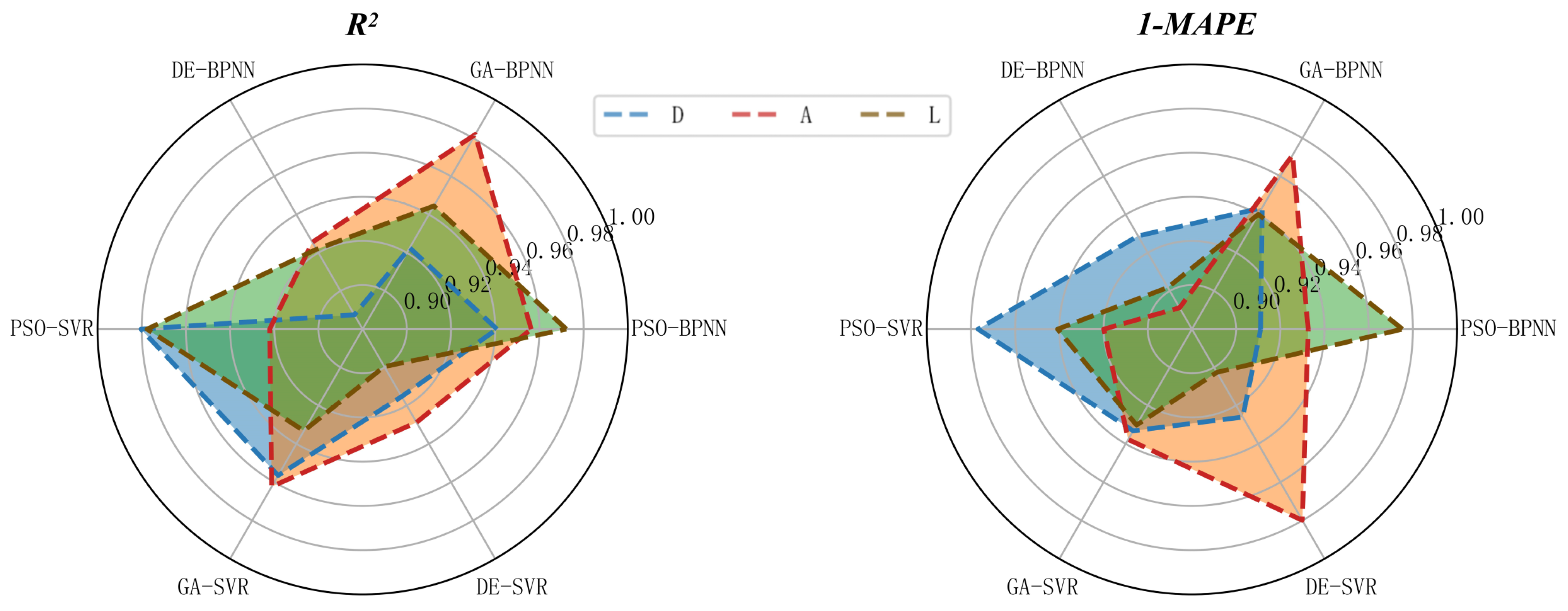
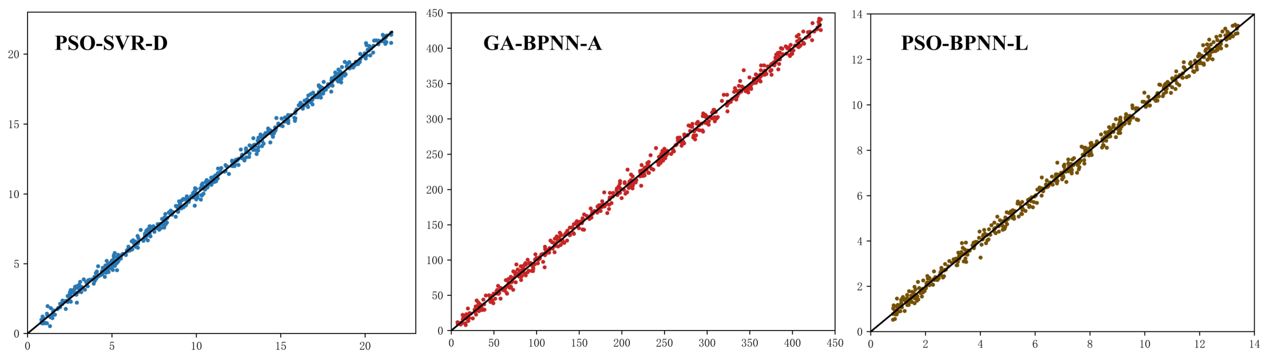
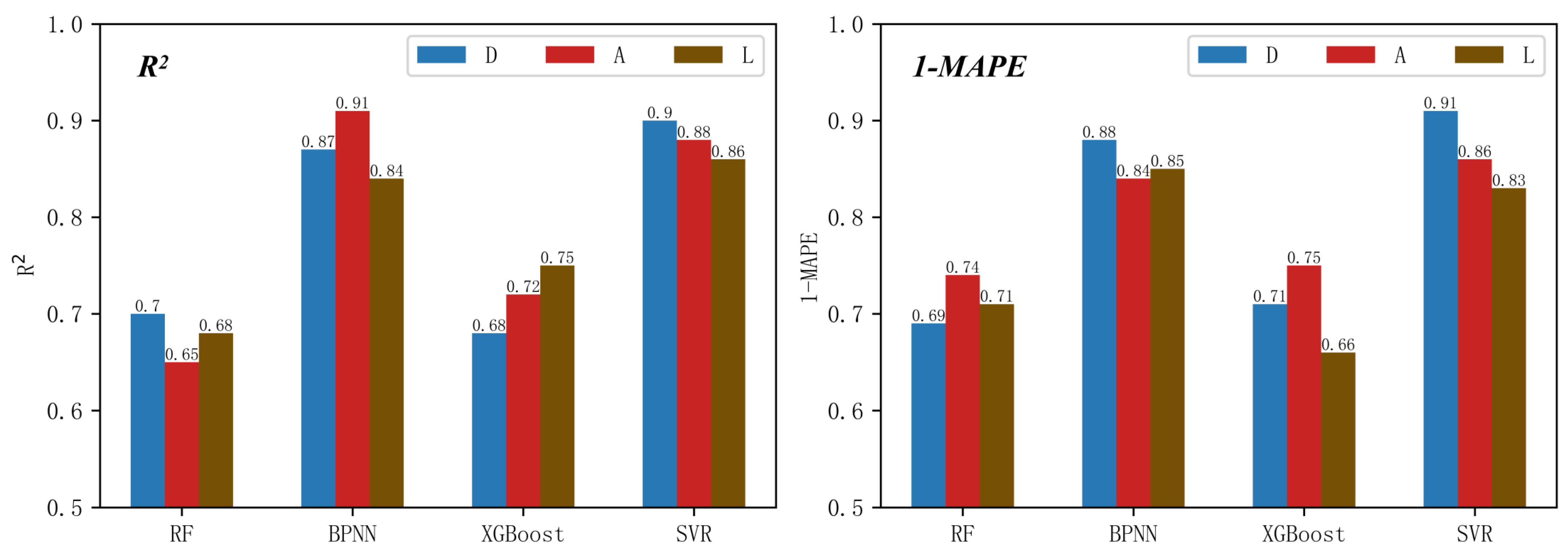
- An oil spill transport state dataset was established through 320 sets of numerical experiments. The oil spill transport state prediction model was established by machine learning combination algorithms. The three machine learning algorithms, PSO-SVR, GA-BPNN, and PSO-BPNN, have the best performance in predicting the oil spill migration distance, oil spill area, and oil spill contaminated zone length, respectively, with the R2 and 1-MAPE above 0.971, and the accuracy of the prediction model is high. The model can provide support for rapid emergency response to sudden oil spill accidents of river crossing pipelines.
Author Contributions
Funding
Institutional Review Board Statement
Informed Consent Statement
Data Availability Statement
Conflicts of Interest
References
- Chen, J.; Zhang, W.; Wan, Z.; Li, S.; Huang, T.; Fei, Y. Oil spills from global tankers: Status review and future governance. J. Clean. Prod. 2019, 227, 20–32. [Google Scholar] [CrossRef]
- Kvočka, D.; Žagar, D.; Banovec, P. A Review of River Oil Spill Modeling. Water 2021, 13, 1620. [Google Scholar] [CrossRef]
- Kabyl, A.; Yang, M.; Shah, D.; Ahmad, A. Bibliometric Analysis of Accidental Oil Spills in Ice-Infested Waters. Int. J. Environ. Res. Public Health 2022, 19, 15190. [Google Scholar] [CrossRef] [PubMed]
- Yang, Y.-F.; Wang, S.; Zhu, Z.-D.; Jin, L.-Z. Prediction model and consequence analysis for riverine oil spills. Front. Environ. Sci. 2022, 10, 1054839. [Google Scholar] [CrossRef]
- Liu, Z.; Chen, Q.; Zhang, Y.; Zheng, C.; Cai, B.; Liu, Y. Research on transport and weathering of oil spills in Jiaozhou Bight, China. Reg. Stud. Mar. Sci. 2022, 51, 102197. [Google Scholar] [CrossRef]
- Lewis, D.; Sauzier, J. Cleaning up after Mauritius oil spill. Nature 2020, 585, 172. [Google Scholar] [CrossRef] [PubMed]
- Chen, J.; Di, Z.; Shi, J.; Shu, Y.; Wan, Z.; Song, L.; Zhang, W. Marine oil spill pollution causes and governance: A case study of Sanchi tanker collision and explosion. J. Clean. Prod. 2020, 273, 122978. [Google Scholar] [CrossRef]
- Aljaroudi, A.; Khan, F.; Akinturk, A.; Haddara, M.; Thodi, P. Risk assessment of offshore crude oil pipeline failure. J. Loss Prev. Process Ind. 2015, 37, 101–109. [Google Scholar] [CrossRef]
- Aa, I.; Op, A.; Ujj, I.; Mt, B. A critical review of oil spills in the Niger Delta aquatic environment: Causes, impacts, and bioremediation assessment. Environ. Monit. Assess. 2022, 194, 816. [Google Scholar] [CrossRef] [PubMed]
- Ganju, N.K.; Brush, M.J.; Rashleigh, B.; Aretxabaleta, A.L.; del Barrio, P.; Grear, J.S.; Harris, L.A.; Lake, S.J.; McCardell, G.; O’donnell, J.; et al. Progress and Challenges in Coupled Hydrodynamic-Ecological Estuarine Modeling. Estuaries Coasts 2016, 39, 311–332. [Google Scholar] [CrossRef]
- Shen, Y.X.; Jiang, C.B. A comprehensive review of watershed flood simulation model. Nat. Hazards 2023, 118, 875–902. [Google Scholar] [CrossRef]
- Munar, A.M.; Cavalcanti, J.R.; Bravo, J.M.; Fan, F.M.; da Motta-Marques, D.; Fragoso, C.R., Jr. Coupling large-scale hydrological and hydrodynamic modeling: Toward a better comprehension of watershed-shallow lake processes. J. Hydrol. 2018, 564, 424–441. [Google Scholar] [CrossRef]
- De Goede, E.D. Historical overview of 2D and 3D hydrodynamic modelling of shallow water flows in the Netherlands. Ocean Dyn. 2020, 70, 521–539. [Google Scholar] [CrossRef]
- Keramea, P.; Kokkos, N.; Zodiatis, G.; Sylaios, G. Modes of Operation and Forcing in Oil Spill Modeling: State-of-Art, Deficiencies and Challenges. J. Mar. Sci. Eng. 2023, 11, 1165. [Google Scholar] [CrossRef]
- Spaulding, M.L. State of the art review and future directions in oil spill modeling. Mar. Pollut. Bull. 2017, 115, 7–19. [Google Scholar] [CrossRef] [PubMed]
- Hou, X.; Hodges, B.R.; Feng, D.; Liu, Q. Uncertainty quantification and reliability assessment in operational oil spill forecast modeling system. Mar. Pollut. Bull. 2017, 116, 420–433. [Google Scholar] [CrossRef] [PubMed]
- Azevedo, A.; Oliveira, A.; Fortunato, A.B.; Zhang, J.; Baptista, A.M. A cross-scale numerical modeling system for management support of oil spill accidents. Mar. Pollut. Bull. 2014, 80, 132–147. [Google Scholar] [CrossRef] [PubMed]
- Kuang, C.; Chen, J.; Wang, J.; Qin, R.; Fan, J.; Zou, Q. Effect of Wind-Wave-Current Interaction on Oil Spill in the Yangtze River Estuary. J. Mar. Sci. Eng. 2023, 11, 494. [Google Scholar] [CrossRef]
- Liu, D.; Mu, L.; Ha, S.; Wang, S.; Zhao, E. An innovative coupling technique for integrating oil spill prediction model with finite volume method-based ocean model. Mar. Pollut. Bull. 2022, 185, 114242. [Google Scholar] [CrossRef]
- Zhen, Z.; Li, D.; Li, Y.; Chen, S.; Bu, S. Trajectory and weathering of oil spill in Daya bay, the South China sea. Environ. Pollut. 2020, 267, 115562. [Google Scholar] [CrossRef]
- Periáñez, R. A Lagrangian oil spill transport model for the Red Sea. Ocean Eng. 2020, 217, 107953. [Google Scholar] [CrossRef]
- Bozkurtoglu, S.N.E. Modeling oil spill trajectory in Bosphorus for contingency planning. Mar. Pollut. Bull. 2017, 123, 57–72. [Google Scholar] [CrossRef] [PubMed]
- Da Cunha, A.C.; De Abreu, C.H.M.; Crizanto, J.L.P.; Cunha, H.F.A.; Brito, A.U.; Pereira, N.N. Modeling pollutant dispersion scenarios in high vessel-traffic areas of the Lower Amazon River. Mar. Pollut. Bull. 2021, 168, 112404. [Google Scholar] [CrossRef]
- Jiang, P.; Tong, S.; Wang, Y.; Xu, G. Modelling the oil spill transport in inland waterways based on experimental study. Environ. Pollut. 2021, 284, 117473. [Google Scholar] [CrossRef]
- Wang, J.; Wang, S.; Zhu, Z.; Yang, Y.; Zhang, Q.; Xu, S.; Yan, J. Integrated framework for assessing the impact of inland oil spills on a river basin: Model and case study in China. Ecol. Indic. 2024, 158, 111576. [Google Scholar] [CrossRef]
- Mendoza-Cantú, A.; Heydrich, S.C.; Cervantes, I.S.; Orozco, O.O. Identification of environmentally vulnerable areas with priority for prevention and management of pipeline crude oil spills. J. Environ. Manag. 2011, 92, 1706–1713. [Google Scholar] [CrossRef] [PubMed]
- García, H.; Nieves, C.; Colonia, J.D. Integrity management program for geo-hazards in the ocensa pipeline system. In Proceedings of the ASME International Pipeline Conference, Calgary, AB, Canada, 27 September–1 October 2010; Volume 4, p. 415. [Google Scholar]
- Zhao, X.B.; Xu, B.; Huang, X.L. The Situation and Countermeasures of Oil Spill Control of Inland River Ships, 018(001); China Water Transp.: Wuhan, China, 2018; pp. 146–148. [Google Scholar]
- Qi, Y.; Li, T.; Zhang, R.; Chen, Y. Interannual relationship between intensity of rainfall intraseasonal oscillation and summer-mean rainfall over Yangtze River Basin in eastern China. Clim. Dyn. 2019, 53, 3089–3108. [Google Scholar] [CrossRef]
- Amir-Heidari, P.; Raie, M. Response planning for accidental oil spills in Persian Gulf: A decision support system (DSS) based on consequence modeling. Mar. Pollut. Bull. 2019, 140, 116–128. [Google Scholar] [CrossRef]
- Najafizadegan, S.; Danesh-Yazdi, M. Variable-complexity machine learning models for large-scale oil spill detection: The case of Persian Gulf. Mar. Pollut. Bull. 2023, 195, 115459. [Google Scholar] [CrossRef] [PubMed]
- Liu, D.R.; Li, Y.; Mu, L. Parameterization modeling for wind drift factor in oil spill drift trajectory simulation based on machine learning. Front. Mar. Sci. 2023, 10, 1222347. [Google Scholar] [CrossRef]
- Burmakova, A.; Kalibatiene, D. Applying Fuzzy Inference and Machine Learning Methods for Prediction with a Small Dataset: A Case Study for Predicting the Consequences of Oil Spills on a Ground Environment. Appl. Sci. 2022, 12, 8252. [Google Scholar] [CrossRef]
- MIKE, E. MIKE 21 & MIKE 3 Flow Model FM. Available online: https://scholar.google.com.hk/scholar?hl=zh-CN&as_sdt=0%2C5&q=37.%09MIKE%2C+E.+MIKE+21+%26+MIKE+3+Flow+Model+FM&btnG= (accessed on 15 April 2024).
- Pang, T.; Wang, X.; Nawaz, R.A.; Keefe, G.; Adekanmbi, T. Coastal erosion and climate change: A review on coastal-change process and modeling. Ambio 2023, 52, 2034–2052. [Google Scholar] [CrossRef] [PubMed]
- Roe, P.L. Approximate Riemann solvers, parameter vectors, and difference schemes. J. Comput. Phys. 1981, 43, 357–372. [Google Scholar] [CrossRef]
- Jawahar, P.; Kamath, H. A high-resolution procedure for Euler and Navier–Stokes computations on unstructured grids. J. Comput. Phys. 2000, 164, 165–203. [Google Scholar] [CrossRef]
- Darwish, M.S.; Moukalled, F. TVD schemes for unstructured grids. Int. J. Heat Mass Transf. 2003, 46, 599–611. [Google Scholar] [CrossRef]
- Mackay, D.; Paterson, S.; Trudel, K. A Mathematical Model of Oil Spill Behaviour: Environment Canada; Environmental Protection Service, Environmental Impact Control Directorate, Environmental Emergency Branch, Research and Development Division: Beijing, China, 1980; Volume 38. [Google Scholar]
- Reed, M. The physical fates component of the natural resource damage assessment model system. Oil Chem. Pollut. 1989, 5, 99–123. [Google Scholar] [CrossRef]
- Xie, H.; Yapa, P.D.; Nakata, K. Modeling emulsification after an oil spill in the sea. J. Mar. Syst. 2007, 68, 489–506. [Google Scholar] [CrossRef]
- Liu, G.; Zhang, W.; Wu, D.; Wang, X.; Feng, S.; Zhang, X.; Zhao, Y. Numerical simulation of crude oil leakage dispersion in the Lancang River crossing section of China-Myanmar crude oil pipeline. Oil Gas Storage Transp. 2021, 40, 96–106. [Google Scholar]
- Kim, S.; Choi, Y.; Lee, M. Deep learning with support vector data description. Neurocomputing 2015, 165, 111–117. [Google Scholar] [CrossRef]
- Ao, Y.; Li, H.; Zhu, L.; Ali, S.; Yang, Z. Identifying channel sand-body from multiple seismic attributes with an improved random forest algorithm. J. Pet. Sci. Eng. 2019, 173, 781–792. [Google Scholar] [CrossRef]
- Wang, L.; Zeng, Y.; Chen, T. Back propagation neural network with adaptive differential evolution algorithm for time series forecasting. Expert Syst. Appl. 2015, 42, 855–863. [Google Scholar] [CrossRef]
- Du, S.; Wang, J.; Wang, M.; Yang, J.; Zhang, C.; Zhao, Y.; Song, H. A systematic data-driven approach for production forecasting of coalbed methane incorporating deep learning and ensemble learning adapted to complex production patterns. Energy 2023, 263, 126121. [Google Scholar] [CrossRef]
- Wang, Q.; Chen, D.; Li, M.; Li, S.; Wang, F.; Yang, Z.; Zhang, W.; Chen, S.; Yao, D. A novel method for petroleum and natural gas resource potential evaluation and prediction by support vector machines (SVM). Appl. Energy 2023, 351, 121836. [Google Scholar] [CrossRef]
- Zhang, Y.; Pan, Z.; Wang, H.; Wang, J.; Zhao, Z.; Wang, F. Achieving wind power and photovoltaic power prediction: An intelligent prediction system based on a deep learning approach. Energy 2023, 283, 129005. [Google Scholar] [CrossRef]
- Zhang, P.; Yin, Z.-Y.; Jin, Y.-F.; Chan, T.H.; Gao, F.-P. Intelligent modelling of clay compressibility using hybrid meta-heuristic and machine learning algorithms. Geosci. Front. 2021, 12, 441–452. [Google Scholar] [CrossRef]
- Pant, M.; Zaheer, H.; Garcia-Hernandez, L.; Abraham, A. Differential Evolution: A review of more than two decades of research. Eng. Appl. Artif. Intell. 2020, 90, 103479. [Google Scholar]


| Flow Rate (m3/s) | Wind Speed (m/s) | Wind Direction (°) | Leakage Mode | Leakage Amount (t) | Timing (h) | D (km) | A (104 km2) | L (km) | |
|---|---|---|---|---|---|---|---|---|---|
| Mean | 4380 | 2.1 | - | - | 1721 | 13.5 | 9.97 | 170.08 | 6.21 |
| Min | 500 | 0 | 0 | 0 | 180 | 0.5 | 0.81 | 4.29 | 0.81 |
| 25% | 1500 | 1 | 135 | 0 | 720 | 4.5 | 4.99 | 47.65 | 2.31 |
| 50% | 4000 | 2 | 225 | 1 | 1630 | 12 | 9.83 | 150.39 | 5.49 |
| 75% | 5000 | 4.5 | 225 | 1 | 2600 | 33 | 15.94 | 226.38 | 9.45 |
| Max | 7000 | 7 | 315 | 1 | 2600 | 112 | 21.6 | 433.25 | 13.45 |
| Arithmetic | Basic Principle and Computation Process | Hyperparameter |
|---|---|---|
| RF | Classification or regression by constructing multiple decision trees and combining their results. Step 1: Random sampling.
| Number of trees, maximum depth of tree, minimum number of split nodes, minimum number of leaf nodes, random seeds, etc. |
| XG Boost | The model performance is gradually improved by serially training multiple decision trees and using gradient boosting. Step 1: Model initialization.
| Learning rate, number of trees, maximum depth of the tree, leaf nodes per tree, regularization parameters, sampling ratio, etc. |
| BPNN | The input signal is passed to the output layer through forward propagation, and then the network weights and biases are adjusted to minimize the prediction error using a back-propagation algorithm. Step 1: Model initialization.
(1) Forward propagation
| Number of hidden layers, number of neurons per layer, activation function type, learning rate, etc. |
| SVR | The data is fitted by finding the maximum interval in the feature space by means of a support vector machine. Step 1: Kernel function selection.
| Kernel functions, regularization parameters, , etc. |
| Arithmetic | Basic Principle and Computation Process |
|---|---|
| PSO | Simulating the behaviour of a group of organisms such as a flock of birds or a school of fish, each individual (particle) adapts to its own experience and information about its neighbours in the search space in order to find the optimal solution. Step 1: Initialise the position and velocity of the particle swarm. Step 2: Calculate the fitness of each particle (objective function value). Step 3: Update the velocity and position of each particle.
|
| GA | Simulating the process of biological evolution, populations evolve through operations such as selection, crossover and mutation to produce better individuals. Step 1: Initialise the population. Step 2: Evaluate the fitness of each individual. Step 3: Select the operation.
|
| DE | The optimal solution is found by generating candidate solutions and updating them using a difference operation based on the results of the fitness evaluation. Step 1: Initialise the population. Step 2: Generate new candidate solutions based on the difference operation.
Step 4: Update the candidate solution based on the result of the fitness evaluation. Step 5: Repeat the above steps until the stopping condition is satisfied. |
Disclaimer/Publisher’s Note: The statements, opinions and data contained in all publications are solely those of the individual author(s) and contributor(s) and not of MDPI and/or the editor(s). MDPI and/or the editor(s) disclaim responsibility for any injury to people or property resulting from any ideas, methods, instructions or products referred to in the content. |
© 2024 by the authors. Licensee MDPI, Basel, Switzerland. This article is an open access article distributed under the terms and conditions of the Creative Commons Attribution (CC BY) license (https://creativecommons.org/licenses/by/4.0/).
Share and Cite
Lu, J.; Chen, L.; Xu, D. Study on the Oil Spill Transport Behavior and Multifactorial Effects of the Lancang River Crossing Pipeline. Appl. Sci. 2024, 14, 3455. https://doi.org/10.3390/app14083455
Lu J, Chen L, Xu D. Study on the Oil Spill Transport Behavior and Multifactorial Effects of the Lancang River Crossing Pipeline. Applied Sciences. 2024; 14(8):3455. https://doi.org/10.3390/app14083455
Chicago/Turabian StyleLu, Jingyang, Liqiong Chen, and Duo Xu. 2024. "Study on the Oil Spill Transport Behavior and Multifactorial Effects of the Lancang River Crossing Pipeline" Applied Sciences 14, no. 8: 3455. https://doi.org/10.3390/app14083455
APA StyleLu, J., Chen, L., & Xu, D. (2024). Study on the Oil Spill Transport Behavior and Multifactorial Effects of the Lancang River Crossing Pipeline. Applied Sciences, 14(8), 3455. https://doi.org/10.3390/app14083455