Article

Modeling of Unmanned Aerial Vehicles for Smart Agriculture Systems Using Hybrid Fuzzy PID Controllers

by
Sairoel Amertet
1,*,
Girma Gebresenbet
2 and
Hassan Mohammed Alwan
3
1
High School of Automation and Robotics, Peter the Great Saint Petersburg Polytechnic University, 195220 Saint Petersburg, Russia
2
Department of Energy and Technology, Swedish University of Agricultural Sciences, P.O. Box 7032, 750 07 Uppsala, Sweden
3
Mechanical Engineering Department, University of Technology, Baghdad P.O. Box 19006, Iraq
*
Author to whom correspondence should be addressed.
Appl. Sci. 2024, 14(8), 3458; https://doi.org/10.3390/app14083458
Submission received: 5 March 2024 / Revised: 23 March 2024 / Accepted: 26 March 2024 / Published: 19 April 2024
(This article belongs to the Section Agricultural Science and Technology)

Abstract

:
Unmanned aerial vehicles have a wide range of uses in the military field, non-combat situations, and civil works. Due to their ease of operation, unmanned aerial vehicles (UAVs) are highly sought after by farmers and are considered the best agricultural technologies, since different types of controller algorithms are being integrated into drone systems, making drones the most affordable option for smart agriculture sectors. PID controllers are among the controllers frequently incorporated into drone systems. Although PID controllers are frequently used in drones, they have some limitations, such as sensitivity to noise and measurement errors, which can lead to instability or oscillations in the system. On the other hand, PID controllers provide improved accuracy in drone system responses. When using PID controllers to achieve the best performance in a drone system, it is better to share the advantages of PID controllers with other intelligence controllers. One promising option is the fuzzy PID controller. The aim of this study was to control quadcopter states (rolling, altitude, and airspeed) by leveraging quadcopter technology and adding hybrid fuzzy PID controls into the system. The quadcopter system and its controllers were mathematically modeled using the Simulink/MATLAB platform, and the system was controlled by fuzzy PID controllers. For validation purposes, the fuzzy PID controller was compared with a classically tuned PID controller. For roll, height, and airspeed, the fuzzy PID controller provided an improvement of 41.5%, 11%, and 44%, respectively, over the classically tuned PID controller. Therefore, the fuzzy PID controller best suits the needs of farmers and is compatible with smart agriculture systems.

1. Introduction

The use of drones in agriculture has become increasingly popular in recent years due to their ability to provide farmers with a range of benefits, including in crop monitoring. Drones can be equipped with sensors that can collect data on crop health, soil conditions, and water usage. This information can help farmers to make informed decisions about irrigation, fertilization, and pest control. Drones can also be used to spray pesticides and fertilizers more precisely and efficiently than traditional methods. This can reduce the amount of chemicals used, which can save farmers money and reduce the environmental impact of agriculture. In addition, they can be used to plant seeds in a precise and efficient manner. This can save farmers time and labor, and it can also help improve crop yields. Finally, drones can be used to monitor livestock, helping farmers track their location and health. This information can help farmers to prevent disease outbreaks and improve the overall health of their agricultural system [1,2,3].
Even though the usage of drones in farming systems is good and affordable, there are a lot of stabilization problems in UAV systems, such as regulation and the robustness of the drones to date. Researchers have focused on achieving the best controller performance for UAV systems in order to smooth stability issues. Among the frequently used controllers for this purpose are PIDs. However, due to their limited adaptability, sensitivity to noise, lack of robustness, limited multi-objective control, and computational complexity, PID controllers are not well suited to stabilizing the desired parameters of UAVs [4,5,6,7].
Although PID controllers have stability problems, it is possible to combine them with intelligent controller algorithms (fuzzy logic controllers). This combination would be less sensitive to parameter variations and disturbances, making it more robust and reliable in various operating conditions. Furthermore, fuzzy PID controllers can be easily tuned and adapted to changing system dynamics, providing better control performance over a wider range of operating conditions. These advantages motivated the authors of this paper to conduct a study on this topic.
The aim of this study is to model an UAV system for agricultural fields. The UAVs collect images and other information about the agricultural status first, which is processed by the controller. The process related to the UAVs is the pre-processing; the process related to the controller is the solution. Sometimes, UAVs cooperate with ground robots in order to facilitate this process quickly. In this case, different combinations of different vehicle platforms may be used to complete different tasks.
The innovation presented by this paper is that it uses two control methods to combine different control schemes that can be applied to the UAV robot system. In order to observe the UAV state performance, namely to stabilize, regulate, and optimize the process of agricultural field activities, the mechanism of combining different control algorithms is established. This will lay the foundation for future UAV robot control applications. Future UAV robot control applications can operate according to the new combination of different control scheme concepts established in this paper.
In order to achieve this, a fuzzy PID controller is essential. Since the controller continuously measures the drone’s location, orientation, and other pertinent parameters, compares them to the desired values, and modifies the control inputs as needed to achieve the goals, a mathematical model was developed. Then, the entire model was simulated using the Simulink/MATLAB platform. The remainder of this paper is structured as follows: Section 2 describes the literature review; Section 3 carries out mathematical modeling and control design of the quadcopter for smart agriculture applications; Section 4 presents and discusses the results of the simulations; and Section 5 presents some conclusions.

2. Literature Review

As stated in our previous work [8], smart agriculture (precision agriculture) is an approach to farming that uses technology to improve efficiency and productivity. It involves the use of sensors, drones, and other devices to collect data on soil conditions, crop health, and weather patterns. These data are then used to make informed decisions about planting, irrigation, and fertilization. However, the research findings in [9,10,11,12,13] indicate the presence of multiple factors that must be considered when incorporating PID controllers into drone systems for agricultural applications. For instance PID controllers are designed based on a fixed set of parameters, which may not be optimal for all operating conditions. Agricultural drones operate in diverse environments, including varying weather conditions, payload changes, and flight dynamics, and PID controllers may struggle to adapt to these changing conditions, leading to reduced control performance. PID controllers also rely on sensor feedback for their control actions. In agricultural environments, sensors can be susceptible to noise and disturbances caused by factors such as wind, vibrations, and electromagnetic interference. This noise can affect the accuracy and stability of the PID controller’s output, leading to erratic drone behavior. PID controllers are not inherently robust to external disturbances and uncertainties. In agricultural operations, drones may encounter unexpected disturbances such as sudden wind gusts, turbulence, or collisions with obstacles. PID controllers may not be able to handle these disturbances effectively, potentially compromising the safety and stability of the drone. PID controllers are typically designed to optimize a single control objective, such as altitude hold or position tracking.
However, agricultural drones often require the simultaneous control of multiple objectives, such as the altitude, attitude, and position. PID controllers may not be well suited to handling these multi-objective control scenarios effectively. PID controllers are relatively simple control algorithms, but they can become computationally intensive when used in complex agricultural drone systems. This can be a concern for drones with limited onboard processing power and resources, especially when multiple PID controllers are used for different control tasks [14,15,16]. The goal of smart farming as a management concept is to give the agricultural sector the tools it needs to use cutting-edge technology [17], such as big data, the cloud, smart mechatronics systems, and the Internet of Things (IoT), for tracking, monitoring, automating, and analyzing processes. Drones, robots, and other components of smart agriculture use electronic devices to communicate with one another in the hyper-digital world [18]. Modern technologies such as virtual reality (VR), machine learning (ML), artificial intelligence (AI), the Internet of Things, and big data are encouraging many farmers to replace their current equipment with digital devices. There has been a change from hand tools and horse-drawn plows in traditional farming to high-tech machinery, chemical fertilizers, sensors, and drones in modern agriculture. Farmers now have more control over raising cattle and cultivating crops through advanced technological devices in agricultural systems using smart mechatronics [19]. For example, automated irrigation systems and sensors for light, humidity, temperature, soil moisture, and other parameters in smart farming have allowed farmers to increase their output while decreasing waste. Robotics, GPS, big data, sensors, and actuators are integral components of smart farming systems, providing benefits such as lower operating costs, higher agricultural yields, better crop output, and reduced labor requirements. Previously, farmers had to walk around their farms to check their crops, but the use of drones now gives them deeper insights into their crops by gathering multispectral, thermal, and visual imagery while in flight. These data can be used for a variety of purposes, including drainage planning, weed pressure mapping, wheat nitrogen content assessment, plant height measurement, plant counting, yield projection, and plant health indicators. This allows farmers to concentrate on the areas of their fields that need improvement [20,21,22].
However, these advantages can only be obtained if the system is controlled appropriately in order to optimize its performance. The use of AI, big data, and Internet of Things is becoming standard in modern agriculture. Other trends include boosting connectivity between users and components, embracing digital transformation among producers and consumers, and integrating sophisticated machinery and technology. Autonomy and intelligence are combined in smart agriculture to provide actionable insights that maximize productivity, sustainability, quality, and efficiency. Using wireless technology and sensors, stable drones can gather agricultural data in the field, including information on temperature, humidity, crop health, water supply, agricultural equipment functioning, soil conditions, and crop and soil nutrition. The drones send this information to the farm management system and to wheeled mobile robots via Things-Speak (Internet of Things, big data, satellite communication) [23,24,25].
The justifications for using fuzzy PID controllers in the current work over the different combined controller families (BELBIC PID [26], fractional order PID [27], sigmoid-PID [28], MPC-PID, LQR-PID, LQG-PID [29], and many more) include improved performance in systems with complex dynamics, better adaptability to changing environments, reduced sensitivity to parameter variations, and enhanced robustness against disturbances. Additionally, fuzzy logic allows for a more intuitive tuning process compared to traditional PID controllers. The combination of these controllers falls under the category of the PID controller family; nevertheless, they have disadvantages in relation to over-UAV state performance. For example, BELBIC PID controllers can be more sensitive to noise and measurement errors. They are more complex to design and implement than traditional PID controllers. They may not be as effective in controlling systems with large time delays. Meanwhile, fractional-order PID controllers have increased complexity in tuning due to additional parameters, potential instability if not properly designed, and limited availability of established design methods compared to traditional PID controllers. Sigmoid-PID controllers have complexity and potential challenges in tuning due to the non-linear nature of the sigmoid function. This can make them more difficult to optimize and finetune compared to traditional PID controllers [30,31]. MPC-PID controllers require significant computational resources, which can be a limitation for real-time applications. For instance, LQG-PID controllers are more complex to design and implement compared to traditional PID controllers. LQG-PID controllers require more computational resources, which can be a limitation for em-bedded systems or real-time applications. LQG-PID controllers are not suitable for all types of systems, especially those with significant nonlinearities or time-varying dynamics [29].

3. Mathematical Modelling Approach and Quadcopter Controller Design for Smart Agriculture Applications

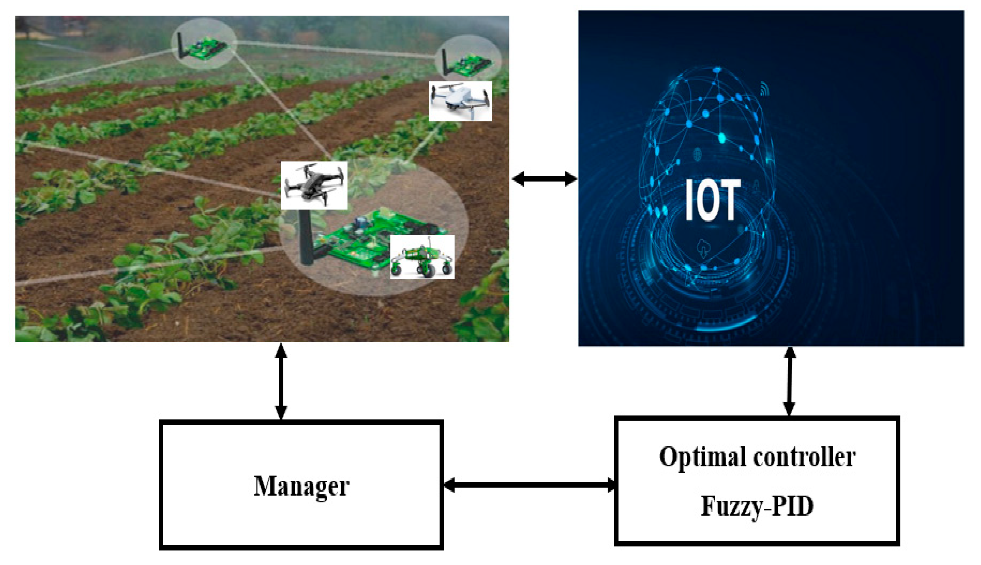
3.1. The Working Principles of Aerial Vehicle Guided Agriculture System

The information flows from the aerial vehicle (drone) to the agriculture manager (Figure 1). The flow of information occurs with the help of the Internet of Things. The IoT enables precision farming, which involves using data to make informed decisions about crop management. This includes optimizing fertilizer application, irrigation, and pest control. From the Internet of Things device, the aerial vehicle captures the status of the agriculture system. The micron troller helps to send the status of the soils to the drone. Before the information flows, the aerial vehicle is made stable with the help of fuzzy PID controllers (optimal fuzzy PID controllers). A fuzzy logic controller uses the outputs of the aerial vehicle parameters as an input. Based on the provided input aerial vehicle parameters, the fuzzy logic controllers’ statements (on/off) are then used as the input for the PID controllers.. This process is cyclically repeated.

3.2. Mathematical Modeling of Quadcopter Motion

The orientation of a rigid body in a coordinate system can be characterized based on the three Euler angles, which can also be used to translate a point’s coordinates from one reference frame to another and to explain the relationship between two reference frames [32,33,34,35]. The Euler angles, which show how a body rotates around the axes of a coordinate system, are represented by the symbols for the roll, pitch, and yaw angles. The position of a quadcopter body is described by six coordinates that are divided into two reference frames. The x, y, and z coordinates, in the cardinal directions of north, east, and down, represent the initial reference frame, which is the fixed coordinate system known as the inertial or Earth frame. The ϕ, θ, and ψ angles with respect to the body’s center of gravity represent the body frame, a movable coordinate system that serves as the second reference frame. The quadcopter has four inputs and six outputs, making it an underactuated nonlinear system [36]. By giving one rotor (or two neighboring rotors) more thrust and the diametrically opposed rotor less thrust, a quadcopter can change its pitch or roll (Figure 2). The thrust force ( T l , T b , T f , T r ) is the force that propels a drone forward. It is generated by the rotation of the drone’s propellers. The weight (mg) of a drone due to gravity is determined by its mass and acceleration due to gravity. Torque   ( τ l , τ b ,   τ f , τ r ) is a measure of the force that causes a drone motor to rotate. In drones, torque is generated by the motors that power the propellers. The amount of torque produced by a motor is determined by its speed and the size of its propeller. Drones use a variety of mechanisms to balance momentum ( M l , M b , M f , M r ) , including propellers, rotors, and wings. By carefully controlling the speed and direction of these components, drones can achieve stable flight and maneuverability.
In the present analysis, the quadcopter was modeled based on the following assumptions in order to reduce the complexity of the system.
The structure is rigid
The structure is axis-symmetrical
The center of gravity and the body-fixed frame origin coincide
The propellers are rigid
Trust and drag are proportional to the square of the propeller’s speed.
The three angles that Leonhard Euler devised to characterize the orientation of a rigid body in a coordinate system are referred to as the Euler angles. They can be used to translate a point’s coordinates from one reference frame to another and to explain the relationship between two reference frames. The Euler angles, which show how a body rotates around the axes of a coordinate system, are represented by the symbols ϕ ,   θ , and ψ for the roll, pitch, and yaw angles, respectively [37,38,39,40]. The three fundamental Euler angles can be combined to achieve any orientation for a rigid body. The following equation gives the rotation matrices, were, c ϕ = c o s ϕ ,   s ϕ = s i n ϕ ,   c θ = c o s θ ,   s θ = s i n θ ,   c ψ = c o s ψ ,   s ψ = s i n ψ :
R x θ = 1 0 0 0 c θ s θ 0 s θ c θ R y = c ϕ 0 s ϕ 0 1 s ϕ s ϕ 0 c ϕ R z ψ = c ψ c ψ 0 s ψ c ψ 0 0 0 1
The rotation matrix depicting the relationship between the inertial frame and the body frame is as follows:
R = R z ψ × R y θ × R x ϕ
R = c θ c ψ s ϕ s θ c ψ   c ϕ s ψ c ϕ s θ c ψ +   s ϕ s ψ c θ s ψ s ϕ s θ s ψ +   c ϕ c ψ c ϕ s θ s ψ   s ϕ c ψ s θ s ϕ c θ c ϕ c θ
where the rotational matrix R is orthogonal, such that
R 1 = R T
The reference frame transformation   x   y   z   ϕ   θ   ψ   T was assumed to be a vector of linear and angular positions in the inertial frame and u   v   ω   p   q   r   T was assumed to be a vector of linear and angular velocities in the body frame. Typically, the derivative gain of angular positions should give angular velocities, but the angular positions and velocities above are in a different frame. The following transformation matrix was used to convert from one reference frame to another:
ζ = x   y   z   T η = ϕ   θ   ψ   T V I = x ˙ y ˙ z ˙ T ω I = ϕ ˙ θ ˙ ψ ˙ T V B = u v ω T ω B = p q r T V I V B ,   a n d   ω I   ω B V I = R . V B ,   ω I = ω η 1 . ω B
ϕ ˙ θ ˙ ψ ˙ = 1 s ϕ t θ c ϕ t θ 0 c ϕ s ϕ 0 s ϕ c θ c ϕ c θ p q r
p q r = 1 0 s θ 0 c ϕ   s ϕ c θ 0 s ϕ c ϕ c θ ϕ ˙ θ ˙ ψ ˙
In rotational motion,
I ω B ˙ + ω B × I ω B   + Γ = τ B
The quadcopter has a symmetrical structure with the four arms aligned with the body’s x- and y-axes. Therefore, the inertia matrix I is a diagonal matrix in which I x x = I y y ,
I = I x x 0 0 0 I y y 0 0 0 I z z
Gyroscopic forces Γ are caused by the combined rotation of the four rotors and the quadcopter body,
Γ = i = 1 4 J r ω B Λ e 3 ^ 1 1 + i ω r i
where
Γ = J r ω B ω r ω r = ω 1 + ω 2 ω 3 + ω T = τ ϕ τ θ τ ψ T
When
i = 2 i = 4 τ ϕ = r x T = l   k t ω 2 2 +   k t ω 4 2   = l k t ω 2 2 +   ω 4 2
τ θ = r x T =   l   k t ω 1 2 +   k t ω 3 2 = l k t ω 1 2 +   ω 3 2  
τ ψ = 1 1 + i k b ω i   2 + I m ω i ˙
where 1 1 + i   1 is positive for the ith propeller if the propeller is spinning clockwise and negative if it is spinning counterclockwise, at steady state ω i ˙   0 , τ ψ = k b ω 1 2 + ω 2 2 ω 3 2 + ω 4 2   , where k t is the thrust coefficient, k b is the drag coefficient, and l is the distance between the rotor and the center of mass of the quadcopter,
T B = τ φ τ θ τ ψ = l k t ω 2 2 +   ω 4 2 l k t ω 1 2 +   ω 3 2 k b ω 1 2 + ω 2 2 ω 3 2 + ω 4 2
Using Newtonian equation to model the linear dynamics, the extraneous forces acting on the quadcopter are:
m V ˙ I = 0 0 m g + R T B + F D
where F D is the drag force acting on the system as a result of fluid friction (air resistance). A simplified equation can be used where F D is friction. Drag force is assumed to be proportional to the linear velocity in all directions, F D = k d V I . The angular velocity of the ith rotor creates a force Fi in the direction of the rotor axis (z-direction). The combined forces create thrust T in the direction of the body’s z-axis:
T = i = 1 4 F i = k t i = 1 4 ω i 2
Since it acts in the z-axis,
T B = 0 0 T = k t 0 0 i = l ω i 2
and
ω B ˙ = I 1 p q r x I x x p I y y q I z z r J r p q r ω r + τ B
p ˙ q ˙ r ˙ = I y y I z z I x x q r I z z I x x I y y p r I x x I y y I z z q p J r q I x x p I y y 0 ω r + τ ϕ I x x τ θ I y y τ ψ I z z
From the linear dynamics,
X ¨   Y ¨   Z ¨ = g 0 0 1 + T m c ψ s θ c ϕ + s ψ s ϕ s ψ s θ c ϕ + c ψ s ϕ c θ c ϕ 1 m k d x 0 0 0 k d y 0 0 0 k d z x ˙ y ˙ z ˙
Once we had developed this mathematical model, the next step was to construct a suitable controller. The challenge for the controller was to read a sensor, process variables in quadcopter control systems, and generate a control signal to dynamically reduce the difference between the output and the desired setpoint of the quadcopter system. The controller model we developed achieves this by computing the PID responses and summing these three components to compute the desired actuator output.

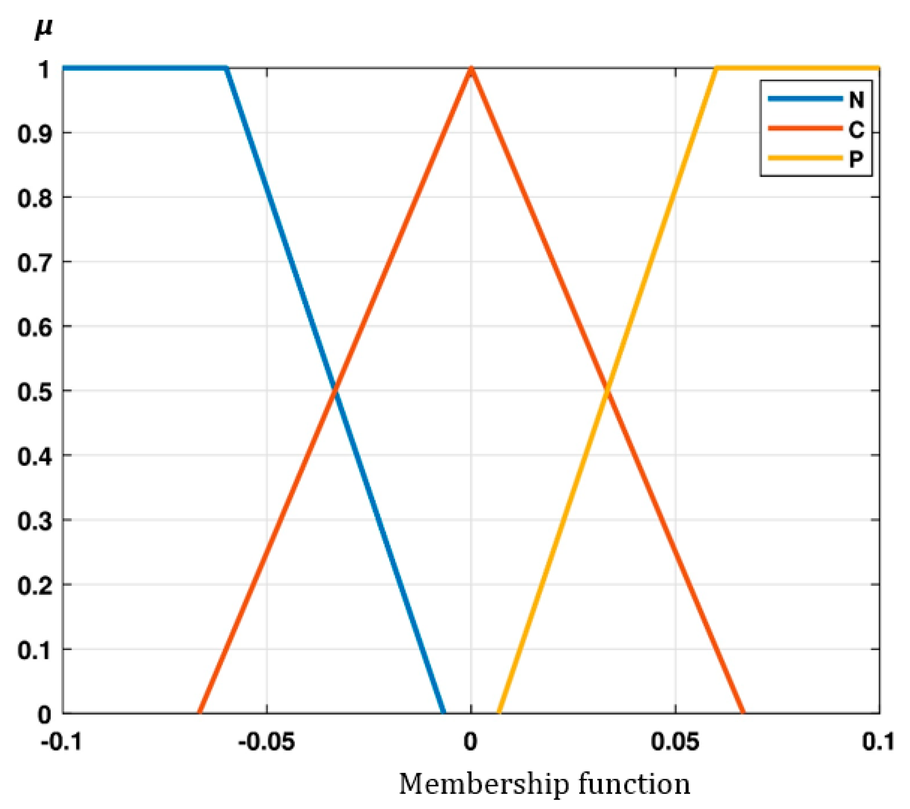
3.3. Control Design for Quadcopter System Stabilization using Fuzzy PID

Manual tuning cannot lead to suitable optimal tuning, but the fuzzy PID tuning method automatically adjusts model parameters against a physical object, which leads to suitable optimal tuning. To overcome this, a fuzzy PID-tuned control design for a quadcopter controller was developed. An aerial vehicle flight test mimicked cruising flight conditions, with adjustments made to the pitch and yaw axes [41]. From Figure 3, it is understood that the output of the fuzzy logic controller is used as an input for the PID controller. The nonlinear PID controller optimizes the plant system-based fuzzy logic outputs. The outputs of the plant are provided for the fuzzy logic controller. Based on the plant feedback system, the fuzzy members on or off, and the results of the fuzzy are provided to the PID controller. The controller has two loops: the inner loop and the outer loop. The inner loop penalizes the PID gain, whereas the outer loop penalizes the fuzzy membership functions. The inner loop consists of a PID controller, whereas the outer loop consists of a fuzzy logic controller.
A quadcopter has only four control inputs and six primary outputs of interest x   y   z   ϕ   θ   ψ , which makes it an underactuated system. This was resolved by creating two different control loops, one working with attitude states and the other with position states. The quadcopter’s angular motion is independent of the linear components, but the linear motion is determined by the angle variables. As a result, the goal was to control the attitude variable, which is independent of the linear motion, and then control the linear motion. It is possible to integrate attitude control with the trajectory controller once it is designed and optimized. The control architecture to be implemented on the quadcopter system was as follows [15,16,17,18,19]:
e t = r t y t
u t = K P e t + K I 0 t e τ d τ + K D   d d t   e t
where u(t) represents the control input, r(t) represents the desired state, and y(t) is the current or actual state. K P ,   K I ,   and   K D are the gain parameters for the proportional, integral, and derivative gains of the PID controller, respectively. Proportional and derivative gains were used for quadcopter control. The torque generated is proportional to the angular velocities, and therefore we set the torques to be proportional to the controller output, such that τ   = I   ×   u t :
τ φ τ θ τ ψ = I xx k P ϕ φ d e s i r e φ + k D ϕ φ ˙ d e s i r e φ ˙ I yy k P θ θ d e s i r e θ + k D θ θ ˙ d e s i r e θ ˙ I zz k P ψ ψ d e s i r e ψ + k D ϕ ψ ˙ d e s i r e ψ ˙
The input to the quadcopter system is the angular velocity of the rotors. Remember that Equation (15) relates the torque to the square of the angular velocity of the rotors; there are three equations, but four unknowns. For this reason, Euler angles were used to model the quadcopter dynamics, rather than quaternions. Physical singularities also occur due to the limitation of under-actuation in the dynamics of a quadcopter. To allow simplification, the total thrust (T), which affects the acceleration in the z-direction, was set to be equal to mg (constraint enforced to keep the quadcopter flying). Converting this thrust equation to the appropriate reference frame and utilizing a PD to minimize the error in the z-axis gives
T = g + k p z z d e s i r e z + k D z z ˙ d e s i r e z ˙ m c ϕ c θ
and then angular velocity becomes
ω 1 2 ω 2 2 ω 3 2 ω 4 2 = k t k t k t k t 0 l k t 0 l k t l k t 0 l k t 0 k b k b k b k b 1 T τ φ τ θ τ ψ
After some simplifications,
ω 1 2 = T 4 k t τ θ 2 l k t τ ψ 4 k b ω 2 2 = T 4 k t τ ϕ 2 l k t + τ ψ 4 k b ω 3 2 = T 4 k t + τ θ 2 l k t τ ψ 4 k b ω 4 2 = T 4 k t + τ ϕ 2 l k t + τ ψ 4 k b
Feedback linearization is a nonlinear control technique where the main concept consists of mathematically converting nonlinear system dynamics into (fully or partially) linear dynamics, allowing linear control methods to be used. Our goal was to design a controller that could exactly cancel out the system dynamics. From Equation (10), we replaced x ˙ = k Dx k x x   x d , x ¨ = k px k x x ˙ x ˙ d , where k p x ,   k D x , and k x are gain values, and replaced y ¨ ,   y ˙ ,   z ¨ , and z ˙ , respectively:
T m c ψ s θ c ϕ + s ψ s ϕ s ψ s θ c ϕ + c ψ s ϕ c θ c ϕ = k px k x x ˙ x ˙ d k py k y y ˙ y ˙ d k pz k z z ˙ z ˙ d + g 0 0 1 + 1 m k Dx k x x     x d k Dy k y y     y d k Dz k z z z d
Back substituting Equation (17) into Equation (15) gives
k px k x x ˙ x ˙ d + k D x k x m x x d = T m c ψ s θ c ϕ k py k y y ˙ y ˙ d + k D x k x m y y d = T m s ψ s θ c ϕ + c ψ s ϕ   k pz k z z ˙ z ˙ d + k D x k x m z z d = T m s ψ s θ c ϕ + c θ c ϕ    
Taking the square of both sides of Equation (18) and adding the equations together gives
T 2 m 2 =   k p x 2 x ˙ x ˙ d 2 + k D x 2 k x 2 m x x d 2 + 2 k p x k x k D x m x x d x ˙ x ˙ d + k p y 2 y ˙ y ˙ d 2 + k D y 2 k y 2 m y y d 2 + 2 k p y k y k D y m y y d y ˙ y ˙ d + k p z 2 z ˙ z ˙ d 2 + k D z 2 k z 2 m z z d 2 + g 2 + 2 g k a z z ˙ z ˙ d + 2 g k D z k z m z z d + 2 k p z k D z k z m z z d z ˙ z ˙ d
From Equation (16),
F x = c ψ s θ c ϕ + s ψ s ϕ F y = s ψ s θ c ϕ c ψ s ϕ
and from the equation
s θ c ϕ = Fy   +   c ψ s ϕ   s ψ
F x = c ψ s ψ F y + c ψ s ϕ + s ψ s ϕ   s ϕ = F x F y l t ψ   c ψ +   s ψ t ψ lt ψ s ϕ = F x t ψ   F y c ψ +   s ψ t ψ d = sin 1 F x tan ψ   F y cos ψ + sin ψ tan ψ θ d = tan 1 F x cos 2   ψ F y sin ψ cos ψ F z cos ψ
This study optimizes controller design for agricultural drones by identifying a suitable penalty rate gain, understanding constraints, and drawing conclusions. It develops a design technique based on fuzzy PID control law, digitalizing traditional PID control law for modern applications and utilizing feedback for gain regulation [35,36,37,38,39].
t c m d = K P e t + K I e t K D e t
where e t = r t y t is the tracking error signal between the reference r(t) and the controlled system output, y t , and K P ,   K I , and K D are constant P, I, and D gains respectively. This is first converted into the frequency domain to obtain
U S c m d = K P E S + K I E S S + K D S E S
and the associated Laplace transform is denoted by the capital variable. The bilinear transform can then be used to transfer this equation into the discrete-frequency domain with the variable z. S = 2 T 1 Z 1 1 + Z 1 , where T > 0 is the sampling period, and E(Z) substitutes SE(S), to produce
U Z c m d = K P E Z + K I T 21 + Z 1 1 Z 1 E Z + K D E Z
Eliminating the denominator yields
U Z c m d 1 Z 1 = K P E Z 1 Z 1 + K I T 2 1 + Z 1 E Z + K D E Z 1 Z 1
This equation can be converted back to the discrete-time domain using the inverse z transformation to produce
u n T c m d u n T T c m d = K p ( e n T e n T T ) + K I T 2 ( e n T + e n T T ) + k D ( e n T e n T T )
where n = 0 , 1 , 2 , . By rearranging terms, collecting like terms, and then substituting the terms
K P = K P T K I = K I T
we obtain
u n T c m d = u n T T c m d + K I e n T + K p ( e n T e n T T ) + k D ( e n T e n T T )
A unique fuzzy logic version of Equation (40) will be developed for reliable system controllers, providing direct behavior insight and analytic structures for the easy prediction of actions, requiring good general rules. The fuzzy PID control is developed from traditional PID. Based on the fuzzy control theory, the fuzzy relationship between the three PID parameters K P ,   K I ,   and   K D and the error e and error change rate e z can be established. According to different e and e z , the parameters K P ,   K I ,   and   K D can be self-adjusted online in order to ensure that the controlled object has good dynamic and static performance, meeting different control requirements. In general, fuzzy control has no knowledge database, does not have adaptive ability, and its flexibility and interactivity are not very good. Contrarily, automatic-tuned systems often cannot be directly used to control objects or production processes. So, the combination of fuzzy PID and automatic-tuned control will bring their respective advantages into play. Four controllers generated the control signals, which the method used directly z ,   ϕ ,   θ ,   ψ . On the other hand, the remaining torques U x   and   U y allows the calculation of the reference pitch and roll angles, which, together with the control signals, will enable the system to follow the desired trajectory. The z-variable controller regulates the height of the Hex rotor. The output of this controller returns the total power required by the rotors to correct the error. The difference in the desired altitude causes this error compared to the actual altitude of the Hex rotor [42,43].
e z = z r z ,
taking the time derivative for Equation (41), then the new equation becomes
e z ˙ = z r ˙ z ˙
These variables can be used to create a fuzzy controller for the UAV’s z-axis. Three functions of membership, namely a negative input (N), an input in a range near zero (C), and a positive input (P), were employed for this controller in order to represent the height error and its derivative. Initially, in order to fuzzify the data, each input variable was given a degree of membership with respect to the membership functions that were previously established in the fuzzy sets. Second, nine member functions were used to define the output variable, ranging from the most negative (NNNN) to the most positive (PPPP). The membership functions of the triangular and trapezoidal types were selected. When there is an ideal central value, which is lost when it is far from the center, the triangular and trapezoidal form are suitable. Conversely, structures with a range of ideal values use the triangular and trapezoidal function. For the central values in this instance, the triangular and trapezoidal function was appropriate, and for the extreme values, the triangular and trapezoidal functions were used.
The arithmetic mean or average position of all the points in the shape could be obtained [44].
C = μ x = g x . x . d x g x d x  
The magnitudes of the expected errors in the linear and angular positions and their derivatives were used to choose the values of the universes. As a result, various worlds were chosen based on the controlled axis. The X and Y controllers used the range of −0.5 to 0.5 m. The universe in the ϕ ,   θ ,   and   ψ angle controllers was −90 to 90 degrees to cover the full range of angular motion. Finally, minor variations in the error are expected in the Z-axis [45]. Thus, its universe varies from −0.1 to 0.1 m. The maximum expected rates of change were used to select the range in derivative inputs. After defining the inputs and outputs of the control system, it was necessary to dictate the rules that govern its behavior. The set of rules shown in Table 1 were designed for this. In addition, the Mamdani-type fuzzy inference system and a defuzzification based on the centroid method were used [46].
The input membership functions are presented in Figure 4. The blue line indicates the negative input, the red line indicates the input close to zero, and the yellow line represents the positive input.
The output membership functions are presented in Figure 5, and the most negative (NNNN), the most negative (NNN), more negative (NN), negative (N), close to zero (C), positive (P), more positive (PP), most positive (PPP), and the most negative (PPPP) are represented by blue, maroon, yellow, purple, green, dark red, turquoise, and red, respectively.
Fuzzy reasoning and defuzzification.
According to the fuzzy tables, we can obtain 81 × 2 fuzzy rules and they can be described using the following statements. If e = A i and if e z = B j , then K p K i , K d = C i j , where A i ,   B j   and   C i j are the fuzzy sets of the error E, the error change rate EC and PID parameters K p ,   K i ,   and   K d respectively. So, the membership function of R is u R X , Y , Z = u A i X   u B j   Y   u C k Z , and the following expression of the PID parameter K p can be given as u k p Z = u R X ,   Y , Z   u B j   Y   u C k Z .
Consequently, the output of K p is as follows:
K p = j = 2 j = 2 j . u k p j j = 2 j = 2 u k p j
Finally, we arrived at
U F u z z y P I D t = K p F u z z y P I D e t + K I F u z z y P I D 0 t ( K I F u z z y P I D e t ) d t + K D F u z z y P I D d e t d t

3.4. Quadcopter Path Planning Assistance System

Traverse planning ensures smooth quadcopter system operation, and motion planning makes the quadcopter intelligent. This analysis focuses on quadcopter dynamics, studying motion while considering force or torque, recalling Figure 2. Continuous first and second derivatives of angular displacement and acceleration are necessary for smooth system variation over time.
If the position is known in the Cartesian coordinate system, then solving the inverse kinematics provides two sets of orientation values. The DC motor of the quadcopter must therefore produce this particular angular displacement. In order to control the motor, the only option is to utilize the quadcopter scheme (Table 2). To ensure smooth variation in theta during a particular cycle time, the controller has to feed a smooth curve passing through θ 1 s , θ 1 1 ,   θ 1 2 ,   θ 2 3 ,   and   θ 1 G . Similarly, it will have to find out another smooth curve for θ 2 s ,   θ 2 1 ,   θ 2 2 ,   θ 2 3 ,   and   θ 2 G , the smooth variation of θ 2 .
Consider the case polynomial trajectory plan,
t = t i = 0 , t = t f ; θ = θ i θ = θ f θ ˙ = 0  
so that
θ t = C 0 + C 1 t + C 2 t 2 + C 3 t 3
where C 0 , C 1 , C 2 ,   and   C 3 are coefficients. Differentiating θ t with respect to time gives the angular velocity:
θ ˙ t = C 1 + 2 C 2 t + 3 C 3 t 2
Applying the initial conditions to angular displacement and the velocity equation C 0 = θ i C 1 = 0 gives:
C 0 + C 1 t + C 2 t 2 + C 3 t 3 = θ f C 1 + 2 C 2 t + 3 C 3 t 2 = 0
Substituting the Equation (30) into Equation (33), we obtain
θ t = θ i + 3 θ f θ i t f 2 t 2 2 θ f θ i t f 3 t 3
Theta is then actually a function of time t, and can be plotted as a trajectory line.

3.5. Characteristics Analyzed for the UAV Response

Settling time ( T S ) , i.e., the time required for the output to stabilize within a given tolerance band, is described mathematically as
T s = 4 σ ω n , 0 < σ < 1   σ = 0   6 ω n σ > 1
where σ is the damped ratio.
The rise time (Tr) describes the time taken for the solution to increase from 0% to 100% of its ultimate value in underdamped systems, or from 10% to 90% of its final value in over-damped systems. Mathematically,
T r = π θ ω d
The peak time (Tp) is the time required for the response to reach the peak value for the first time. Mathematically,
T p = π ω d
The peak overshoot, or maximum overshoot (Mp), is defined as the deviation of the response at the peak time from the final value of response. It is expressed as
M p = e σ π 1 σ 2 100
At the steady state time (Tss), the rate of input is equal to the rate of elimination.

3.6. Theoretical Analysis of the Proposed Results: Lyapunov Stability Criteria for Agricultural Drones

Drone systems for agriculture are among the many dynamical systems whose stability can be examined using the robust Lyapunov stability criterion. This criterion is utilized in control system design to guarantee that the agricultural drone system is stable throughout operation. We assume the difference between y and the steady state. If that reaches zero, then the state space is stable. If it increases, and if y moves further away from the steady state, it is unstable. We pick a (non-negative) function such that the value decreases along the trajectory of the agricultural drone. Consider a mass (m) acted on by a dissipative force as
m x ¨ = b x ˙
where m is mass of the agricultural drone and b is the air drag friction coefficient.
This implies that
m v ˙ = b v
where v is the speed of the agricultural drone.
X = 0 , v = 0 at equilibrium points.
The kinetic energy could be
E t = 1 2 m v 2  
and its derivative could be
E ˙ t = m v . v ˙ = b v 2 < 0
Since E t 0 and E ˙ t < 0 , E t is positive, zero, and decreasing E t 0 , as t . This implies that v t 0 , as t . To make this more abstract, we pick a non-negative scalar function ( v x ) that decreases along the trajectories of the agricultural drone, namely x ˙ = f x .
v ˙ x = i = 1 v x i x i ˙ = i = 1 n v x i f x = v x . f x
If v x . f x < 0 , v x . f x > 0 ,   and   v x , f x = 0 , then the function is inwards, perpendicular, and away, respectively, with respective to the level sets of v x . That means that the level sets are positive invariants. Therefore, stability in the sense of the Lyapunov law is summarized as follows.
Let x = 0 be an equilibrium point of x ˙ = f x and let v(x) be a continuously differentiable function. If v x = 0   and   v x > 0   for   x 0 , and if v x 0 ,   then the system ( x ) is stable at the equilibrium points. This implies the the system ( x ) with a fuzzy PID controller provides stability for agricultural drones.
If v ˙ x < 0 , then the system ( x ) is asymptotically stable at the equilibrium points. If v ˙ x 0 and v ˙ x = 0 , only at x = x , this implies that the system ( x ) is asymptotically stable at the equilibrium points. This indicates that the PID controller provides asymptotic stability for agricultural drones. In this instance, the Lyapunov stability proof offers a method to quantitatively prove the stability of a dynamical system for agricultural drones. Finding a function known as the “Lyapunov function” that becomes less valuable as the system deviates from its equilibrium state is the goal. This suggests that the agricultural drone system is stable because it tends to revert to equilibrium. Therefore, the proposed controllers were the most suited to stabilizing agricultural drones during their operation in agricultural fields.

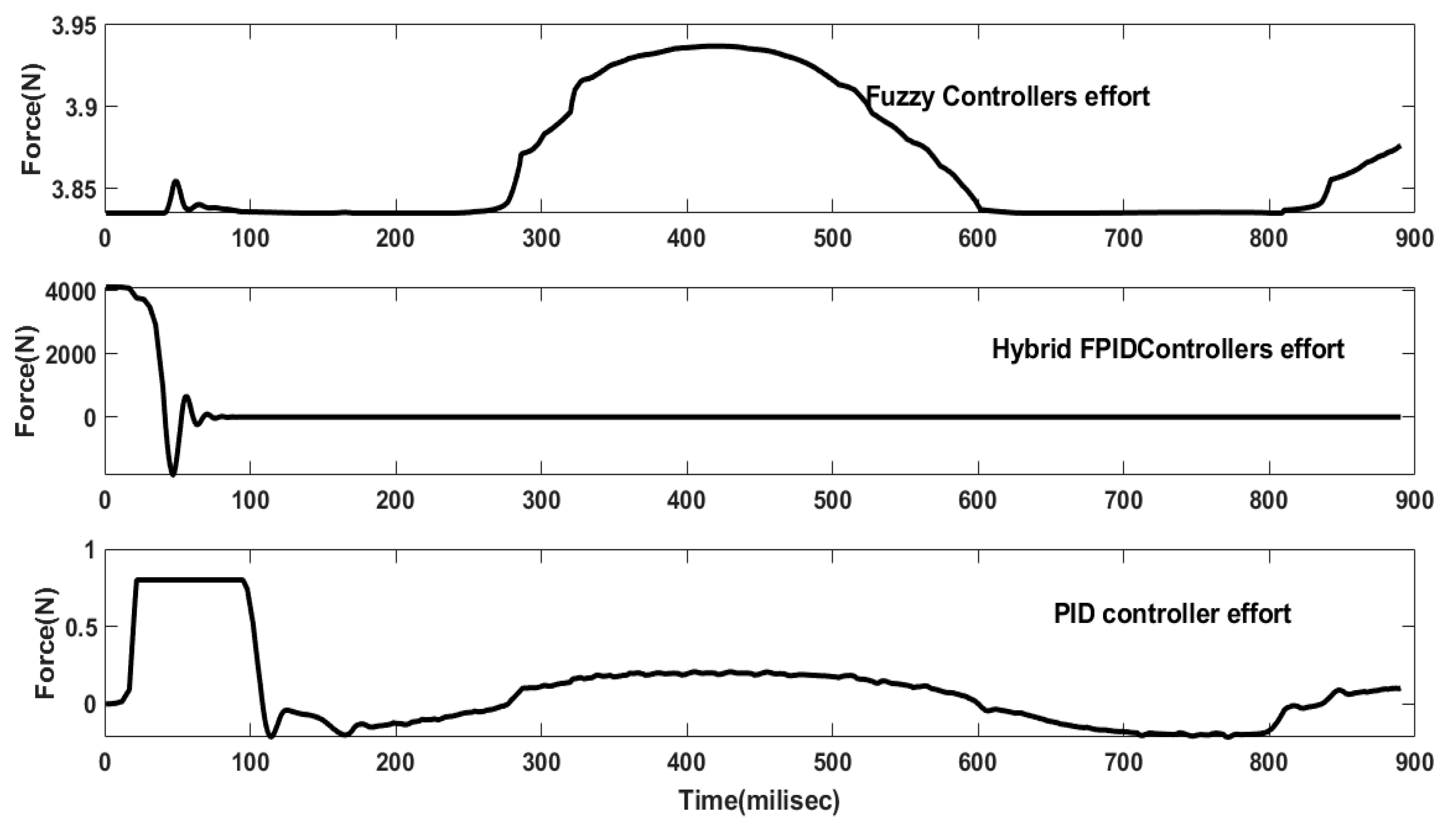
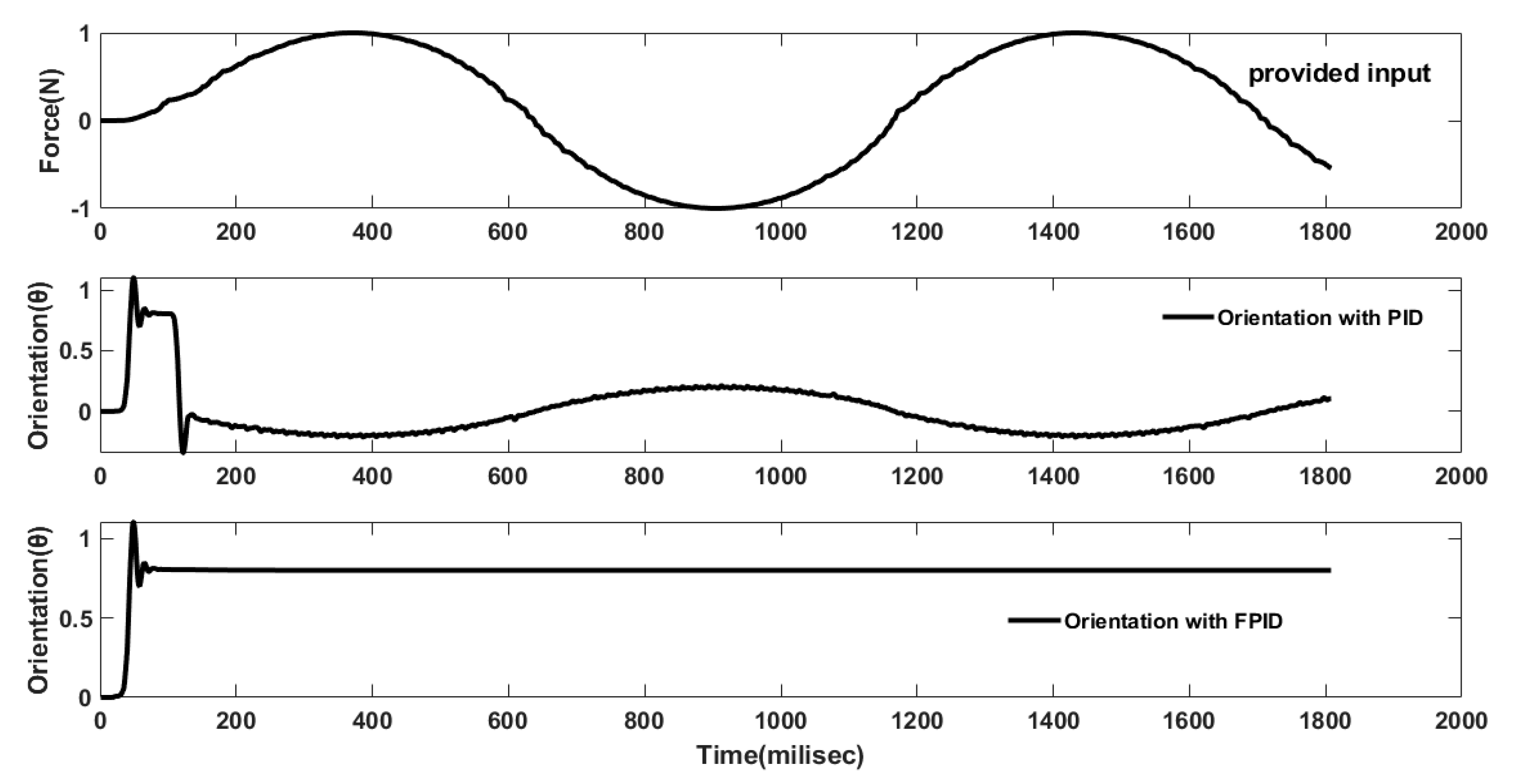
4. Results and Discussion

Figure 6 illustrates the fuzzy logic controller’s effort in agricultural drones, which involves designing, implementing, and maintaining a controller. Fuzzy PID controllers use fuzzy logic to generate decisions, which are then inputted into a PID controller. The size, complexity, inputs, outputs, and performance of the system affect the design effort. The fuzzy logic controller’s effort allows for the representation and manipulation of imprecise or uncertain information, allowing for a more nuanced representation of the system. It uses a PID controller in agricultural drone systems to modify the output based on discrepancies between the intended and actual output. The fuzzy logic PID controller can be used for regulation and optimization, with hybrid controllers being the most stable and error-free option. Hybrid controllers are stable over time and have fewer errors than individual PID controllers. The magnitude of the horizontal axis for all controller efforts was the same, but the magnitude of the vertical axis was different. The reason for this is that the force required by the PID controller to stabilize the UAV system is much smaller than the force required by the fuzzy PID controller. Since fuzzy PID controllers used huge energy to push the UAV system, it suddenly returned to its original position. Although the amount of force required by the PID controller was small, it was unable to return the UAV system to its initial position. Fuzzy PID controllers have improved accuracy and efficiency, especially in systems with non-linear dynamics. The reduced overshoot and settling time, resulting in a faster and more stable system response and enhanced robustness to parameter variations and disturbances, make the system more resilient to changes in operating conditions. The force required by a fuzzy controller is less compared to that required by a hybrid controller and more than that required by a PID controller. Because a fuzzy logic controller is compared to a fuzzy PID controller, fuzzy logic controllers can be more complex to design and tune. Fuzzy logic controllers typically require more expertise and effort to determine the appropriate fuzzy sets, membership functions, rules, and defuzzification methods. On the other hand, fuzzy PID controllers combine the advantages of classical PID controllers with the flexibility of fuzzy logic, offering a more structured and familiar framework for control system design and tuning. Additionally, fuzzy PID controllers can provide better performance in certain applications by incorporating the benefits of both fuzzy logic and PID control. All of the results were plotted until the final time frame, but due to PID controllers, the horizon became wide. As the optimal gain approached the exact controller gains, the horizon became wider. Any gains around the optimal controller are also applied to the UAV system.
Figure 7 illustrates the nonlinear wave function that is used as the input for the agricultural drone. While time is displayed in milliseconds, the vertical axis is measured in force (N). Based on the input given, it was found that the agricultural drone’s location was aligned the same using both fuzzy PID and PID controllers. There is consistency among them all. This suggests that the hybrid farm drone (fuzzy PID) controller performs similarly to the PID controller in terms of effort position.
Conversely, given the identical input, there is a divergence in the case of the agricultural drone’s orientation (Figure 8). More work is completed with hybrid (fuzzy PID) controllers than with standalone PID controllers. This is because the agricultural drone system has elements of both the PID controller (which lowers error) and the fuzzy logic controller (which is more resilient to noise and disturbances). Because of this, the agricultural drone’s orientation is established with the least amount of time needed. On the other hand, the agricultural drone orientation takes longer to get used to. When comparing the orientation of an agricultural drone packed with a fuzzy PID and a PID controller, the former takes less time to settle, more quickly reaches overshoot, is smoothest after reaching the settlement time, and does not have a global minimum. On the other hand, the latter takes more time to settle, more slowly reaches overshoot, chatters after reaching the settlement time, and has a global minimum.
Both the fuzzy PID and PID controllers’ performance with regard to the agricultural drone system can be seen in Figure 9. When compared to the farm drone controlled using a PID controller, the drone controlled using a fuzzy PID controller performed better at a given velocity with the same input. The obtained results suggest that the agricultural velocity with the hybrid fuzzy PID controller takes less time to settle, achieves overshoot faster, and has a smoother trajectory after reaching the settlement time. In contrast, the agricultural velocity using a PID controller has two global maximum points and is cyclically stable over time.
The errors resulting from the drone performance in agriculture are shown in Figure 10. These errors were acquired by subtracting the PID controller from the agricultural drone system with a fuzzy PID controller. Positional errors rose to a predetermined value before stabilizing at the lowest possible value. While there appears to be less noise throughout the orientation portion of the performance than during the velocity portion, the position appears to be dynamic throughout. Because the hybrid and individual controllers operate similarly, the position case becomes smooth. In contrast, the error is not smoother prior to the orientation performance, since the hybrid and individual controller performances deviated.
The test results of the fuzzy, fuzzy PID, and PID controller efforts at the noise input are shown in Figure 11. The maintenance effort for a fuzzy logic controller alone (fuzzy controller effort) is usually less than that of a conventional control system. This is due to the fact that fuzzy logic controllers are less susceptible to changes in the system they are controlling and are more resilient. Because it shares some advantages with fuzzy logic controllers, such as being more efficient than traditional control systems, and with PID controllers, such as eliminating steady-state errors and minimizing overshoot and oscillations, the hybrid controller’s effort becomes smooth throughout the performance. Only the PID controller revealed some system-wide noise. This is due to the possibility that in complex systems with highly nonlinear dynamics or large time delays, controllers may find it difficult to deliver optimal control performance. The agricultural drone continued to operate as intended, with the fuzzy logic algorithm adjusting the issues based on feedback.
The input given was noise, as seen in Figure 12. The fuzzy PID (hybrid) and PID controllers’ performance with regard to the agricultural drone was obtained based on the input given. The performance of the position remained constant throughout, since there was no difference in the strength of the controller response to an input or output signal deviation. The controller gain for an agricultural drone in a control loop is the amount of action a controller will take at a specific point (position) below or above the setpoint.
Figure 13 depicts the varied performance for the orientation of the farm drone.
The agricultural drone’s PID controller does not make the system’s orientation any smoother. PID controllers may cause instability or subpar control performance because they are susceptible to noise in the measurement or control signals. PID controller parameter tuning can be difficult, particularly for systems with complicated dynamics. Control engineering knowledge and experience are needed for this task. However, the system’s overall performance was smooth when using a fuzzy PID controller for drone orientation. This is because fuzzy PID controllers have a number of benefits over conventional control systems, such as efficiency, adaptability, and resilience.
Figure 14 shows the agricultural drone’s velocity response. The agricultural drone that has a PID controller exhibits cyclical stability in its velocity, while the drone outfitted with a fuzzy PID controller displays steady velocity. The agricultural drone’s velocity may be readily adjusted to various operating conditions thanks to its fuzzy PID controller, which also requires less processing. These traits are common to fuzzy logic controllers. The agricultural drone’s velocity with the fuzzy PID controller has a smooth form, it is quick to achieve its maximum points, it overshoots, it settles quickly, and it may readily obtain a steady-state error. The agricultural drone’s PID controller-equipped velocity has a less smooth shape and is cyclically stable. Because PID controllers do not specifically take into account system constraints, including input or output limits, breaking these constraints could result in unfavorable behavior. The fuzzy PID technique balanced this controller effort. Because of this, fuzzy PID controllers can perform better in control than conventional PID controllers, particularly in systems that have uncertainties and non-linearities.
Figure 15 displays the inaccuracy. This was calculated by deducting the performance of the PID controller from that of the FPID controller. The position error increases positively and is smooth, because an agricultural drone’s position is affected by both PID and FPID controllers in the same way. On the other hand, orientation issues are a talking point, since the position of the agricultural drone indicates that the FPID and PID controllers have different effects.
The agricultural drone’s ability to follow the course is evaluated once the controller design is complete. Given that a device labeled as an agricultural drone path tracking controller assists drones in following an established path, the agricultural drone’s position and orientation are usually measured by sensors, and the necessary control inputs are then computed based on these data to maintain the drone’s trajectory. Path tracking controllers can be utilized by agricultural drones to adhere to pre-established routes, like those generated using waypoints or GPS locations, as illustrated in Figure 16. The agricultural drone can track along the designated path with almost no errors, according to Figure 16, due to the fuzzy PID controllers.
Figure 17 shows two-dimensional path tracking. The agricultural drone’s track for is shown as a blue line along the horizontal axis and a red line along the vertical axis. In the graphs, the black and yellow dots indicate the obstacle, while the green dot shows the agricultural drone’s moment. The drone’s guided path is indicated by a red arrow in the curve. Agricultural drones can employ route tracking controllers to avoid obstacles like trees, buildings, and other objects in agricultural areas. The agricultural drone in this study is correctly tracked on a particular path. This drone can additionally fly in formation using route tracking controllers, which is helpful for jobs like pest control, aerial photography, and search and rescue missions. Generally, fuzzy PID controllers guide the correct path tracking for agricultural drones.
All tabulated results were obtained automatically, which means that automatic PID tuning is the process of tuning controller gains based on a plant model (plant data). We used Simulink Control Design for tuning PID gains in a Simulink model. The fuzzy function adjusts PID parameters during the auto-tune cycle to enable the process to reach a predetermined setpoint in the shortest time with minimum overshoot and undershoot during power-up or load disturbances.
Table 3 shows the step change parameters: a roll angle of 30°, a height of 5 m, and an airspeed of 1 meter per second, respectively. The PID controller improvements were as follows: proportional, 5.4448; integral, 0; and derivative, 4.6668. The low-fidelity (within 2%), medium-fidelity (within 2%), and high-fidelity (within 2%) responses for the roll angle with the auto-tuned controller represented 41.5%, 41.5%, and 41.5% improvement compared with the compensator, respectively. For the height or altitude of the quadcopter position, the corresponding low-, medium-, and high-fidelity responses for the automatically tuned controller compared with the manual compensator were 11%, 11%, and 17.4%, respectively, while for the quadcopter’s airspeed, they were 44%, 2%, and 2%, respectively. These improvements show that the automatically tuned controller was the better option.
The roll for the drone in low, medium, and high fidelity is compared to the current work parameters (Table 4), which are 35.31%, 39.45%, and 53.6%, respectively, over the prior research work parameters. The present work parameters are 7%, 7%, and 8%, respectively, higher than the previous study’s work parameters for the drone’s height in low, medium, and high fidelity. In comparison to the previous study’s work parameters, the drone’s airspeed in low, medium, and high fidelity is 72.08%, 41.22%, and 43.88%, respectively, under the present work conditions.
Table 5 shows the obtained results of the state characteristic responses. The obtained results indicate a percentage change for the fuzzy PID controller over the PID controller of 90%, 35%, 56.67%, and 72.22% for overshoot, settling time, rise time, and steady state error, respectively. The percentages of change for the fuzzy PID controller over the fuzzy controller were 80% for overshoot, 8.23% for settling time, 33.67% for rise time, and 50% for steady state error. Therefore, combined controller schemes demonstrated the best performances.
Table 6 shows the obtained results concerning PID controllers.

5. Conclusions

This paper was focused on mathematically modeling the dynamics of a quadcopter system using Newton’s and Euler’s laws, a fuzzy PID controller, and its entire system simulation. The model was used to test the fuzzy PID controller’s performance for an agricultural drone system, and the Lyapunov law of stability was applied for the controller stability analysis. The obtained results for the fuzzy PID controller were stable, while the classical PID controller was asymptotically stable. We obtained a quadcopter system with an airspeed rise time of 76.1 s, predicting overshoot if a roll angle signal processing function went over this limit. The system achieved a steady state time velocity of 77.4 s, and its peak time for the roll angle response was 78.4 s. This indicates that the state of the aerial vehicle parameters was effectively stable. The classical PID was far less effective than the fuzzy PID-adjusted controller. With the fuzzy PID controller, the roll angle response with low fidelity (within 2%), medium fidelity (within 2%), and high fidelity (within 2%) displayed, respectively, a 41.5%, 41.5%, and 41.5% improvement compared with the classical PID controller. In comparison to the current work parameters, the roll for the drone in low, medium, and high fidelity is 35.31%, 39.45%, and 53.6%, respectively, better than in the previous research work conditions. This suggests that, compared to earlier studies, the current model performed the best. The simulation results revealed that the fuzzy PID controller outperformed the classically adjusted PID controller. When the fuzzy PID controller was compared with others used in previous research based on the same quadcopter model, it outperformed these significantly, confirming that the controller was appropriately tuned and is appropriate for use with quadcopter systems in agricultural applications. The fuzzy PID system has the best performance compared to classical PID controllers. Therefore, the authors claimed that the performance of the proposed new type of controller algorithms would be suitable for agricultural UAV systems and for an experiment in a real-world environment with a physical UAV. The impacts of the current work will reduce the cost of agricultural activities (time, labor, and capital), improve the efficiency of farming, solve the problem of labor shortages caused by the lack of human labor, prevent the loss and damage of fruits caused by traditional mechanical or manual harvesting, and eventually reduce food waste and loss. For the scientific community, it will expand the application scenarios of combining different controller algorithms and systems and provide integrated control mechanisms and theories for control systems. In addition, new solutions and ideas are being put forward for the problems in agricultural farming. For the business-oriented community, it will transfer knowledge and experience on the topic. It can also boost the development of combining different control schemes. For future work, it is recommended that experiments be carried out on real UAV systems under real operating conditions.

Author Contributions

Conceptualization, S.A.; methodology, S.A.; software, S.A.; validation S.A., formal analysis, S.A.; investigation, S.A.; resources, S.A.; data curation, S.A.; writing—original draft preparation, S.A. and G.G.; writing—review and editing, S.A., G.G. and H.M.A.; visualization, S.A.; supervision, G.G. and H.M.A.; project administration, G.G.; funding acquisition, G.G. All authors have read and agreed to the published version of the manuscript.

Funding

This research received no external funding.

Institutional Review Board Statement

No applicable.

Informed Consent Statement

No applicable.

Data Availability Statement

The data presented in this study are available in article.

Conflicts of Interest

The authors declare no conflict of interest.

References

  1. Idrissi, M.; Salami, M.; Annaz, F. A Review of Quadrotor Unmanned Aerial Vehicles: Applications, Architectural Design and Control Algorithms. J. Intell. Robot. Syst. 2022, 104, 22. [Google Scholar] [CrossRef]
  2. Amertet, S.; Gebresenbet, G.; Alwan, H.M.; Vladmirovna, K.O. Assessment of Smart Mechatronics Applications in Agriculture: A Review. Appl. Sci. 2023, 13, 7315. [Google Scholar] [CrossRef]
  3. Telli, K.; Kraa, O.; Himeur, Y.; Ouamane, A.; Boumehraz, M.; Atalla, S.; Mansoor, W. A Comprehensive Review of Recent Research Trends on Unmanned Aerial Vehicles (UAVs). Systems 2023, 11, 400. [Google Scholar] [CrossRef]
  4. Lee, H.-W.; Lee, C.-S. Research on logistics of intelligent unmanned aerial vehicle integration system. J. Ind. Inf. Integr. 2023, 36, 100534. [Google Scholar] [CrossRef]
  5. Abbas, N.; Abbas, Z.; Liu, X.; Khan, S.S.; Foster, E.D.; Larkin, S. A Survey: Future Smart Cities Based on Advance Control of Unmanned Aerial Vehicles (UAVs). Appl. Sci. 2023, 13, 9881. [Google Scholar] [CrossRef]
  6. Si, X.; Xu, G.; Ke, M.; Zhang, H.; Tong, K.; Qi, F. Relative Localization within a Quadcopter Unmanned Aerial Vehicle Swarm Based on Airborne Monocular Vision. Drones 2023, 7, 612. [Google Scholar] [CrossRef]
  7. Sai, S.; Garg, A.; Jhawar, K.; Chamola, V.; Sikdar, B. A Comprehensive Survey on Artificial Intelligence for Unmanned Aerial Vehicles. IEEE Open J. Veh. Technol. 2023, 4, 713–738. [Google Scholar] [CrossRef]
  8. Cardenas, J.A.; Carrero, U.E.; Camacho, E.C.; Calderon, J.M. Intelligent Position Controller for Unmanned Aerial Vehicles (UAV) Based on Supervised Deep Learning. Machines 2023, 11, 606. [Google Scholar] [CrossRef]
  9. Ganesan, T.; Jayarajan, N.; Shri Varun, B.G. Dynamic Control, Architecture, and Communication Protocol for Swarm Unmanned Aerial Vehicles. In Computing in Intelligent Transportation Systems; Naganathan, A., Jayarajan, N., Bin Ibne Reaz, M., Eds.; Springer International Publishing: Cham, Switzerland, 2023; pp. 31–49. [Google Scholar] [CrossRef]
  10. Din, A.F.U.; Mir, I.; Gul, F.; Al Nasar, M.R.; Abualigah, L. Reinforced Learning-Based Robust Control Design for Unmanned Aerial Vehicle. Arab. J. Sci. Eng. 2023, 48, 1221–1236. [Google Scholar] [CrossRef]
  11. Amin, R.; Aijun, L.; Shamshirband, S. A review of quadrotor UAV: Control methodologies and performance evaluation. Int. J. Autom. Control. 2016, 10, 87. [Google Scholar] [CrossRef]
  12. Li, Y.; Chen, C.; Chen, W. Research on Longitudinal Control Algorithm for Flying Wing UAV Based on LQR Technology. Int. J. Smart Sens. Intell. Syst. 2013, 6, 2155–2181. [Google Scholar] [CrossRef]
  13. Abdelmaksoud, S.I.; Mailah, M.; Abdallah, A.M. Control Strategies and Novel Techniques for Autonomous Rotorcraft Unmanned Aerial Vehicles: A Review. IEEE Access 2020, 8, 195142–195169. [Google Scholar] [CrossRef]
  14. Hoffmann, G.; Huang, H.; Waslander, S.; Tomlin, C. Quadrotor Helicopter Flight Dynamics and Control: Theory and Experiment. In Proceedings of the AIAA Guidance, Navigation and Control Conference and Exhibit, Hilton Head, SC, USA, 20–23 August 2007; American Institute of Aeronautics and Astronautics: Reston, VA, USA, 2007. [Google Scholar]
  15. Hu, X.; Assaad, R.H. The Use of Unmanned Ground Vehicles and Unmanned Aerial Vehicles in the Civil Infrastructure Sector: Applications, Robotic Platforms, Sensors, and Algorithms. Expert Syst. Appl. 2023, 232, 120897. [Google Scholar] [CrossRef]
  16. Ibrahim, I.A.; Truby, J.M. FarmTech: Regulating the use of digital technologies in the agricultural sector. Food Energy Secur. 2023, 12, e483. [Google Scholar] [CrossRef]
  17. James, C.; Chen, G.; Ogmen, H. Fuzzy PID controller: Design, performance evaluation, and stability analysis. Inf. Sci. 2000, 123, 249–270. [Google Scholar]
  18. Praharaj, M.; Sain, D.; Mohan, B. Development, experimental validation, and comparison of interval type-2 Mamdani fuzzy PID controllers with different footprints of uncertainty. Inf. Sci. 2022, 601, 374–402. [Google Scholar] [CrossRef]
  19. Anupam, K.; Kumar, V. A novel interval type-2 fractional order fuzzy PID controller: Design, performance evaluation, and its optimal time domain tuning. ISA Trans. 2017, 68, 251–275. [Google Scholar]
  20. Kumar, A.; Kumar, V. Hybridized ABC-GA optimized fractional order fuzzy pre-compensated FOPID control design for 2-DOF robot manipulator. AEU-Int. J. Electron. Commun. 2017, 79, 219–233. [Google Scholar] [CrossRef]
  21. El-Nagar, A.M.; El-Bardini, M. Hardware-in-the-loop simulation of interval type-2 fuzzy PD controller for uncertain nonlinear system using low cost microcontroller. Appl. Math. Model. 2016, 40, 2346–2355. [Google Scholar] [CrossRef]
  22. Jesus, I.S.; Barbosa, R.S. Genetic optimization of fuzzy fractional PD+I controllers. ISA Trans. 2015, 57, 220–230. [Google Scholar] [CrossRef] [PubMed]
  23. Amertet Finecomess, S.; Gebresenbet, G.; Alwan, H.M. Utilizing an Internet of Things (IoT) Device, Intelligent Control Design, and Simulation for an Agricultural System. IoT 2024, 5, 58–78. [Google Scholar] [CrossRef]
  24. Xiong, J.-J.; Zheng, E.-H. Position and attitude tracking control for a quadrotor UAV. ISA Trans. 2014, 53, 725–731. [Google Scholar] [CrossRef] [PubMed]
  25. Amertet, S.; Gebresenbet, G.; Alwan, H.M. Optimizing the performance of a wheeled mobile robots for use in agriculture using a linear-quadratic regulator. Robot. Auton. Syst. 2024, 174, 104642. [Google Scholar]
  26. Zhang, M.; Wang, C.; Sun, Y.; Li, T. Memristive PAD three-dimensional emotion generation system based on D–S evidence theory. Nonlinear Dyn. 2024, 112, 4841–4861. [Google Scholar] [CrossRef]
  27. Hasan, A.F.; Al-Shamaa, N.; Husain, S.S.; Humaidi, A.J.; Al-Dujaili, A. Spotted Hyena Optimizer enhances the performance of Fractional-Order PD controller for Tri-copter drone. Int. Rev. Appl. Sci. Eng. 2024, 15, 82–94. [Google Scholar] [CrossRef]
  28. Abdullah, A.; Alagöz, B.B.; Yeroğlu, C.; Alisoy, H. Sigmoid based PID con-troller implementation for rotor control. In Proceedings of the 2015 European Control Conference (ECC), Linz, Austria, 15–17 July 2015; pp. 458–463. [Google Scholar]
  29. Okasha, M.; Kralev, J.; Islam, M. Design and Experimental Comparison of PID, LQR and MPC Stabilizing Controllers for Parrot Mambo Mini-Drone. Aerospace 2022, 9, 298. [Google Scholar] [CrossRef]
  30. Wang, L.; Freeman, C.; Rogers, E. Experimental Evaluation of Automatic Tuning of PID Controllers for an Electro-Mechanical System. IFAC-PapersOnLine 2017, 50, 3063–3068. [Google Scholar] [CrossRef]
  31. Božek, P.; Nikitin, Y. The Development of an Optimally-Tuned PID Control for the Actuator of a Transport Robot. Actuators 2021, 10, 195. [Google Scholar] [CrossRef]
  32. Sun, Z.; Sanada, K.; Gao, B.; Jin, J.; Fu, J.; Huang, L.; Wu, X. Improved Decoupling Control for a Powershift Automatic Mechanical Transmission Employing a Model-Based PID Parameter Autotuning Method. Actuators 2020, 9, 54. [Google Scholar] [CrossRef]
  33. Kishore, S.; Laxmi, V. Modeling, analysis and experimental evaluation of boundary threshold limits for Maglev system. Int. J. Dyn. Control. 2020, 8, 707–716. [Google Scholar] [CrossRef]
  34. Maheedhar, M.; Deepa, T. A Behavioral Study of Different Controllers and Algorithms in Real-Time Applications. IETE J. Res. 2022, 1–25. [Google Scholar] [CrossRef]
  35. Shamseldin, M.A. Design of Auto-Tuning Nonlinear PID Tracking Speed Control for Electric Vehicle with Uncertainty Consideration. World Electr. Veh. J. 2023, 14, 78. [Google Scholar] [CrossRef]
  36. Ambroziak, A.; Chojecki, A. The PID controller optimisation module using Fuzzy Self-Tuning PSO for Air Handling Unit in continuous operation. Eng. Appl. Artif. Intell. 2023, 117, 105485. [Google Scholar] [CrossRef]
  37. Baharuddin, A.; Basri, M.A.M. Self-Tuning PID Controller for Quadcopter using Fuzzy Logic. Int. J. Robot. Control. Syst. 2023, 3, 728–748. [Google Scholar] [CrossRef]
  38. Patil, S.R.; Agashe, S.D. Auto tuned PID and neural network predictive controller for a flow loop pilot plant. Mater. Today Proc. 2023, 72, 754–760. [Google Scholar] [CrossRef]
  39. Visioli, A.; Sánchez-Moreno, J. A relay-feedback automatic tuning methodology of PIDA controllers for high-order processes. Int. J. Control. 2022, 97, 51–58. [Google Scholar] [CrossRef]
  40. Coutinho, J.P.; Santos, L.O.; Reis, M.S. Bayesian Optimization for automatic tuning of digital multi-loop PID controllers. Comput. Chem. Eng. 2023, 173, 108211. [Google Scholar] [CrossRef]
  41. Nath, U.M.; Dey, C.; Mudi, R.K. Review on IMC-based PID Controller Design Approach with Experimental Validations. IETE J. Res. 2023, 69, 1640–1660. [Google Scholar] [CrossRef]
  42. Saini, S.; Hernandez, J.; Nayak, S. Auto-Tuning PID Controller on Electromechanical Actuators Using Machine Learning; No. 2023-01-0435; SAE International: Warrendale, PA, USA, 2023; SAE Technical Paper. [Google Scholar] [CrossRef]
  43. Sufendi; Trilaksono, B.R.; Nasution, S.H.; Purwanto, E.B. Design and implementation of hardware-in-the-loop-simulation for uav using pid control method. In Proceedings of the 2013 3rd International Conference on Instrumentation, Communications, Information Technology and Biomedical Engineering (ICICI-BME), Bandung, Indonesia, 7–8 November 2013; pp. 124–130. [Google Scholar]
  44. Mishra, A.K.; Nanda, P.K.; Ray, P.K.; Das, S.R.; Patra, A.K. IFGO Optimized Self-adaptive Fuzzy-PID Controlled HSAPF for PQ Enhancement. Int. J. Fuzzy Syst. 2023, 25, 468–484. [Google Scholar] [CrossRef]
  45. Zadeh, L.A. Fuzzy logic. In Granular, Fuzzy, and Soft Computing; Springer: New York, NY, USA, 2023; pp. 19–49. [Google Scholar]
  46. Rodríguez-Abreo, O.; Rodríguez-Reséndiz, J.; García-Cerezo, A.; García-Martínez, J.R. Fuzzy logic controller for UAV with gains optimized via genetic algorithm. Heliyon 2024, 10, e26363. [Google Scholar] [CrossRef] [PubMed]
Figure 1. The working principles of aerial-vehicle-guided agriculture.
Applsci 14 03458 g001
Figure 2. Schematic diagram of reaction torques on each motor of a quadcopter [22].
Applsci 14 03458 g002
Figure 3. Quadcopter controller system architecture and flight dynamics.
Applsci 14 03458 g003
Figure 4. Input membership functions.
Applsci 14 03458 g004
Figure 5. Output membership functions.
Applsci 14 03458 g005
Figure 6. Comparison of controller effort.
Applsci 14 03458 g006
Figure 7. Position response for agricultural drones.
Applsci 14 03458 g007
Figure 8. Orientation controller of agricultural drone.
Applsci 14 03458 g008
Figure 9. Velocity controller.
Applsci 14 03458 g009
Figure 10. Errors response.
Applsci 14 03458 g010
Figure 11. Controller effort with noise.
Applsci 14 03458 g011
Figure 12. Position controller with noise as the input.
Applsci 14 03458 g012
Figure 13. Orientation controller with noise as the input.
Applsci 14 03458 g013
Figure 14. Velocity response of the agricultural drone at noise input.
Applsci 14 03458 g014
Figure 15. Error of the agricultural drone with noise.
Applsci 14 03458 g015
Figure 16. Advanced 3D agricultural drone path tracking.
Applsci 14 03458 g016
Figure 17. Two-dimensional advanced agricultural drone path tracking.
Applsci 14 03458 g017
Table 1. Control rule for the height of the UAV.
Input   1   e z Input   2   e z Output   U 1
negative input (N)negative input (N)most negative (NNNN)
negative input (N)close to zero (C)more negative (NNN)
negative input (N)positive input (P)more negative (NN)
close to zero (C)negative input (N)negative input (N)
close to zero (C)close to zero (C)close to zero (C)
close to zero (C)positive input (P)more positive (PP)
positive input (P)negative input (N)more positive (PPP)
positive input (P)close to zero (C)most positive (PPPP)
positive input (P)positive input (P)most positive (PPPP)
Table 2. Parameters assumed for the quadcopter system.
Cartesian SchemeQuadcopter System Scheme
X s , Y s θ 1 s ,   θ 2 s
X 1 , Y 1 θ 1 1 ,   θ 2 1
X 2 , Y 2 θ 1 2 ,   θ 2 2
X 3 , Y 3 θ 1 3 ,   θ 2 3
X G , Y G θ 1 G ,   θ 2 G
Table 3. Comparison of responses (within 2%) obtained with the manual compensator-tuned controller and the automatically tuned controller at low, medium and high fidelity.
SpecificationAutomatic Tuned Controller Response (Fuzzy PID)Classic Controller Response (PID)Automatic Tuned Controller over Compensator (%)
Low FidelityMedium FidelityHigh FidelityLow FidelityMedium FidelityHigh FidelityLow FidelityMedium FidelityHigh Fidelity
Roll1.55 s1.55 s1.55 s2.65 s2.65 s2.65 s41.5%41.5%41.5%
Height3.55 s3.55 s2.8 s4.0 s5.0 s4.6 s111117.4
Airspeed0.55 s0.55 s0.55 s0.68 s0.98 s0.98 s444444
Table 4. Comparison of the current work with the previous work.
SpecificationCurrent Work: Automatic Tuned
Controller Response (Fuzzy PID)
Previous Works [24,25]Current Work over Previous
Work (%) (Fuzzy PID)
Low
Fidelity
Medium
Fidelity
High
Fidelity
Low
Fidelity
Medium
Fidelity
High
Fidelity
Low
Fidelity
Medium FidelityHigh
Fidelity
Roll1.55 s1.55 s1.55 s2.862.563.3435.31%39.45%53.6%
Height4.55 s4.55 s3.8 s4.894.864.947%7%8%
Airspeed0.55 s0.55 s0.55 s1.970.920.9872.08%41.22%43.88%
Table 5. UAV characteristic response.
Specifications P I D g a i n F u z z y g a i n F u z z y P I D g a i n % (Fuzzy PID over PID)% (Fuzzy PID over fuzzy)
Overshoot (%)0.50.250.059080
Settling time (s)1.20.850.78358.23
Rise time (s)1.50.980.6556.6733.67
Steady state error (%)0.090.050.02572.2250
Table 6. PID optimum parameters of the simulated results.
Parameters SpecificationRise Time (s)Settling Time (s)Steady State ErrorOvershootStability
K p ,   i n c r e a s e   [20 30 80 120][1.8 1.6 0.9 0.5] increase   Small change 0.1 ,   0.01 ,   0.002 ,   0.001
decreases ( )
[0.01 0.1 0.4 0.6] decreases ( )
K I ,   i n c r e a s e   [20 30 80 120][1.4 1.1 0.8 0.45] decrease   0.9 ,   1.2 ,   1.4 ,   1.6 increases 0[0.1 0.3 0.5 0.7] decreases ( )
K D ,   i n c r e a s e [20 30 80 120]Small change 1.2 ,   0.9 ,   0.7 ,   0.5
decreases ( )
No effect in theory 0.1 ,   0.01 ,   0.002 ,   0.001 improvement
if K D ,   is small
Disclaimer/Publisher’s Note: The statements, opinions and data contained in all publications are solely those of the individual author(s) and contributor(s) and not of MDPI and/or the editor(s). MDPI and/or the editor(s) disclaim responsibility for any injury to people or property resulting from any ideas, methods, instructions or products referred to in the content.

