Featured Application
Estimation of the error model parameters of a wavelet transform algorithm’s input quantities, which are required to calculate uncertainty of its output values.
Abstract
This paper presents an error model of a measurement chain containing a link that executes a discrete wavelet transform algorithm, which is most often the last stage of measurement signal processing. The goal is to determine the uncertainty budget of the input quantities of the wavelet transform algorithm. The error model takes into account parts of analog, analog-to-digital and digital processing, describing the properties of subsequent fragments of the chain using their transmittance and processing functions. The proposed model enables the description of both the deterministic and non-deterministic properties of signal errors. The proposed model was validated using an example measurement chain created for this purpose.
1. Introduction
Wavelet transform (WT) algorithms find their practical applications in many areas. They are used in finance, medicine, power engineering, geology and computer science computations, among others [1,2,3,4]. The continuous wavelet transform (CWT) algorithm, described in more detail in the textbook in [5], in the case of processing a time-varying signal , the implementations of which belong to the domain of real numbers, can be presented using the following equation:
where is a wavelet transform coefficient calculated for a scale parameter a and a time shift parameter b, where , and is the mother wavelet function. In the case of a discrete wavelet transform (DWT) there is an additional limitation on the available scale and shift parameters values as , for where m is scale number and n is shift number (window number) [5]. The contemporary literature describes many types of wavelets, but the equation for this function is not always defined explicitly for each mother wavelet function (usually the description of the family includes assumptions regarding the mutual relations of the scaling factors related to the selected wavelet [6,7]).
The wavelet transform algorithm is, therefore, a tool that allows signal analysis to be carried out simultaneously in the frequency and time domains. The possibility of using various wavelets enables the properties of this algorithm to be adjusted to the specificity of the analyzed phenomenon or process. Unfortunately, the above-mentioned features mean that an analysis of the properties of metrological measurement chains that use the discussed algorithms in their structure is not easy, which is why it is often omitted, as was the case, for example, in [8,9,10]. It should be noted that the person using these algorithms is usually an expert in the field of the phenomenon under study and does not have expert knowledge in the field of wavelet transform algorithms. Omitting the analysis of the metrological properties of the algorithm used, which constitutes a very important part of the measurement chain, makes it impossible to estimate the uncertainty budget of this chain, which means that decisions made on the basis of the value of the output values may be inappropriate.
Currently, no proposals for a unified error model have been presented in the literature that would adequately describe the metrological properties of measurement chains using the wavelet transform algorithm. The authors’ previous works assumed the presentation of the wavelet transformation algorithm in a matrix form and indicated how to identify the values of the transformation matrix in the case of an existing implementation of any algorithm. However, the proposed method requires the indication of the uncertainty budget for the input quantities of the algorithm used, and therefore it is necessary to present an error model for part of the measurement chain, which is the source of the input quantities of the wavelet transform algorithm. This algorithm is usually the last part of the measurement chain.
Taking into account the comments indicated above and the current state of knowledge, the article proposes a general error model that is suitable for measurement chains containing wavelet transform algorithms in their structure. This model is based on the definition of the error signal and assumes the division of error signals due to their properties. The purpose of using the proposed model is to enable the determination of the uncertainty budget for the input values of the WT algorithm in such a way that it is possible to apply the previously proposed description of the impact of this algorithm on the errors contained in the signal it processes and ultimately determine the uncertainty budget of the entire measurement chain. In addition to theoretical considerations describing the proposed error model, the paper also contains tips regarding the practical application of this model. For the purpose of this work, an exemplary measurement chain was created, for which the parameters of the indicated error model were identified and the uncertainty budget of the input quantities of the WT algorithm was determined.
The main aim of the work is to indicate how to quantitatively determine the metrological parameters of a measurement chain containing a block that performs WT. This action is intended to enable a quantitative description of the measure of inaccuracy in the output quantities of the analyzed measurement chain. The presented analysis then makes it possible to indicate which source of error is the most important, and therefore gives the designer of the measurement chain the opportunity to improve the metrological properties of this path. The considerations presented in this work are limited only to the identification of error sources and the identification of the parameters of the error model associated with them, which is necessary to determine the expanded uncertainty values of the output quantities of this chain.
The article is divided into six sections. The Section 1 is an introduction to the work and contains its most important assumptions. The Section 2 focuses on the definition and quantitative description of the properties of error signals. The Section 3 describes the error model for the measurement chain and presents the most important relationships between its subsequent fragments. The Section 4 contains an example of the application of the discussed analysis method using a measurement chain built for this purpose. The Section 5 discusses the results of the measurement experiment and indicates the reasons for the discrepancies between the results obtained using the discussed analysis method. The Section 6 contains the most important conclusions from the work.
2. Definition of the Signal Error and Its Properties
Errors contained in the processed measurement signal can be divided in many ways, but in the most general case, random and deterministic errors can be distinguished [11]. Random errors result from the implementation of a stochastic process, the operation of which cannot be described in a deterministic way. Such errors can, therefore, only be described using a probabilistic description, since the course of the error signal is unknown. The second group of errors is deterministic errors, the origin of which usually results from the nonideal transmittance of a fragment of the measurement chain located in front of the wavelet transformation algorithm. These errors can be described by an appropriate equation, which can be derived by knowing the model of the measurement chain and the estimated spectrum of the processed signal.
A slightly more detailed division in the literature includes groups of static, dynamic and random errors [12]. This division refers to the nature of the error from the size of the point of view of the measurement window. The realizations of the static error within the measurement window do not change (or change slightly), and therefore the transmittance of subsequent fragments of the measurement chain does not affect the propagation of these errors. In the case of dynamic and random errors, their implementation changes within the measurement window, while, unlike random errors, dynamic errors can be described in a deterministic way.
In the general case, the error signal for the quantity can be defined as the difference between the ideal and the actual course of this quantity:
In addition to the time course of the presented error signal, which it may not always be possible to indicate, this signal will also be associated with parameters such as variance, expected value, the probability density distribution of obtaining the indicated value of the realization of this signal and expanded uncertainty, depending on the adopted confidence level [13]. Each fragment of the measurement chain, by processing the signal in question, can modify the indicated parameters in accordance with its properties. Additionally, the analyzed signals may be mutually correlated, which should also be taken into account during the analysis. From the point of view of the process of creating the uncertainty budget, the most important information will be the signal variance , the associated standard uncertainty and the expanded uncertainty , depending on the value of the standard uncertainty and the expansion coefficient , depending on the shape of the density function of the probability of the occurrence of selected error signal values [13]. Therefore, it can be noted that the course of the signal itself does not have to be known to be able to develop an uncertainty budget.
As wavelet transform algorithms constitute a set of filters with a specific transmittance resulting from the adopted algorithm parameters, the parameters of signal errors should be analyzed in the frequency domain [14,15,16]. In the case of non-deterministic signals, the relationship between the variance values of these signals as a function of pulsation should be determined, as presented, among others, in [17], while in the case of deterministic signals, the resultant value of the variance in the selected pulsation of the resulting deterministic error signal should be indicated. We assume that can be described as the sum of the successive harmonics of this signal and is described by the equation:
where is pulsation of i-th harmonic of this signal, is the amplitude and is the phase shift in the harmonic corresponding to pulsation . In the real case, however, it is assumed that the signal disturbed by the resultant error signal can be presented as:
According to Equation (5), the resultant error signal related to the signal can be divided into components related to the share of random errors (non-deterministic) and a component related to deterministic errors which, in turn, can be divided into static and dynamic . Due to the above assumptions, describing the single n-th harmonic of the error signal with the equation:
the variance of the analyzed error component in the case when can be determined according to the relation [18,19]:
In the absence of a correlation between the successive components of the error signal, the resulting error variance is equal to the sum of the error variances [13]. However, under certain conditions these waveforms are correlated with each other, and therefore these correlations should be taken into account, which is discussed in the next section, presenting the method of determining the parameters of the resultant error, which is the result of all partial error waveforms.
Based on Equation (7), it is possible to introduce an additional division due to the nature of the error waveform. For a pulsation value close to zero, successive realizations of the error within a single measurement window will not change. Therefore, this error can be classified into the group of static errors described as:
assuming that . In cases where subsequent implementations will change significantly, these waveforms should be classified as dynamic errors. For errors of a static nature, attention should be paid to the fact that their variance within a single measurement window will be zero, while for subsequent measurement implementations within multiple measurement windows, it will be nonzero when these errors occur. Therefore, this group of errors can be analyzed separately. In further considerations, it is assumed that, in the case of a dynamic error signal , all harmonics of this signal with non-zero pulsation will be analyzed, while the role of the constant component in this signal, the value of which may change for subsequent window numbers measurement, will be analyzed within the static error signal .
According to the properties of WT algorithms, described earlier in [17], in the case of random error signals, the only important information is the value of the variance in the resulting random error signal contained in the input quantities of the algorithm used. This value can be determined by knowing the variance values of the subsequent components of the random error signal and the values of the correlation coefficients of these signals based on equation [13]:
where is the variance of the i-th random error signal and is the Pearson correlation coefficient of the pair of signals and , equal to:
where is variance in signal . This indicated property of WT algorithms results from the assumptions of the central limit theorem and the fact that these algorithms process many samples of the same input quantity [3,12,13,17,20].
In the case of deterministic error signals, each component of these signals should be analyzed separately, but in the case of dynamic error signals, it is possible to determine the resulting variance value for the selected pulsation value. The first case considered is a situation where there are several error components with the same pulsation, but with different phase shifts and amplitudes. The papers [14,20] propose a way to determine the variance of the resultant error in this case, while the presented method does not allow the resultant phase shift to be determined, the knowledge of which is sometimes necessary in the case of analyzing subsequent fragments of the measurement chain. Therefore, the paper proposes the use of the description of successive N harmonics of the error signal with the same pulsation in the vector form:
on the basis of which the resultant vector for the error signal can be determined in the form
Then, the resultant amplitude and phase shift of the error signal with the analyzed pulsation can be determined in the form
The correlation coefficient of successive error signals composed in this way can be determined on the basis of their phase shift, which is described by the equation [19]:
where i and j are the harmonic indexes of the error signal for which the correlation coefficient is determined, assuming that .
It is also necessary to consider the combination of the received error signals with different pulsations, where occurs. In this case, there is no need to consider the correlation of the successive components of the error signal, because they are linearly independent of each other and therefore uncorrelated [14] unless they are caused by the same phenomena. A universal way to determine the variance in the resultant error, which proves the above thesis, is the method described by the following equation [14,18]:
where N is the number of components in the error signal. To determine the variance of the resultant error of all its harmonics, it is also possible to apply Equation (10) in which the correlation coefficients are equal to
Assuming that these quantities represent the variances in the successive harmonics of the dynamic error signal, determined in accordance with Equation (8), the values of successive correlation coefficients are zero, which results from the previously described linear independence of these waveforms [19]. It should be noted that, according to Equation (10), it is possible to determine the resultant variance in the error signal composed of both signals with identical and different pulsations: for the same pulsation value, the value of the correlation coefficient is determined according to Equation (16), while for a different pulsation value, the value of the correlation coefficient is equal to zero, as described in Equation (18).
From the point of view of analyzing the metrological properties of the WT algorithm and its impact on the identified error signals, it is necessary to determine:
- The value of the variance in the resultant random error signal ;
- The values of the variances in the subsequent components of the static error signal , and, if it is necessary, to determine the expanded uncertainty, the shape of the distribution of the realization of these signals should be indicated;
- The variance values of subsequent components of the dynamic error .
Determining the resultant parameters for subsequent groups of error signals or determining the parameters of the resultant error signal is not necessary, but the analysis of the impact of the WT algorithm on the resultant error signal is impossible without knowledge of the component parameters of this signal.
3. Measuring Chain Error Model
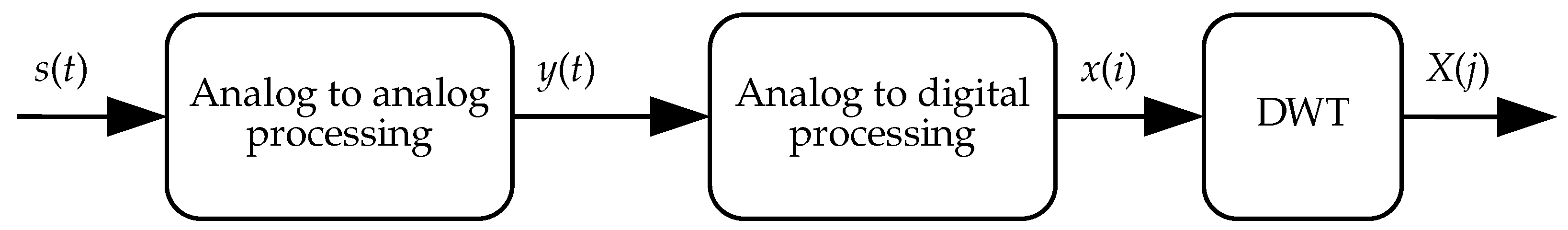
Considering the properties of the measurement chain that depend on the transmittance of fragments of this chain, it is worth analyzing these properties in the frequency domain. This approach enables a deterministic description of the influence of the transmittance on the input and processing of errors, while this description takes into account the spectrum of the processed measurement signal [18]. Let us assume that the analyzed measurement chain processes a physical quantity that changes over time, marked as . This quantity is converted by the analog part of this circuit into a voltage signal , which in the quantization process is converted into its discrete representation. Subsequent samples of this signal are marked with the symbol . The signal is sampled with the frequency , and N samples of this signal are taken in the measurement window, and then applied to the input of the stage computing the discrete wavelet transform algorithm. The algorithm discussed provides the output of the measuring chain which is a vector of M output quantities, marked as . A block diagram of the measuring chain is shown in Figure 1.
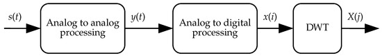
Figure 1.
Scheme of an exemplary measuring chain.
Further, the signal processed by the measurement chain is described as:
where is the pulsation of the i-th harmonic of this signal, is the amplitude and is the phase shift of the selected harmonic of this signal with pulsation . In the real case, the signal that is disturbed by the resultant error signal can be represented as:
where is the amplitude and is the phase shift in the selected harmonic of the error signal, and is the signal associated with a random error. It is assumed that, in Equations (19) and (21), the constant component of the described signals constitutes harmonics with index , where and . The properties of the signal in question must be determined at the stage of designing the measurement chain or identified in the case of an existing chain, which will be presented in an example later in this paper.
3.1. Analog Part of the Measurement Chain
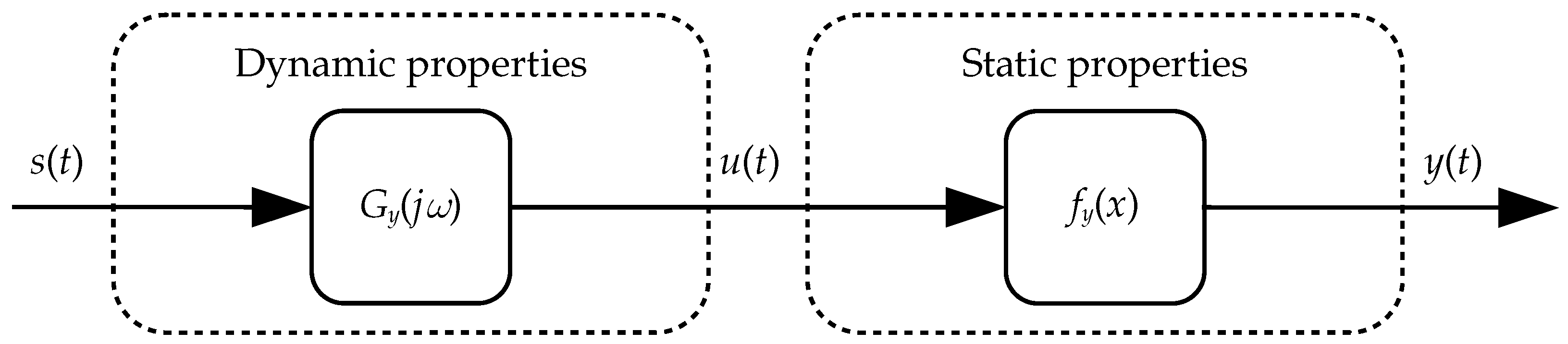
The analog part of the measurement circuit, which converts the signal into its voltage representation, marked as , can be described by a model using the transmittance and the processing function in accordance with the diagram shown in Figure 2. Based on the proposed scheme, the output quantity of the object can be described as:
where is the resultant error signal included in the output quantity which will be discussed in more detail later in this paper.
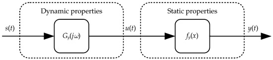
Figure 2.
Model of a fragment of the analog part of the measurement chain.
Knowing the transmittance makes it possible to determine the gain and the phase shift as a function of pulsation:
and, based on the gain , it is possible to determine the variation in the processed signals at the output of the fragment representing the dynamic properties of the object in accordance with the relationship [19]:
where is the variance in the signal as a function of pulsation. The presented relationship can be used to determine the variance in both random and deterministic signals. According to the diagram presented in Figure 2, the quantity can be described as:
where subsequent harmonics of this quantity are described by the following equations:
where is the ideal and the real gain value, while is the ideal and the real phase shift. Analyzing Equation (31), two components of this equation can be distinguished. The first component corresponds to the propagation of the ideal signal through the analyzed fragment and, due to the imperfection of this object (i.e., the discrepancy between the ideal and the real transmittance of the object), is responsible for its own signal error being introduced into the signal . The second component is related to the propagation of the error signal contained in the processed quantity through the analyzed part of the object.
In the case of static error signals, which are part of the resultant error signal , whose subsequent realization values do not change during a single measurement window, the following relationships can be written:
where is the own static error signal and is the static error signal propagated by the part of the object related to its dynamic properties. The dynamic error self signal introduced into the signal can be expressed as the sum of the subsequent harmonics of this signal as
The dynamic error signals contained in the input signal are propagated to the output of the analyzed part of the object in such a way that they are amplified and shifted, which is described by the following equation:
where is the dynamic error signal propagated from the input to the output of the fragment representing the dynamic properties of the analyzed fragment of the object. For propagated random error signals , it is impossible to determine the deterministic form of these signals, and therefore only their variances should be determined based on Equation (27). In order to determine the average value of the variance in the signals of propagated random errors in the pulsation interval , it is possible to use the following equation [18]:
however, this activity should be carried out only at the last stage of the analysis, where subsequent fragments of the measurement chain will not affect the spectrum of the processed random error signals. The error signals contained in the quantity described so far constitute the resultant error signal associated with this quantity, with
The symbol denotes an additional component constituting a random error introduced by the object, the variance of which is marked with the symbol .
Next, the signal is processed according to the object processing function ; therefore
It should be noted that the real form of the discussed function may actually differ from the ideal form assumed by the designer of the measurement chain. In the real case we can write
where is a function that takes into account selected quantities disturbing the process of determining the value of quantity (e.g., environmental parameters). Based on Equation (39), one can distinguish the own error signal , which results directly from the imperfection of the object processing function, and the own error signal , which results from the participation of disturbing factors. These signals can be described as:
The error signal will be deterministic if the form of the function is known. Otherwise, it is possible to describe its parameters in a probabilistic category. The nature of the error signal will depend on the properties of the analyzed object. In the case of the influence of environmental parameters on the measurement process, it can be assumed that these values will be slowly changing, hence this signal will usually be included in the group of static error signals. The variance in the signal at the output of the fragment representing the static properties of the object can, in general, be described by the equation [19]:
where is the expected value of signal realization . If the processing function of the object is a linear equation in the form , this analysis is simplified. By denoting the slope coefficient of the presented equation with the symbol , which can be identified with the sensitivity of the analyzed object, Equation (42) takes the form [19]:
It is important that the shift parameter b has no effect on the variance in the object’s output signal. If the processing function described is additive (when occurs for any parameters a and b belonging to the domain of this function), it is possible to analyze each of the error signals included in the signal separately. In this case it may be written as:
If the actual form of the processing function is not known, the ideal form of this function should be used in the calculations. This operation will result in an incorrect estimation of the error signal parameters, but is not possible in any other way.
The presented relationships make it possible to determine the parameters of error signals at the output of the analyzed object, both when the object processes errors that already exist in the input signal and when it introduces its own errors resulting from the imperfections of its properties. It should be noted that direct knowledge of the transmittance of the object is not necessary to perform the analysis, it is enough to estimate the actual gain and phase shift related to the dynamic properties of the object as a function of pulsation.
3.2. Properties of the Analog-to-Digital Converter
The analog-to-digital converter (ADC) has a discrete set of possible output values, and therefore introduces an error related to quantization into the output signal (where , and ). This error can be described in the form [21]:
where q is the value of a single quantum and is the value of the ADC output for the input voltage value equal to x, expressed in the unit of the input quantity. It can be noticed that the realization values of the discussed error signal depend on the realization values of the ADC input quantities. According to the research results presented in [12,21,22,23], this correlation can be neglected. Therefore, we propose describing the signal associated with the i-th realization of the quantization error using an uncorrelated additive noise model with the same probability of obtaining each of the possible realization values in the interval:
therefore, the variance in this signal can be determined according to the relationship [13]:
Given the above assumptions, in the ideal case the output value of the ADC can be given by the equation:
where is the selected time at which the input signal was sampled. In the real case, the quantity can be described as:
The resulting error signal at the output of the ADC can therefore be described as:
where is the error signal related to the rounding operations introduced in accordance with Equation (45), the variances of which are described by Equation (47), while is an additional self-error signal. Moreover, for an ideal quantizer system . Therefore, the variance in the signals at the output of the A/D converter can be described by the equation:
where is the variance in the signal at the object input. These assumptions allow us to assume that the analyzed object has no influence on the form of processed error signals:
where is the error signal at the output of the ADC related to the error signal at its input. The validity of the adopted assumptions was demonstrated, among others, in [17,21].
In the case of a real ADC, it is necessary to determine the parameters of the self-error signal, and this error most often results from ADC integral nonlinearity, differential nonlinearity, gain error, zero error, the heterogeneity of the internal structure of the converter or the imperfection of the reference voltage source [24,25]. Additionally, parameters related to the sample-and-hold circuit (S/H) should be considered separately. In this case, the model proposed for the analog part of the measurement chain, the parameters of which will be appropriate for the S/H circuit, will be used.
3.3. Digital Part of the Measurement Chain
If the input values of the wavelet transformation algorithm are processed by an additional object implementing digital-to-digital (D/D) or simply purely digital processing, it is proposed to describe the properties of this object in the same way as for the analog part of the measurement chain. The transmittance of the object in the domain should be transformed by substituting , as described in [14]. The further part of the analysis is analogous to the described case of the analog part of the measurement chain, so it will not be considered further in this article.
4. Application of the Proposed Analysis Method
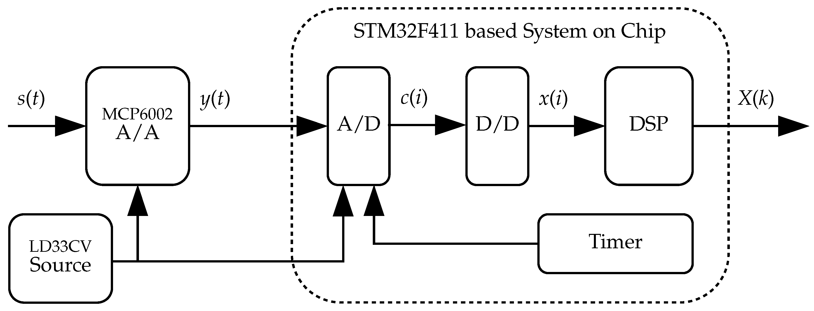
To verify the presented thesis, a prototype of a measuring circuit processing a time-varying voltage signal from the range was built. The first part of the measurement chain is an amplifier which adjusts the parameters of the processed signal to the operating range of the ADC. This amplifier has a transmittance of , which is responsible for introducing dynamic errors into the processed signal which can be described in a deterministic way. The output signal of the amplifier is processed by the ADC, whose successive output samples are processed by the discrete wavelet transform algorithm. A diagram of the measurement circuit is shown in Figure 3. The target gain of the analog part is V/V, and the phase shift should be zero. The processed signal is sampled with a constant frequency of kHz, and, on the basis of samples of the input value, samples of the output values of the measurement chain are determined. The additional D/D conversion element converts the original output signal of the ADC into output samples where , which in effect eliminates the static gain of the measuring amplifier. According to presented assumptions the quantity, which is a data source for the DWT algorithm, can be described as:
where static gain V/V and is described in next part of paper.

Figure 3.
Schematic representation of the prototype of the measuring chain, being the object of the experiment.
The exemplary measurement circuit was built on the basis of the STM32F411 microcontroller and the 12 bit built-in ADC [26]. The DWT algorithm was implemented using the DSP instruction and the “CMSIS DSP” library [27]. The amplifier was based on the MCP 6002 operational amplifier [28], operating in a non-inverting configuration with a gain of 3.29 V/V. The reference voltage source for the ADC, and, at the same time, the power source of the operational amplifier, was the LD33CV integrated circuit [29]. The reference voltage was additionally filtered to reduce noise.
4.1. Deterministic Errors Sources
The first step of analysis is to determine static and dynamic error signals parameters. In the case of constant environment parameters (temperature, pressure, humidity) it can be assumed that static errors do not exists in the presented system. In the case of any possible change in the described parameters it is necessary to describe how the analyses’ parameters impact the measurement chain. In the case of a dynamic error, the origin of this error will be the real transmittance of the measuring amplifier, which is different from the transmittance . Therefore, this transmittance must be determined or the parameters marked with Equations (25) and (26) should be determined by experiments. As the exact model of the operational amplifier used was unknown, an experiment was carried out in which a sinusoidal signal was applied to the input of the amplifier its gain and the phase shift was measured. The source of the signal was an RIGOL DG1011 arbitrary waveform generator [30], while the and signals’ parameters were measured with an RIGOL DS5062MA DSO [31] using mean value of 256 subsequent samples. For the experiment described here, the frequency of input signal was within range . The measurements enable the determination of the relationship between the gain and the phase shift introduced by the applied measuring amplifier as a function of pulsation.
As none of the typical filter models were applicable in the described situation, on the basis of the obtained values, approximations of the tested characteristics were carried out using polynomials, using the least squares method, whereby:
where is the gain, while is the phase shift in the selected harmonic of the processed signal. The relationships presented will enable the description of the waveform of the output signal of the measuring amplifier and, as a result, the determination of the waveform of the error signal introduced by this element.
Another dynamic error source is the S/H circuit at the input of the ADC. According to the manufacturer’s data, the S/H circuit can be described as a two-stage low-pass passive RC filter [25,26]. The first filter stage is formed by the internal impedance of the input voltage source and circuit capacitance. As the output impedance of the amplifier is relatively low, the influence of the first filter stage can be omitted [13,24,25]. The second filter is formed by the ON resistance of the internal S/H switch and a capacitance of typical values 5 k and 6 pF, respectively [25,26]. The resulting cutoff frequency of this filter is relatively high in comparison to the bandwidth of the amplifier so influence of the second filter can be neglected as well.
4.2. Random Errors Sources
In the case of random error signals, there are many more sources related to them and they occur in the whole measurement chain. It must be noticed that all phenomena for which a deterministic description is not possible must be considered as random error sources. These phenomena are, e.g., noise present in the input signal, the reference voltage and supply voltage, quantization errors, internal structure heterogeneity, integral errors and differential errors. As the analysis of all these phenomena separately is not possible without detailed knowledge of the parameters and the internal structure of the components used, we propose estimating the parameters of the resulting random error signal by performing the experiment described next.
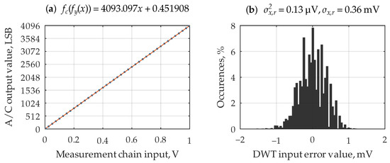
In the experiment, a nominally constant voltage was applied to the input of the measurement chain from a voltage source. Then, for the selected input voltage value, many implementation values of the quantity were taken. Based on the average obtained values of the realization of the quantity , it is possible to determine the static characteristics of the part of the measurement circuit which includes the amplifier and the measuring transducer, as well as to determine the inverse function for it, which will enable the reconstruction of the quantity in the form of the quantity . To allow this, it is necessary to repeat the experiment for subsequent input voltage values.
The described experiment was carried out in each k-th measurement series of 30,000 values for the realization of the quantity of the input voltage values in the range , where this value changed by mV for each measurement series. Based on values obtained for the realization of the quantity , the average value of these realizations was determined for the k-th measurement series. Then, on the basis of the obtained results, a linear approximation of the characteristics of the processing of the quantity to the quantity was performed:
where is the set voltage value for the analyzed series of measurements. Assuming that the sensitivity of quantity with respect to quantity is 1 V/V, the estimated average value of as a function of the value of can be described as:
The voltage source for the signal used in the experiment was the RIGOL DG1011 arbitrary waveform generator [30]. It was assumed that the errors introduced by the generator are negligible in relation to the errors arising in the analyzed section of the measurement chain.
It can be noticed that the static characteristic described by Equation (58) is a processing function for the part of the measurement chain that converts the quantity into the quantity . By determining the standard deviation of the differences between the measured realization values and the values determined in accordance with Equation (58), the standard uncertainty value related to the nonlinearity of the discussed characteristic is obtained. Additionally, on the basis of all the realization values of the quantity , it is possible to determine a histogram of the realization of the random error signal of this quantity, obtained under the experimental conditions.
Assuming that there were no non-random sources of error during the experiment (constant ambient conditions, constant input voltage for the analyzed series of measurements), the random error signal related to quantity can be described as:
while the random error signal of quantity can be described in the form:
Hence, based on the subsequent values of the error signal and Equations (57) and (58), the parameters of the error signal can be estimated. Figure 4a shows a graph of the characteristics given by Equation (57) obtained for the measurements, while Figure 4b shows a histogram of the error signal realization values calculated in accordance with Equation (59). Based on the indicated histogram, it is possible to estimate the variance in this signal equal to and the associated standard uncertainty mV. Based on the shape of the histogram, it can be concluded that the distribution of the error signal in question is a normal distribution with an expected value of zero.
4.3. Model Application for a Monoharmonic Input Signal
Analyzing Equations (34) and (35) in the case of the non-ideal dynamic properties of the measurement chain, it can be noticed that the parameters of the described signals will depend on the spectrum of the signal processed by the measurement chain. The first example of the application of the proposed model concerns a case in which this circuit processes a sinusoidal input signal with a given frequency , amplitude and direct-current (DC) component . This signal can be described by the equation:
whereas in the experiment it is assumed that . According to the assumptions that the environmental conditions do not change during subsequent measurement series and that the errors introduced by the arbitrary waveform generator used are negligibly small in relation to those introduced by the measurement chain, it can be assumed that the signal is not disturbed by any error signals, therefore .
Based on Equation (55), it can be noted that, in the frequency range , the value of the amplification introduced by the measuring amplifier is constant and is compensated by the static playback algorithm, in accordance with Equation (58). It can therefore be concluded that the only important parameter from the point of view of the error model will be the value of the phase shift introduced by the measuring amplifier, which is the cause of the dynamic self-error signal, depending on the pulsation of the input signal. The signal in question can be defined based on Equation (34):
where , and the value of is estimated according to polynomial (56). The form of the error signal described in Equation (62) consists of two factors with the same frequency, the resultant parameters of which can be be estimated in accordance with the content of equations from (12) to (18). By transforming the indicated equations and taking into account the components of Equation (62), the variance in the dynamic error signal can be determined in accordance with the relationship:
It can, therefore, be seen that the variance in the described signal depends on the signal frequency and its amplitude.
To summarize the considerations, the resultant error signal of the input quantity of the DWT algorithm in the discussed case will consist of the random error signal , the parameters of which were estimated previously, and the dynamic error signal , whose parameters are estimated according to Equation (63) for the given signal parameters . As the analyzed error signals are not correlated with each other, the variance of the resulting error signal can be estimated according to equation [13]:
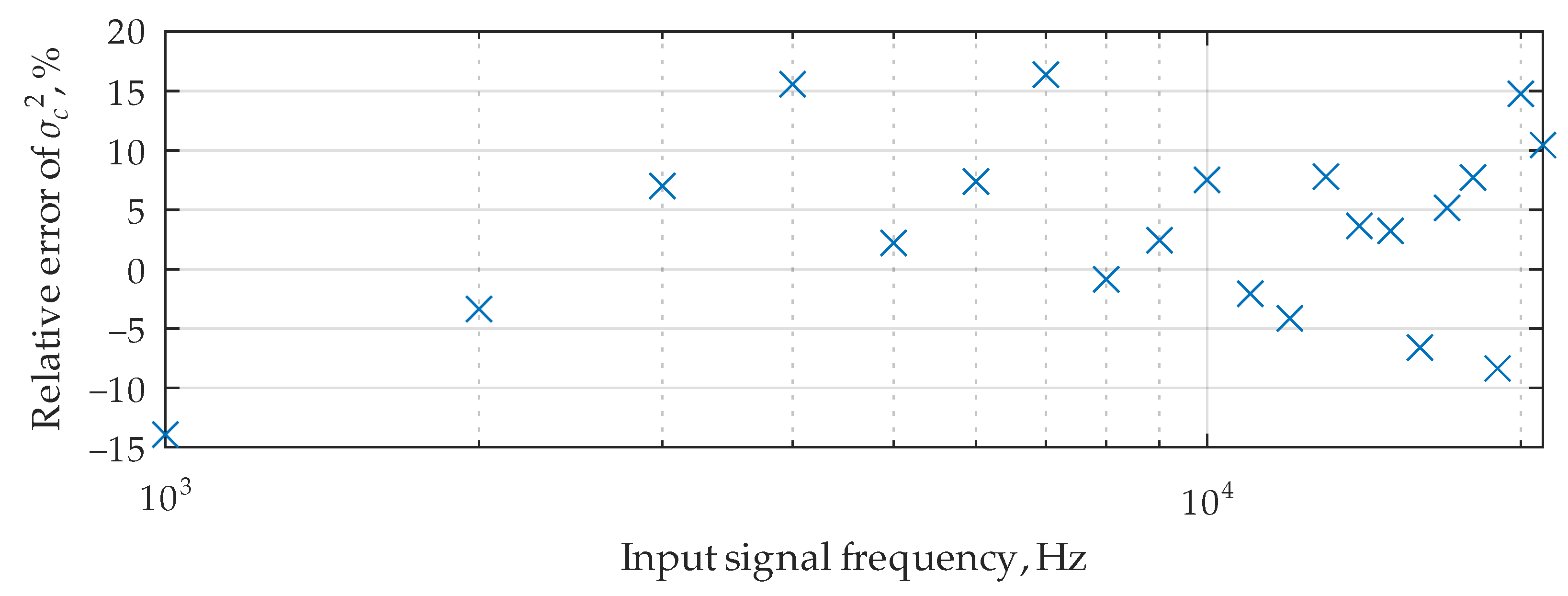
To verify the validity of the indicated relationships, a Monte-Carlo measurement experiment was carried out, in which 30,000 values of the signal realization were collected each time. During the experiment, the source of the signal was the RIGOL DG1011 arbitrary waveform generator [30], and the initial phase of this signal was randomized from the interval , and the generator’s synchronizing output was used to determine it. The frequency of the signal was in the range , while the parameters of this signal were constant and were V, V. Based on the obtained values of the realization of the quantity , in accordance with Equation (54), the values of the error signal were determined and the variances in this signal were calculated on their basis. The measured variance value was compared with the value determined according to Equation (64) and the relative error in estimating this value was calculated. The results for selected values of signal pulsation are summarized in Table 1, while calculated relative error values are also presented in Figure 5.

Table 1.
Experimentally determined and estimated values of the variance in the resultant error signal , where the symbol denotes the relative error of estimating the variance of the analyzed error signal (in the case of a monoharmonic input signal).
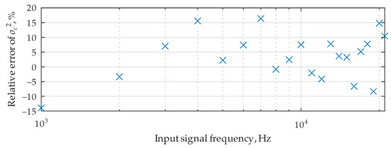
Figure 5.
Relative error of estimated values of the variance of the resultant error signal (in the case of a monoharmonic input signal).
4.4. Model Application for Poliharmonic Input Signal
In this section we assume that is a triangle signal. According to the assumptions, the processed signal can be described in the form:
where is a DC component of the signal, is the amplitude of the fundamental harmonic, is signal phase, is fundamental harmonic pulsation. In the experiment it was assumed that .
According to the previous assumptions, the parameters of the random error signal remain identical to those of the monoharmonic signal. However, a significant difference is in the parameters of the dynamic error signal , for which, according to Equation (34), the subsequent harmonics taken into account in Equation (65) should be analyzed. Therefore, for each harmonic of the error signal , its variance should be determined, similarly to the case of the monoharmonic signal. In the discussed case, for the i-th harmonic it occurs that:
wherein the amplitude for the i-th harmonic is determined according to the relationship:
The value of variance for the resultant error signal in the analyzed case can be determined according to the relationship:
however, we propose analyzing only those harmonics for which it occurs that for (all harmonic components for which the frequency is less or equal to the Nyquist frequency).
In order to verify the presented considerations, a measurement experiment using the Monte-Carlo method was carried out. In this case was a triangle signal with a given frequency in the range with parameters V, V and a random initial phase. For the selected signal frequency values, 30,000 samples of were taken in order to determine the value of the error signal based on Equation (54). Based on the obtained measurement results, the actual value of the variance in the analyzed error signal was determined and compared with the value estimated on the basis of Equation (68). The obtained results are summarized in Table 2. The source of the signal was an RIGOL DG1011 arbitrary waveform generator [30].
Table 2.
Experimentally determined and estimated values of the variance in the resultant error signal , where the symbol denotes the relative error of estimating the variance of the analyzed error signal (in the case of a polyharmonic input signal).
5. Reasons for Discrepancies in Results
Based on the results presented in Table 1 and Table 2, as well as on the basis of Figure 5, it can be noticed that the results obtained from the measurement experiment are not perfectly consistent with those obtained analytically. The main reason for the discussed discrepancies is the inaccurate determination of the parameters of the error model of the input quantities of the WT algorithm.
The measurement experiment carried out, the aim of which was to identify the static properties of the analyzed section of the measurement chain, assumed that the input values of the measurement chain were not encumbered with any errors. This simplification is inappropriate, and its elimination would require an identification of the properties of the arbitrary waveform generator used, which has not been carried out. Unfortunately, due to insufficient information being contained in the instrument documentation, the properties of the generator have to be determined experimentally.
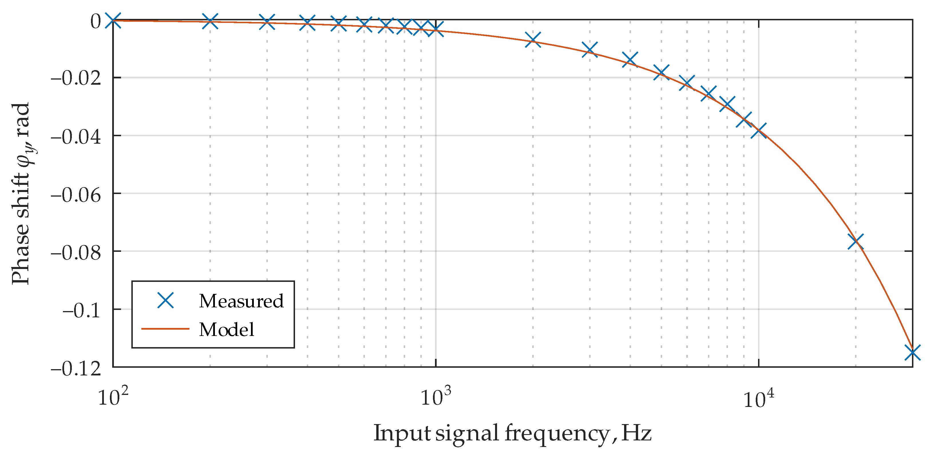
In the case of dynamic properties, a discrepancy between the actual and estimated value of the phase shift introduced by the analyzed measurement amplifier can be noticed. Figure 6 shows the measured and estimated values of the quantity in question based on Equation (56). In order to improve the obtained results, a higher order polynomial or a better model describing the properties of the measurement amplifier should be used.
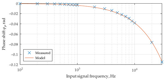
Figure 6.
Measured and estimated (according to the Equation (56)) values of phase shift introduced by amplifier.
The last simplification requiring discussion is the omission of the analysis of static error signals. As the experiment was performed under constant ambient conditions, the error signals in question did not occur. In reality, however, an appropriate measurement experiment should be carried out to identify them. For example, in the case of zero drift of the measurement amplifier and ADC converter, the influence of the ambient temperature on the introduced drift should be determined. Determining the parameters of the error signal in question enables its analysis in accordance with the method presented earlier in the work.
As the aim of the work was to indicate how to quantitatively describe the metrological properties of the measurement chain using the proposed error model, the work did not focus on a very precise determination of the parameters of the discussed model. In fact, the designer of the measurement chain should identify all error sources and indicate their parameters as precisely as possible. As there are works devoted to the analysis of subsequent fragments of the measurement path (e.g., in case of ADC works such as [22,24,25]), this work focused on an example with a minimum degree of complexity, while presenting results with an acceptable error.
6. Conclusions
Based on the results listed in Table 1 and Table 2 it can be seen that the estimated values of the variance in the resulting error signal of the input quantities of the DWT algorithm are close to those obtained by measurement. The proposed error model for the measurement chain allows to describe both deterministic and random error signals, and the parameters of these signals can be identified by measurement, as shown in the example presented. The example of a monoharmonic signal presented in this paper is the most simplified case, due to the presence of only one component of the dynamic error signal (in the discussed case, the dynamic error signal contains only one harmonic component). In the case of a polyharmonic signal, an example is presented in which a triangular signal was processed to indicate how to analyze many harmonics of the dynamic error signal and, therefore, many components of the resultant error signal of the output quantities. The presented analysis is performed identically for signals with any spectrum.
The application of the error model described in the article is simplified and does not take into account, among other things, error signals occurring in the input value of the measurement chain. The presented error model allows for a full analysis, while the adopted simplifications were justified by the need to present an example with a minimum degree of complexity. For the same reason, the analysis of static error signals was omitted. The mean of the absolute relative error values of the analyzed error signal was less than 10%, which means that a standard uncertainty value of relative error should be less than 5%. To improve accuracy of estimating discussed values a more precise measurement chain model parameter values must be obtained.
The example provided may constitute a set of guidelines for designers of measurement chains using WT algorithms on how to describe the metrological properties of the measurement chain so that a further analysis of the impact of these algorithms on the identified error signals is possible. The last step necessary to determine the uncertainty value of the output quantity of the measurement path presented in this work is to indicate how the analyzed WT algorithm affects the error signals identified in this article and present in the input quantities of this algorithm. The mentioned analysis was not presented in the current paper and is a separate issue, which will be discussed in subsequent works. Regardless of the number of error signals analyzed and the number of subsequent processing stages occurring in the measurement chain, the application of the presented error model is identical and its level of complexity does not change.
Author Contributions
Methodology, M.K.; Software, Ł.D.; Validation, M.K. and J.R.; Formal analysis, M.K.; Investigation, Ł.D.; Resources, Ł.D.; Data curation, Ł.D.; Writing—original draft, Ł.D.; Writing—review & editing, M.K. and J.R.; Visualization, Ł.D.; Supervision, J.R.; Project administration, M.K. All authors have read and agreed to the published version of the manuscript.
Funding
This research was partially funded by the Polish National Science Centre (NCN) grant number 2022/47/B/ST7/00047 and by Rector of Silesian University of Technology grant number 05/020/RGJ24/0084.
Institutional Review Board Statement
Not applicable.
Informed Consent Statement
Not applicable.
Data Availability Statement
The raw data supporting the conclusions of this article will be made available by the authors on request.
Conflicts of Interest
The authors declare no conflicts of interest.
Abbreviations
The following abbreviations are used in this manuscript:
| ADC | Analog-to-Digital Converter |
| CWT | Continuous wavelet transform |
| DC | Direct Current |
| D/D | Digital-to-Digital |
| DWT | Discrete wavelet transform |
| S/H | Sample-and-hold |
| WT | Wavelet transform |
References
- Unser, M.; Aldroubi, A. A review of wavelets in biomedical applications. Proc. IEEE 1996, 84, 626–638. [Google Scholar] [CrossRef]
- Ahmad, K. Wavelet Packets and Their Statistical Applications; Springer: Berlin/Heidelberg, Germany, 2018. [Google Scholar]
- Lord, G.J.; Pardo-Igúzquiza, E.; Smith, I.M. A Practical Guide to Wavelets for Metrology; National Physical Laboratory: London, UK, 2000. [Google Scholar]
- Akujuobi, C.M. Wavelets and Wavelet Transform Systems and Their Applications; Springer: Berlin/Heidelberg, Germany, 2022. [Google Scholar]
- Addison, P.S. The Illustrated Wavelet Transform Handbook: Introductory Theory and Applications in Science, Engineering, Medicine and Finance; CRC Press Inc.: Boca Raton, FL, USA, 2017. [Google Scholar]
- Wei, D. Coiflet-Type Wavelets: Theory, Design, and Applications; The University of Texas at Austin: Austin, TX, USA, 1998. [Google Scholar]
- Vonesch, C.; Blu, T.; Unser, M. Generalized Daubechies Wavelet Families. IEEE Trans. Signal Process. 2007, 55, 4415–4429. [Google Scholar] [CrossRef]
- An, P. Application of multi-wavelet seismic trace decomposition and reconstruction to seismic data interpretation and reservoir characterization. In SEG Technical Program Expanded Abstracts 2006; Society of Exploration Geophysicists: Houston, TX, USA, 2006; pp. 973–977. [Google Scholar]
- Hasan, O. Automatic detection of epileptic seizures in EEG using discrete wavelet transform and approximate entropy. Expert Syst. Appl. 2009, 36, 2027–2036. [Google Scholar]
- Yan, R.; Gao, R.X.; Chen, X. Wavelets for fault diagnosis of rotary machines: A review with applications. Signal Process. 2014, 96, 1–15. [Google Scholar] [CrossRef]
- Ruhm, K.H. Deterministic, Nondeterministic Signals; Institute for Dynamic Systems and Control: Zurich, Switzerland, 2008. [Google Scholar]
- Jakubiec, J. The error based model of a single measurement result in uncertainty calculation of the mean value of series. Probl. Prog. Metrol 2015, 20, 75–78. [Google Scholar]
- JCGM. Evaluation of Measurement Data—Guide to the Expression of Uncertainty in Measurement; JCGM: Paris, France, 2008; Available online: https://www.bipm.org/documents/20126/2071204/JCGM_100_2008_E.pdf/ (accessed on 16 April 2024).
- Oppenheim, A.V.; Buck, J.R.; Schafer, R.W. Discrete-Time Signal Processing; Prentice Hall: Hoboken, NJ, USA, 2001; Volume 2. [Google Scholar]
- Dieck, R.H. Measurement Uncertainty: Methods and Applications; ISA: Portland, OR, USA, 2007. [Google Scholar]
- Peretto, L.; Sasdelli, R.; Tinarelli, R. On uncertainty in wavelet-based signal analysis. IEEE Trans. Instrum. Meas. 2005, 54, 1593–1599. [Google Scholar] [CrossRef]
- Dróźdź, L.; Roj, J. Propagation of Random Errors by the Discrete Wavelet Transform Algorithm. Electronics 2021, 10, 764. [Google Scholar] [CrossRef]
- Proakis, J.G.; Manolakis, D.G. Digital Signal Processing: Principles, Algorithms and Applications; Prentice Hall: Hoboken, NJ, USA, 1996. [Google Scholar]
- Oppenheim, A.V.; Willsky, A.S.; Nawab, S.H. Signals & Systems, 2nd ed; Pearson: London, UK, 1996. [Google Scholar]
- Topór-Kaminski, T.; Jakubiec, J. Uncertainty modelling method of data series processing algorithms. In Proceedings of the IMEKO TC-4 Symposium on Development in Digital Measuring Instrumentation and 3rd Workshop on ADC Modelling and Testing, Naples, Italy, 17–18 September 1998; pp. 17–18. [Google Scholar]
- Gray, R.M.; Neuhoff, D.L. Quantization. IEEE Trans. Inf. Theory 1998, 44, 2325–2383. [Google Scholar] [CrossRef]
- Arpaia, P.; Baccigalupi, C.; Martino, M. Metrological characterization of high-performance delta-sigma ADCs: A case study of CERN DS-22. In Proceedings of the 2018 IEEE International Instrumentation and Measurement Technology Conference (I2MTC), Houston, TX, USA, 14–17 May 2018; pp. 1–6. [Google Scholar]
- Widrow, B. Statistical analysis of amplitude-quantized sampled-data systems. Trans. Am. Inst. Electr. Eng. Part II Appl. Ind. 1961, 79, 555–568. [Google Scholar] [CrossRef]
- Baker, B.C. Optimize Your SAR ADC Design; Texas Instruments Inc.: Dallas, TX, USA, 2019. [Google Scholar]
- STMicroelectronics. Application note AN1636; STMicroelectronics: Geneva, Switzerland, 2003. [Google Scholar]
- STMicroelectronics. Datasheet DS10314; STMicroelectronics: Geneva, Switzerland, 2017. [Google Scholar]
- ARM Limited. CMSIS-DSP; ARM Limited: Cambridge, UK, 2023. [Google Scholar]
- Microchip Technology Inc. Datasheet DS20001733L; Microchip Technology Inc.: Chandler, AZ, USA, 2019. [Google Scholar]
- STMicroelectronics. Datasheet DS2572; STMicroelectronics: Geneva, Switzerland, 2020. [Google Scholar]
- RIGOL Technologies Inc. User’s Guide DG1-070518; RIGOL Technologies Inc.: Beijing, China, 2007. [Google Scholar]
- Rigol Electronic Co., Ltd. User Manual DS5-040501; Rigol Electronic Co., Ltd.: Beijing, China, 2004. [Google Scholar]

Disclaimer/Publisher’s Note: The statements, opinions and data contained in all publications are solely those of the individual author(s) and contributor(s) and not of MDPI and/or the editor(s). MDPI and/or the editor(s) disclaim responsibility for any injury to people or property resulting from any ideas, methods, instructions or products referred to in the content. |
© 2024 by the authors. Licensee MDPI, Basel, Switzerland. This article is an open access article distributed under the terms and conditions of the Creative Commons Attribution (CC BY) license (https://creativecommons.org/licenses/by/4.0/).