


Offline Identification of a Laboratory Incubator


Abstract
:1. Introduction
2. Materials and Methods
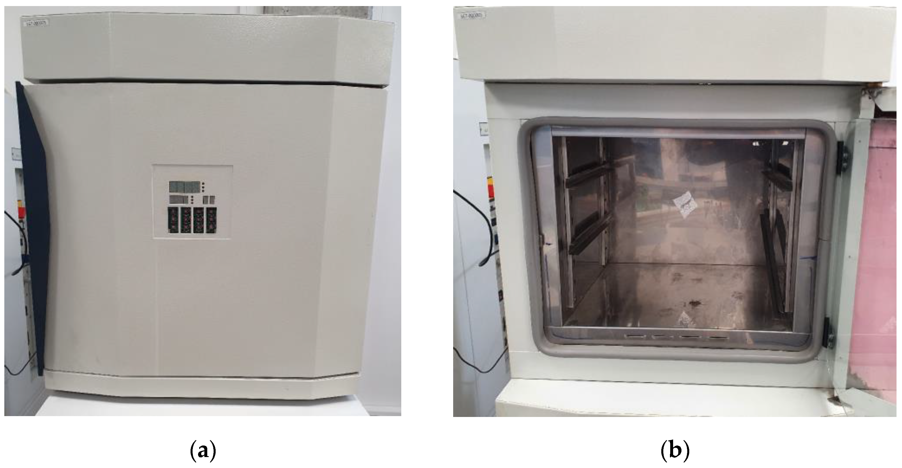
2.1. Laboratory Incubator
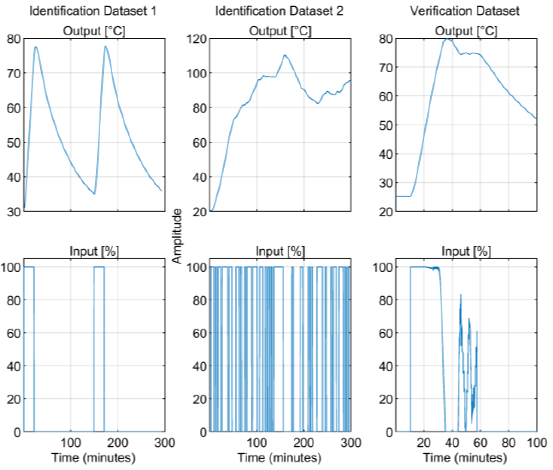
2.2. Data Collection
2.3. Data Preprocessing
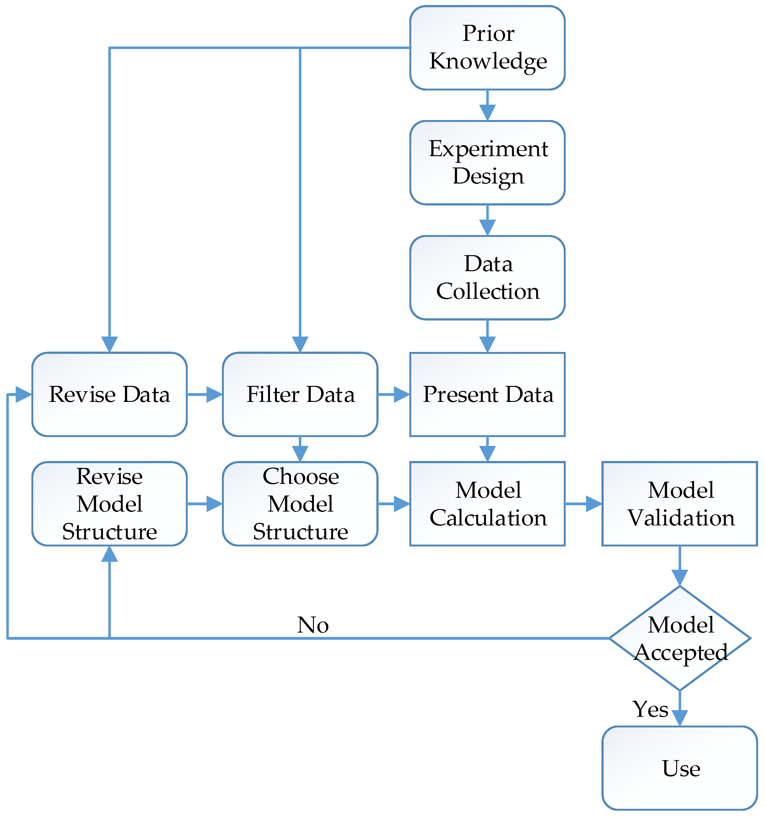
2.4. System Identification
2.5. Model Structures
2.5.1. Auto-Regressive Exogenous (ARX) Model
2.5.2. Auto Regressive Moving Average Exogenous (ARMAX) Model
2.5.3. Output Error (OE) Model
2.5.4. Box–Jenkins (BJ) Model
2.6. Estimating the Parameter Vector ()
2.7. Performance Evaluation
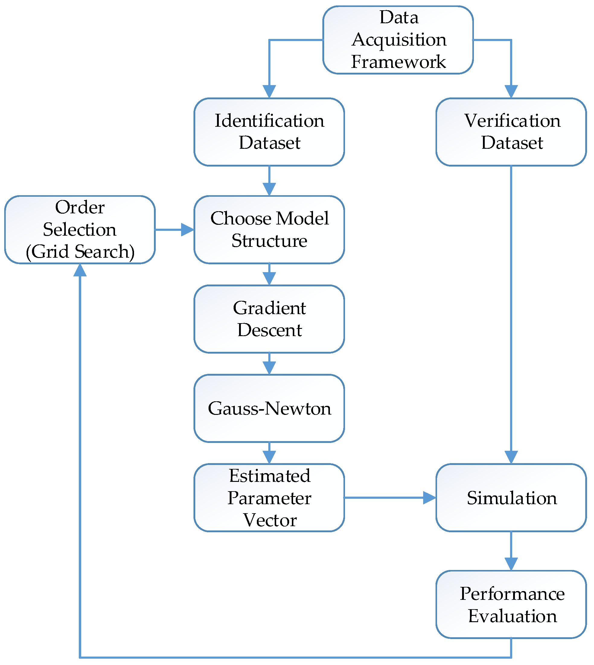
2.8. System Overview for Estimating the Parameter Vector ()
3. Experiments
3.1. Experiment Setup
3.2. Experimental Results
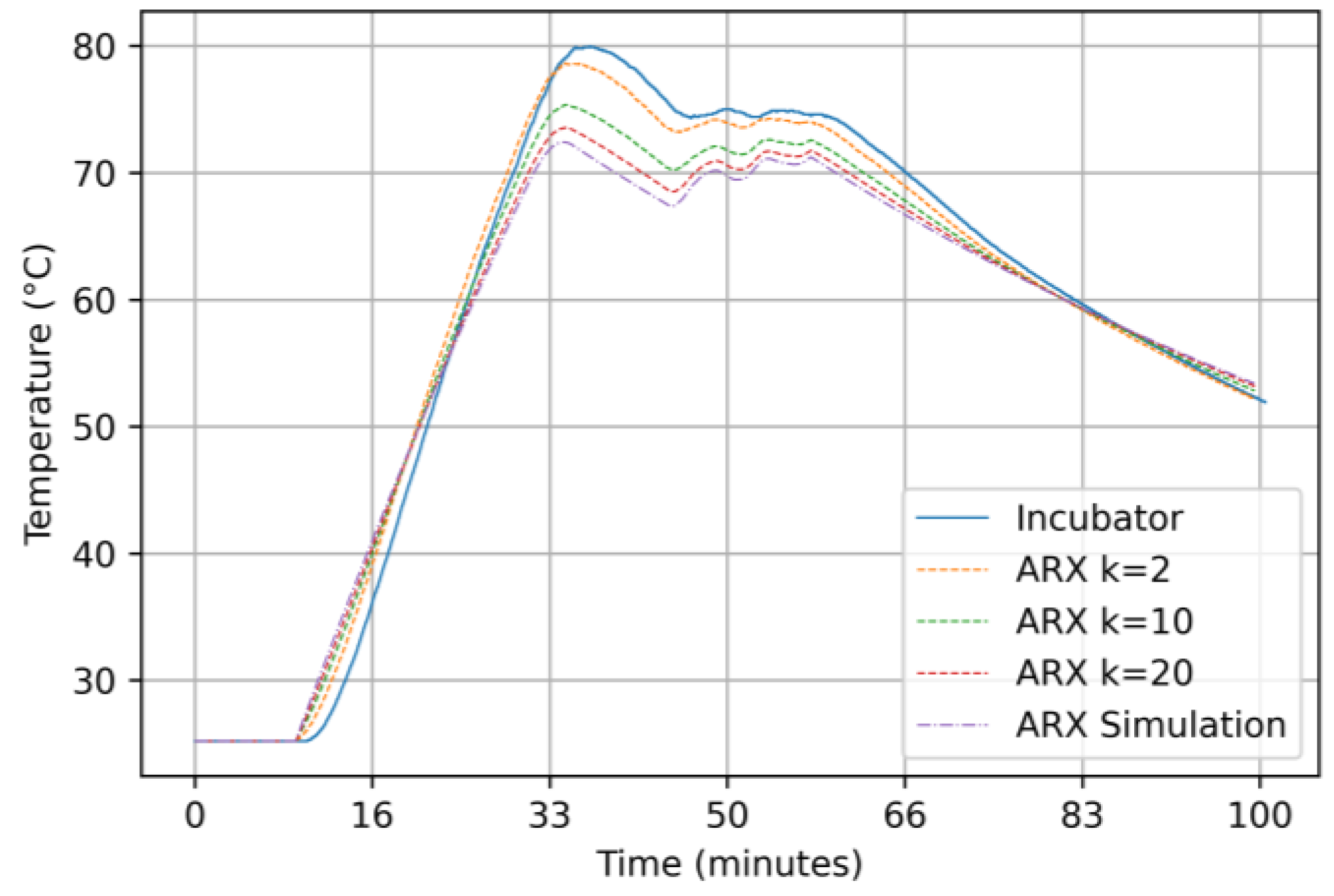
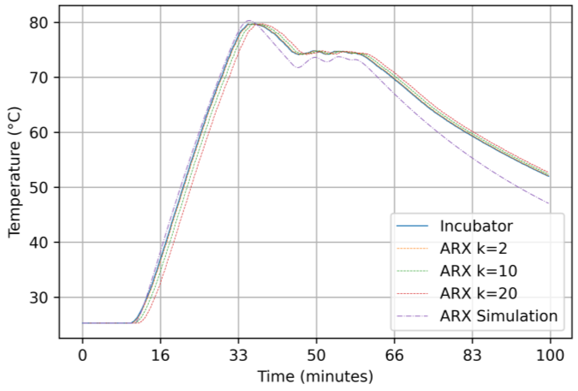
3.2.1. Results for the ARX Model
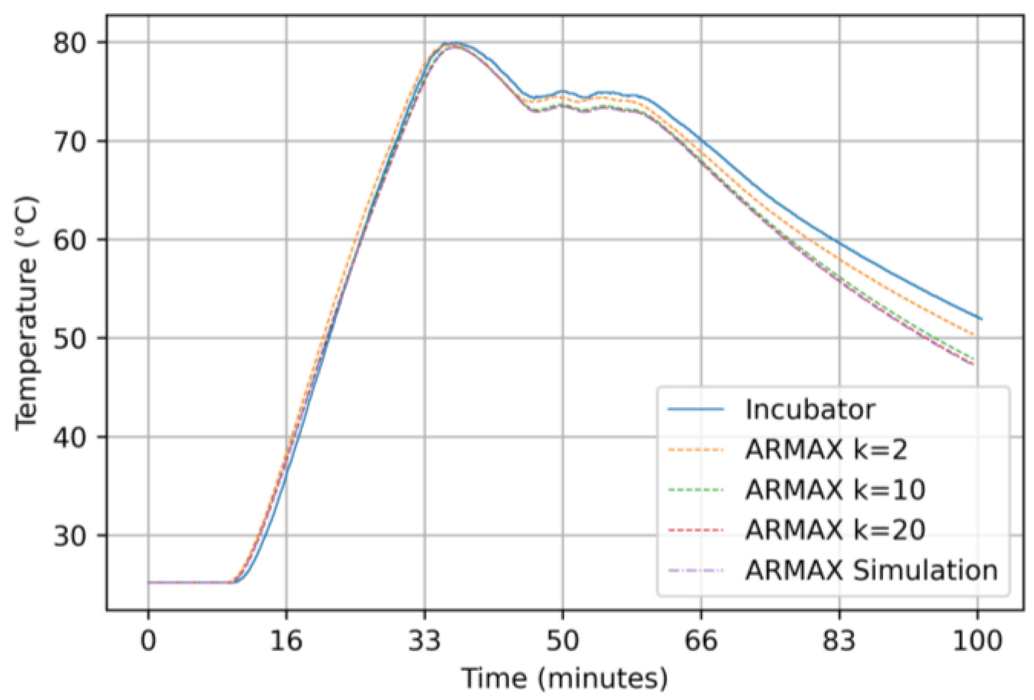
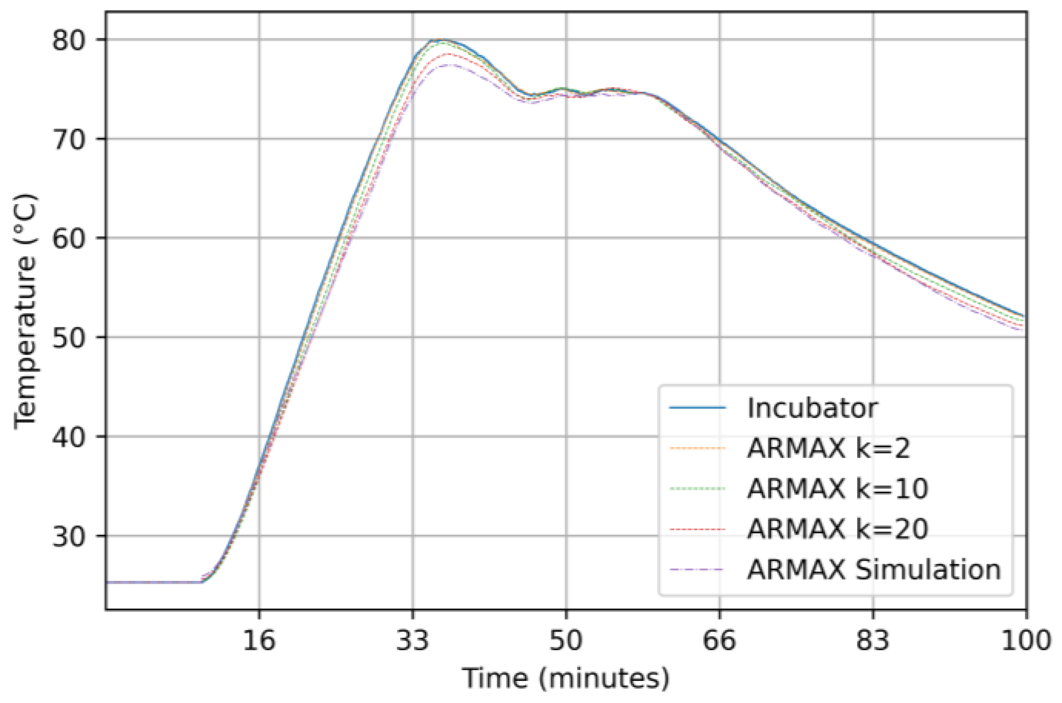
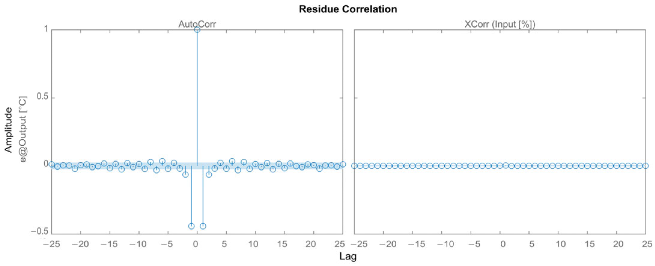
3.2.2. Results for the ARMAX Model
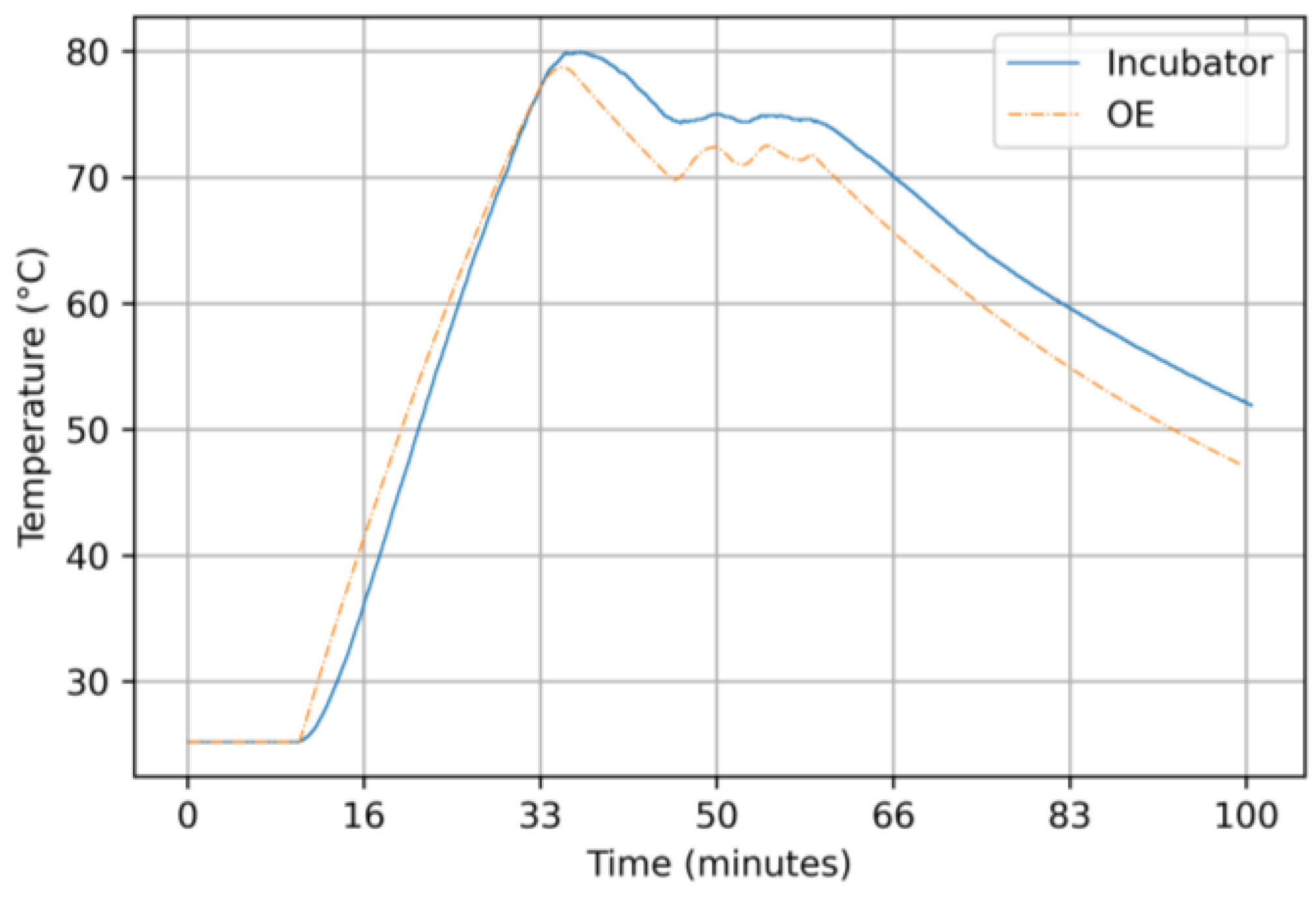
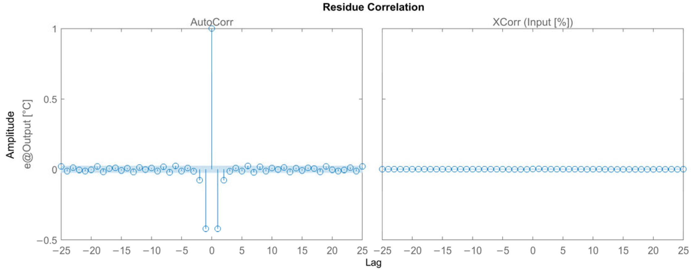
3.2.3. Results for the Output-Error Model
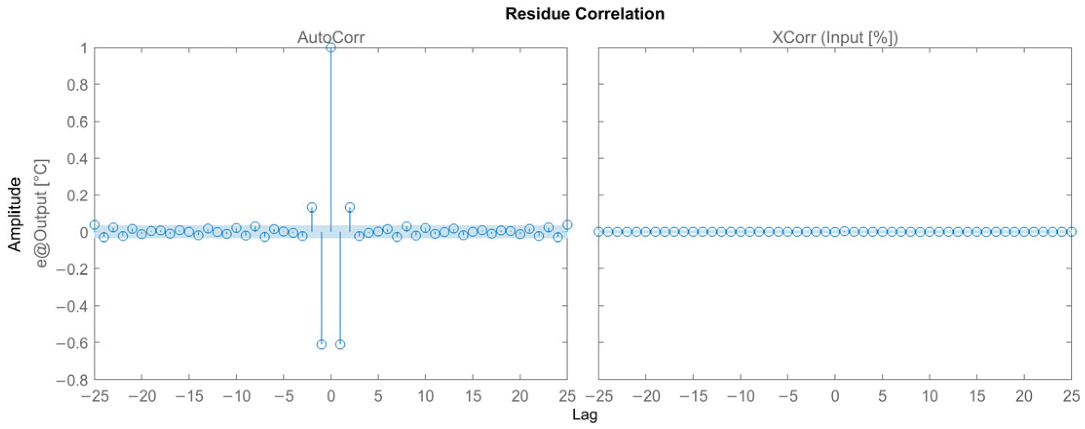
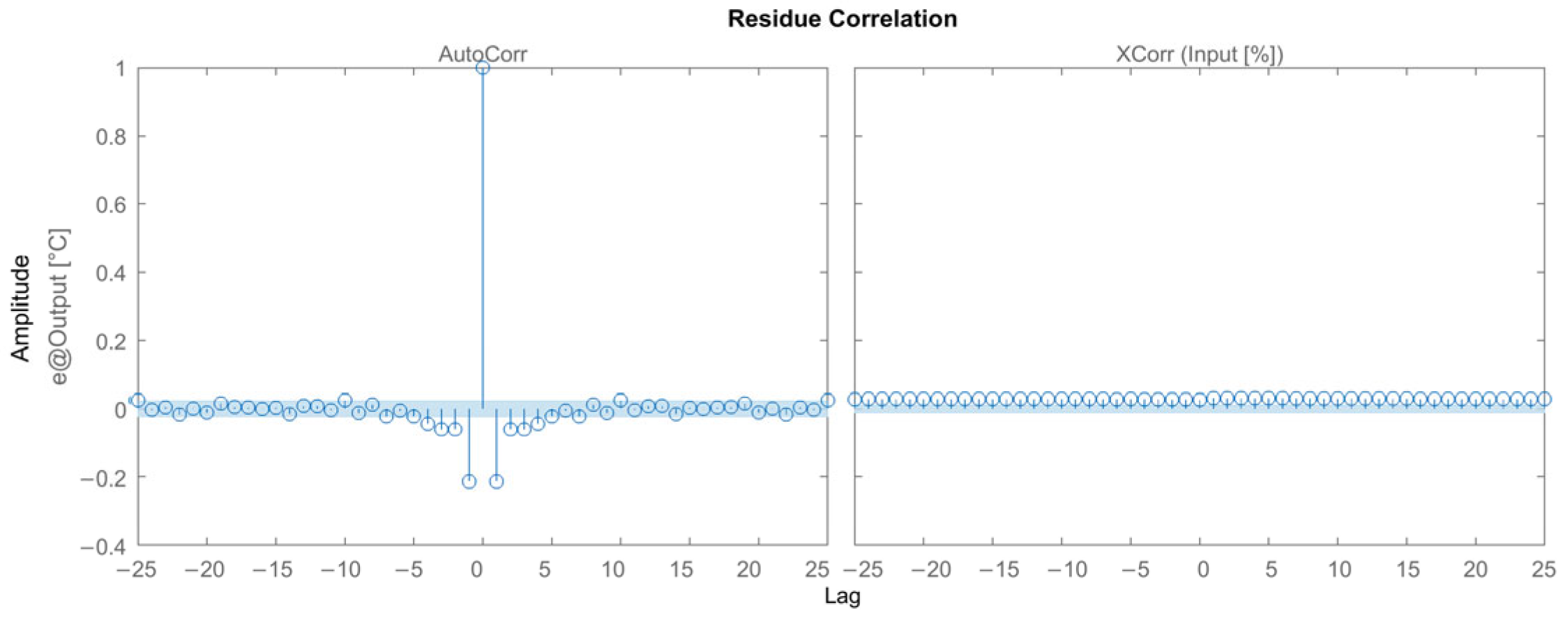
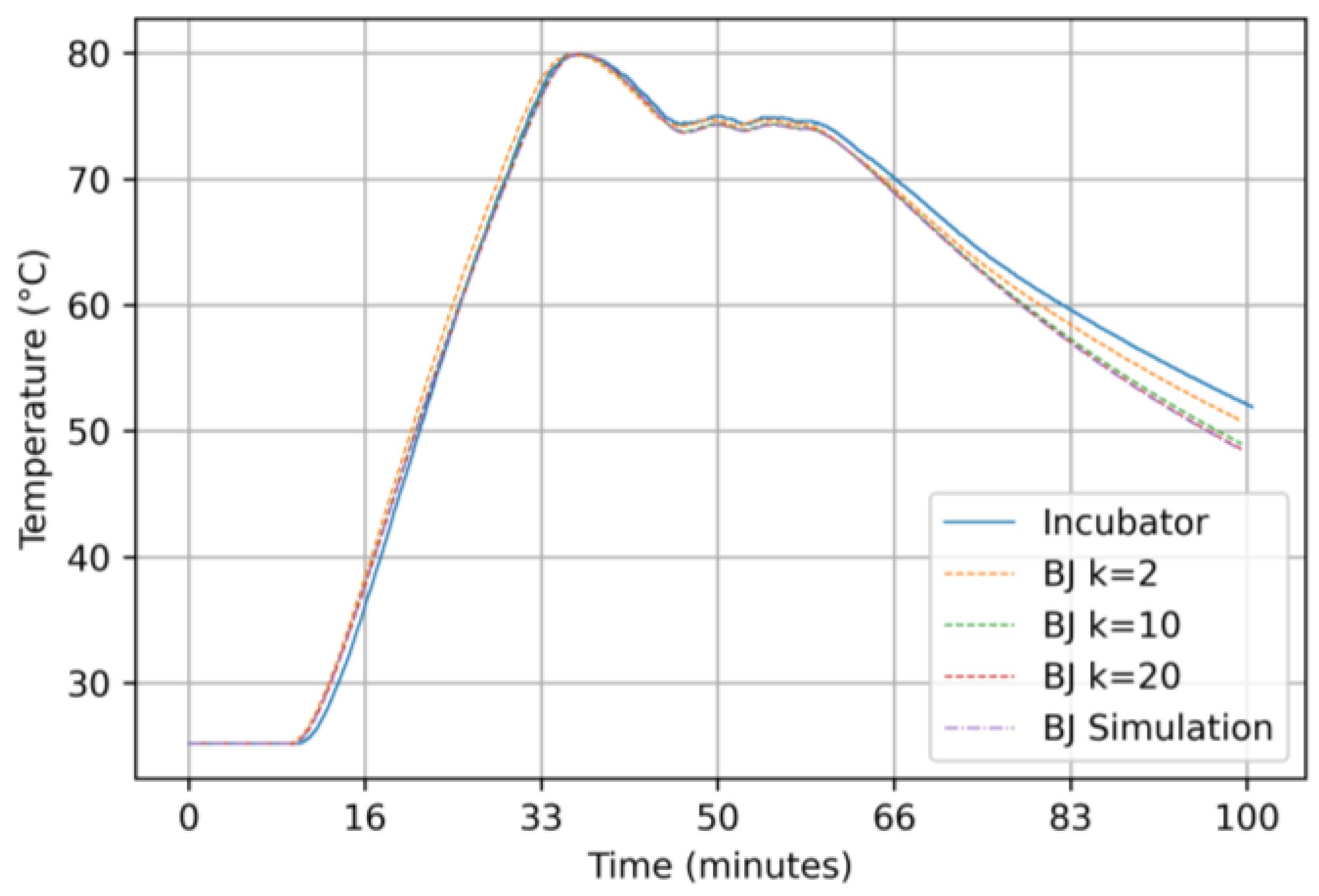
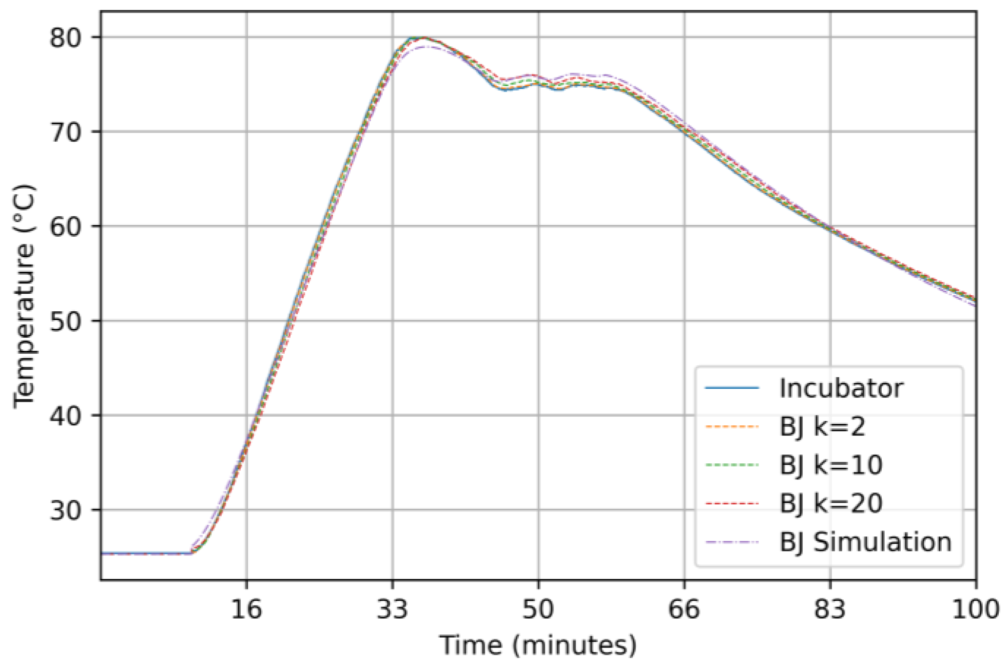
3.2.4. Results for the Box–Jenkins Model
4. Discussions
5. Conclusions
Author Contributions
Funding
Institutional Review Board Statement
Informed Consent Statement
Data Availability Statement
Acknowledgments
Conflicts of Interest
References
- Cappuccino, J.G.; Welsh, C.T. Microbiology: A Laboratory Manual; Pearson Education: London, UK, 2016; ISBN 9780134298597. [Google Scholar]
- Miller, A.K.; Ghionea, S.; Vongsouvath, M.; Davong, V.; Mayxay, M.; Somoskovi, A.; Newton, P.N.; Bell, D.; Friend, M. A Robust Incubator to Improve Access to Microbiological Culture in Low Resource Environments. J. Med. Devices Trans. ASME 2019, 13, 011007. [Google Scholar] [CrossRef] [PubMed]
- Pramuditha, K.A.S.; Hapuarachchi, H.P.; Nanayakkara, N.N.; Senanayaka, P.R.; De Silva, A.C. Drawbacks of Current IVF Incubators and Novel Minimal Embryo Stress Incubator Design. In Proceedings of the 2015 IEEE 10th International Conference on Industrial and Information Systems (ICIIS), Peradeniya, Sri Lanka, 18–20 December 2015; pp. 100–105. [Google Scholar] [CrossRef]
- Abbas, A.K.; Leonhardt, S. System Identification of Neonatal Incubator Based on Adaptive ARMAX Technique. In 4th European Conference of the International Federation for Medical and Biological Engineering; Springer: Berlin/Heidelberg, Germany, 2009; Volume 22, pp. 2515–2519. [Google Scholar] [CrossRef]
- Ljung, L. Perspectives on System Identification. IFAC Proc. Vol. 2008, 41, 7172–7184. [Google Scholar] [CrossRef]
- Kaya, O.; Abedinifar, M.; Feldhaus, D.; Diaz, F.; Ertuğrul, Ş.; Friedrich, B. System Identification and Artificial Intelligent (AI) Modelling of the Molten Salt Electrolysis Process for Prediction of the Anode Effect. Comput. Mater. Sci. 2023, 230, 112527. [Google Scholar] [CrossRef]
- Shen, H.; Xu, M.; Guez, A.; Li, A.; Ran, F. An Accurate Sleep Stages Classification Method Based on State Space Model. IEEE Access 2019, 7, 125268–125279. [Google Scholar] [CrossRef]
- Beintema, G.I.; Schoukens, M.; Tóth, R. Deep Subspace Encoders for Nonlinear System Identification. Automatica 2023, 156, 111210. [Google Scholar] [CrossRef]
- Gedon, D.; Wahlström, N.; Schön, T.B.; Ljung, L. Deep State Space Models for Nonlinear System Identification. IFAC-PapersOnLine 2021, 54, 481–486. [Google Scholar] [CrossRef]
- Oymak, S.; Ozay, N. Non-Asymptotic Identification of LTI Systems from a Single Trajectory. In Proceedings of the 2019 American Control Conference (ACC), Philadelphia, PA, USA, 10–12 July 2019; pp. 5655–5661. [Google Scholar] [CrossRef]
- Bagherian, D.; Gornet, J.; Bernstein, J.; Ni, Y.L.; Yue, Y.; Meister, M. Fine-Grained System Identification of Nonlinear Neural Circuits. In Proceedings of the 27th ACM SIGKDD Conference on Knowledge Discovery & Data Mining, Singapore, 14–18 August 2021; pp. 14–24. [Google Scholar] [CrossRef]
- Moradimaryamnegari, H.; Frego, M.; Peer, A. Model Predictive Control-Based Reinforcement Learning Using Expected Sarsa. IEEE Access 2022, 10, 81177–81191. [Google Scholar] [CrossRef]
- Armenise, G.; Vaccari, M.; Di Capaci, R.B.; Pannocchia, G. An Open-Source System Identification Package for Multivariable Processes. In Proceedings of the 2018 UKACC 12th International Conference on Control (CONTROL), Sheffield, UK, 5–7 September 2018; pp. 152–157. [Google Scholar] [CrossRef]
- Pillonetto, G.; Ljung, L. Full Bayesian Identification of Linear Dynamic Systems Using Stable Kernels. Proc. Natl. Acad. Sci. USA 2023, 120, e2218197120. [Google Scholar] [CrossRef] [PubMed]
- Fotouhi, A.; Auger, D.J.; Propp, K.; Longo, S. Electric Vehicle Battery Parameter Identification and SOC Observability Analysis: NiMH and Li-S Case Studies. IET Power Electron. 2017, 10, 1289–1297. [Google Scholar] [CrossRef]
- Gupta, S.; Gupta, R.; Padhee, S. Stability and Weighted Sensitivity Analysis of Robust Controller for Heat Exchanger. Control Theory Technol. 2020, 18, 56–71. [Google Scholar] [CrossRef]
- Fatima, S.K.; Abbas, S.M.; Mir, I.; Gul, F.; Mir, S.; Saeed, N.; Alotaibi, A.; Althobaiti, T.; Abualigah, L. Data Driven Model Estimation for Aerial Vehicles: A Perspective Analysis. Processes 2022, 10, 1236. [Google Scholar] [CrossRef]
- Bnhamdoon, O.A.A.; Mohamad Hanif, N.H.H.; Akmeliawati, R. Identification of a Quadcopter Autopilot System via Box–Jenkins Structure. Int. J. Dyn. Control 2020, 8, 835–850. [Google Scholar] [CrossRef]
- Paschke, F.; Zaiczek, T.; Robenack, K. Identification of Room Temperature Models Using K-Step PEM for Hammerstein Systems. In Proceedings of the 2019 23rd International Conference on System Theory, Control and Computing (ICSTCC), Sinaia, Romania, 9–11 October 2019; pp. 320–325. [Google Scholar] [CrossRef]
- DIN EN 60751; Industrial Platinum Resistance Thermometers and Platinum Temperature Sensors (IEC 60751:2022). International Electrotechnical Commission: Geneva, Switzerland, 2022.
- Ljung, L. System Identification: Theory for the User; Prentice Hall: Saddle River, NJ, USA, 1999; p. 609. [Google Scholar]
- Pillonetto, G.; Dinuzzo, F.; Chen, T.; De Nicolao, G.; Ljung, L. Kernel Methods in System Identification, Machine Learning and Function Estimation: A Survey. Automatica 2014, 50, 657–682. [Google Scholar] [CrossRef]
- Söderström, T.; Stoica, P. System Identification; Prentice-Hall International: Saddle River, NJ, USA, 1989. [Google Scholar]
- Verhaegen, M.; Verdult, V. Filtering and System Identification: A Least Squares Approach; Cambridge University Press: Cambridge, UK, 2007; pp. 1–405. ISBN 978-0521875127. [Google Scholar]
- Mustafaraj, G.; Chen, J.; Lowry, G. Development of Room Temperature and Relative Humidity Linear Parametric Models for an Open Office Using BMS Data. Energy Build. 2010, 42, 348–356. [Google Scholar] [CrossRef]


| Validation Criteria | G | MSE | MAE | |||
|---|---|---|---|---|---|---|
| Step | PRBS | Step | PRBS | Step | PRBS | |
| Prediction k: 2 | 95.6526 | 98.7377 | 5.47874 × 10⁻⁵ | 5.0382 × 10⁻⁶ | 0.00494216 | 0.0016 |
| Prediction k: 10 | 86.1103 | 94.1006 | 0.00055925 | 0.00011005 | 0.0175226 | 0.0074 |
| Prediction k: 20 | 80.7099 | 88.3159 | 0.00107867 | 0.00043167 | 0.0244397 | 0.0145 |
| Simulation | 77.2656 | 85.1858 | 0.00149826 | 0.00069394 | 0.0289541 | 0.0211 |
| Validation Criteria | G | MSE | MAE | |||
|---|---|---|---|---|---|---|
| Step | PRBS | Step | PRBS | Step | PRBS | |
| Prediction k: 2 | 94.9755 | 98.5564 | 7.3182 × 10⁻⁵ | 6.638 × 10⁻⁶ | 0.00645041 | 0.0020 |
| Prediction k: 10 | 87.8214 | 95.2388 | 0.000429946 | 7.2225 × 10⁻⁵ | 0.0167575 | 0.0065 |
| Prediction k: 20 | 86.247 | 92.2919 | 0.000548299 | 0.00018899 | 0.0189746 | 0.0105 |
| Simulation | 86.1957 | 90.5396 | 0.000552393 | 0.00028334 | 0.0191662 | 0.0128 |
| Validation Criteria | G | MSE | MAE | |||
|---|---|---|---|---|---|---|
| Step | PRBS | Step | PRBS | Step | PRBS | |
| Simulation | 83.0517 | 84.0369 | 0.000856901 | 0.00080505 | 0.0240122 | 0.0235 |
| Validation Criteria | G | MSE | MAE | |||
|---|---|---|---|---|---|---|
| Step | PRBS | Step | PRBS | Step | PRBS | |
| Prediction k: 2 | 96.2799 | 99.4335 | 4.01182 × 10⁻⁵ | 9.1998 × 10⁻⁷ | 0.0041233 | 0.0007 |
| Prediction k: 10 | 91.4721 | 98.1200 | 0.000210816 | 1.0131 × 10⁻⁵ | 0.0108614 | 0.0021 |
| Prediction k: 20 | 90.4577 | 96.4682 | 0.000263956 | 3.5756 × 10⁻⁵ | 0.0124288 | 0.0040 |
| Simulation | 90.3288 | 95.0771 | 0.000271132 | 7.0355 × 10⁻⁵ | 0.0123917 | 0.0074 |
| Validation Criteria | G | MSE | MAE | |||
|---|---|---|---|---|---|---|
| Step | PRBS | Step | PRBS | Step | PRBS | |
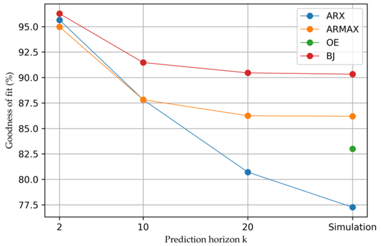
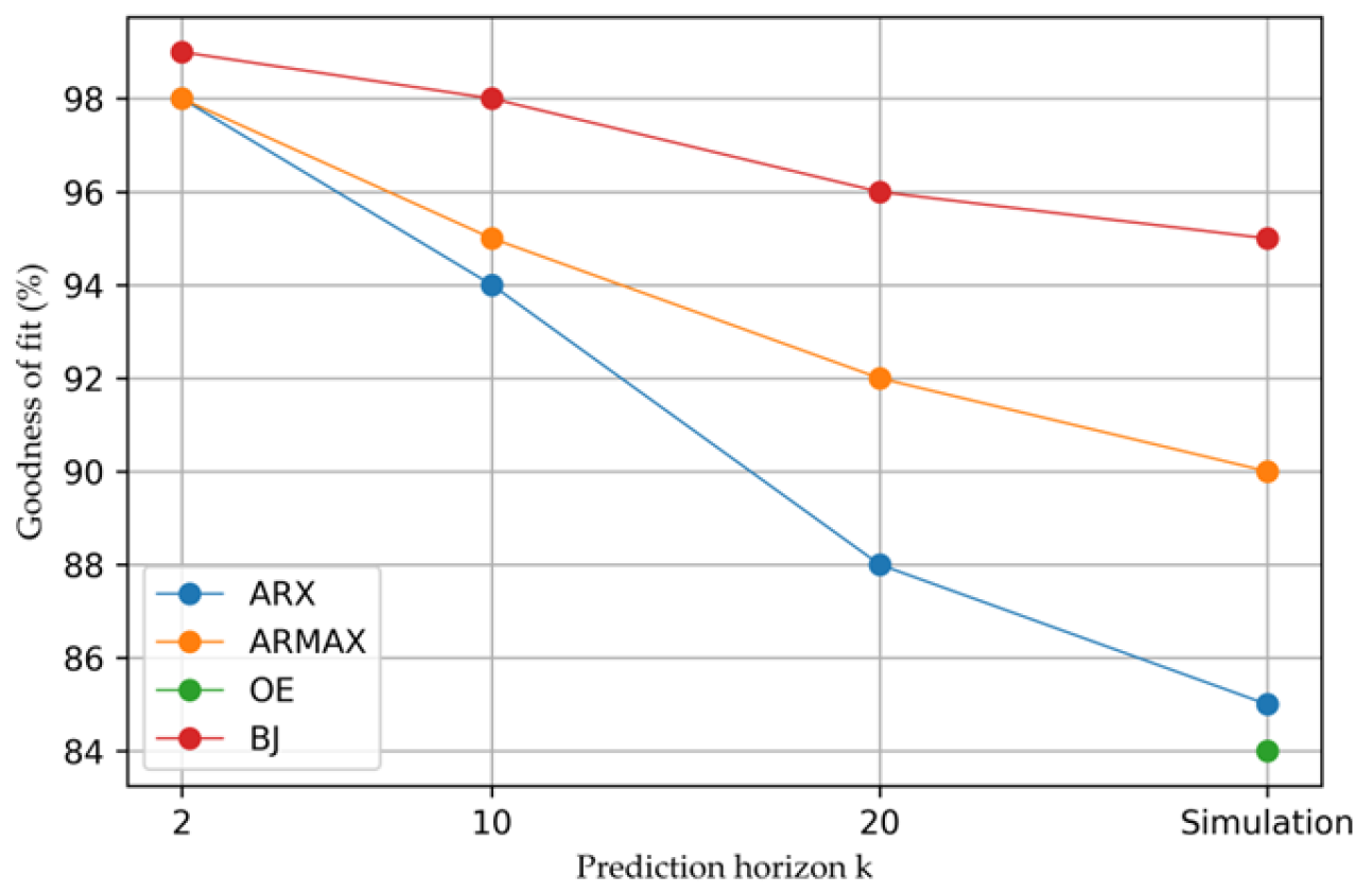
| ARX [2 2] | ||||||
| Prediction k: 2 | 95.6526 | 98.7377 | 5.47874 × 10⁻⁵ | 5.0382 × 10⁻⁶ | 0.00494216 | 0.0016 |
| Prediction k: 10 | 86.1103 | 94.1006 | 0.00055925 | 0.00011005 | 0.0175226 | 0.0074 |
| Prediction k: 20 | 80.7099 | 88.3159 | 0.00107867 | 0.00043167 | 0.0244397 | 0.0145 |
| Simulation | 77.2656 | 85.1858 | 0.00149826 | 0.00069394 | 0.0289541 | 0.0211 |
| ARMAX [2 2 2] | ||||||
| Prediction k: 2 | 94.9755 | 98.5564 | 7.3182 × 10⁻⁵ | 6.638 × 10⁻⁶ | 0.00645041 | 0.0020 |
| Prediction k: 10 | 87.8214 | 95.2388 | 0.000429946 | 7.2225 × 10⁻⁵ | 0.0167575 | 0.0065 |
| Prediction k: 20 | 86.247 | 92.2919 | 0.000548299 | 0.00018899 | 0.0189746 | 0.0105 |
| Simulation | 86.1957 | 90.5396 | 0.000552393 | 0.00028334 | 0.0191662 | 0.0128 |
| OE [2 2] | ||||||
| Simulation | 83.0517 | 84.0369 | 0.000856901 | 0.00080505 | 0.0240122 | 0.0235 |
| BJ [2 2 2 2] | ||||||
| Prediction k: 2 | 96.2799 * | 99.4335 | 4.01182 × 10⁻⁵ | 9.1998 × 10⁻⁷ | 0.0041233 | 0.0007 |
| Prediction k: 10 | 91.4721 | 98.1200 | 0.000210816 | 1.0131 × 10⁻⁵ | 0.0108614 | 0.0021 |
| Prediction k: 20 | 90.4577 | 96.4682 | 0.000263956 | 3.5756 × 10⁻⁵ | 0.0124288 | 0.0040 |
| Simulation | 90.3288 | 95.0771 | 0.000271132 | 7.0355 × 10⁻⁵ | 0.0123917 | 0.0074 |
Disclaimer/Publisher’s Note: The statements, opinions and data contained in all publications are solely those of the individual author(s) and contributor(s) and not of MDPI and/or the editor(s). MDPI and/or the editor(s) disclaim responsibility for any injury to people or property resulting from any ideas, methods, instructions or products referred to in the content. |
© 2024 by the authors. Licensee MDPI, Basel, Switzerland. This article is an open access article distributed under the terms and conditions of the Creative Commons Attribution (CC BY) license (https://creativecommons.org/licenses/by/4.0/).
Share and Cite
Mantar, S.; Yılmaz, E. Offline Identification of a Laboratory Incubator. Appl. Sci. 2024, 14, 3466. https://doi.org/10.3390/app14083466
Mantar S, Yılmaz E. Offline Identification of a Laboratory Incubator. Applied Sciences. 2024; 14(8):3466. https://doi.org/10.3390/app14083466
Chicago/Turabian StyleMantar, Süleyman, and Ersen Yılmaz. 2024. "Offline Identification of a Laboratory Incubator" Applied Sciences 14, no. 8: 3466. https://doi.org/10.3390/app14083466
APA StyleMantar, S., & Yılmaz, E. (2024). Offline Identification of a Laboratory Incubator. Applied Sciences, 14(8), 3466. https://doi.org/10.3390/app14083466