Article

High-Impedance Fault Detection in DC Microgrid Lines Using Open-Set Recognition

Faculty of Electrical Engineering and Computing, University of Zagreb, 10000 Zagreb, Croatia
*
Author to whom correspondence should be addressed.
Appl. Sci. 2025, 15(1), 193; https://doi.org/10.3390/app15010193
Submission received: 16 November 2024 / Revised: 20 December 2024 / Accepted: 27 December 2024 / Published: 29 December 2024

Abstract

:
Detection of high-impedance faults in direct current microgrid lines presents a challenge for most conventional protection schemes because the magnitude of the fault current is similar to other transients that occur during normal operation. However, the waveform of high-impedance faults differs from that of other transients as it is characterized by a repetitive and nonlinear pattern caused by current reignition. Various methods have been proposed to exploit fault response waveforms for detecting high-impedance faults, including those based on deep discriminative intelligent classification. Different from previous works that focus on closed-set classification, this study frames fault detection as an open-set recognition problem, employing a neural network as the classifier. The resulting approach enables the detection of high-impedance faults as outliers from the normal operating states of microgrid lines with passive constant impedance loads and requires only the Fourier transform of the current signal as input to the neural network. Remarkably, the proposed solution eliminates the need for hard-to-model high-impedance faults in the training dataset and hence is more generally applicable. The proposed method consistently outperforms commercially available high-impedance fault detection systems, achieving high accuracy in fault detection.

1. Introduction

The increasing integration of distributed energy resources (DERs) in the utility grid offers a higher reliability of power supply and lower energy costs for consumers [1]. DERs have different power ratings and, under certain conditions, can supply local consumers. This has led to the formation of local entities, called microgrids, which can operate independently of the utility grid [2].
Most renewable energy sources (RESs), battery energy storage and various loads use or produce direct current (DC) power. Coupling DC devices under the same microgrid avoids the need for alternating current (AC) to DC transformation. DC microgrids offer higher efficiency and simpler control as compared to their AC counterparts [3,4]. However, the protection of DC systems is complex, as faults cause fast-rising, high-magnitude currents. Although conventional protection methods are commonly used, various new approaches have been proposed to improve or solve problems associated to the protection of DC systems, such as signal-processing-based methods [5,6] and intelligent classification-based methods [7,8]. Similarly, this study focuses on faults that are not easily detected by conventional protection methods, requiring advanced techniques for their detection.
High-impedance faults (HIFs) present such a problem, as they cannot be detected by conventional system protection methods. However, the importance of HIF detection in DC systems is continuously stressed, as these systems are now prevalent in electric vehicles, photovoltaic plants, data centers, high-voltage DC transmission, and DC microgrids [9]. The only conventional system protection able to detect HIFs is differential protection, which has already been used for fault detection in cables in DC microgrids [10]. The method proved to be very effective; however, the differential protection is too expensive to implement on each microgrid line. In addition, the communication link is critical, as its failure will cause the protection not to work. It is also worth noting that other commercially available solutions developed specifically for HIF detection exhibit a relatively low successful action rate, with only 61.67% of the faults detected [11].
Various approaches have been adopted to solve HIF detection in DC microgrids. The authors in [12] observed incremental resistance as seen from the converter to detect an HIF. The method is simple, but how it behaves with different fault resistances is not investigated. The same problem arises with the method proposed in [13], where the impedance is predicted using an autoregressive model. In [14], the ground current is measured and when it reaches a certain threshold the operator is warned or, in case of a severe fault, the circuit breaker is tripped. In [15], the fault detection procedure is started when the current derivative exceeds a predefined value. In the next step, the resistance at both ends of the line segment is estimated using the least squares method. The sign of the resistances is then used to detect a fault and determine whether it is an external fault. An interesting approach for detecting partial discharge based on methods such as compressive sensing and phase diagrams is also presented [16,17]. These papers focus on two recent advancements in partial discharge detection: compressive sensing and phase-diagram-based analysis. These techniques are compared using real signals from an experimental setup designed to simulate realistic conditions, including load signals, reflections and propagation effects. The performance is evaluated based on the probability of detection and the false alarm ratio, providing insights into the effectiveness of these novel methods; however, they have yet to be applied to DC systems. In [18], the HIF detection is performed by injecting high-frequency oscillation at fault inception. However, the latter methods do not take into account the arcing nature of the HIF. In [19], the authors modeled the arcing nature of HIFs and used power spectral characteristic along with the current sag to detect them. They argued that a precise HIF model is crucial for the development of fault detection methods. Additionally, they noted that modeling is difficult due to the dependence of fault responses on operating conditions. The same is confirmed in [20], where it is noted that HIFs typically occur when a line comes into contact with a high-impedance surface, resulting in low-current arcs. These arcs occur intermittently and at random intervals because the contact area is not constant, posing a significant challenge for HIF modeling.
Although an HIF model cannot be asserted owing to its random properties, certain insights can be derived from the differences in data recorded during these failures and data recorded during normal operation. This can be achieved by applying machine learning models to find patterns or clusters or classify the data [21]. Several works have used machine learning models to distinguish an HIF from normal operation. In [22], the authors implemented an accurate HIF model with arcing, created a dataset and trained a k-nearest neighbors (kNN) classifier to detect HIFs. The dataset contains the difference in coefficient energy between the normal and faulty states obtained by the discrete wavelet transform (DWT) of the current signal and non-faulty samples. However, kNN is sensitive to noisy data, as is the case with HIF, and when the dimensionality of the data increases, its performance decreases. In [23], DWT was also used to pre-process the current measurement, but the support vector machine (SVM) classifier is used to detect HIFs. However, the arcing phenomenon is not considered when modeling HIFs and SVM is prone to problems similar to those of kNN.
Neural networks (NNs) offer certain advantages over classical machine learning algorithms such as kNN and SVM in terms of susceptibility to noise and the ability to work with high-dimensional data [24]. This is particularly advantageous for high-impedance fault (HIF) recognition because NNs can effectively process and classify the varying waveforms and patterns in power signals that traditional algorithms may struggle with. Furthermore, NN models are more adaptable, making them capable of handling data with complex, nonlinear relationships, which is a common characteristic in real-world fault detection scenarios. In [25], an NN is used in the process of HIF detection to predict the behavior of the power signal, but it is not used directly for classification. While this approach can successfully predict trends in the data, it lacks the ability to make definitive classification decisions, thus limiting its practical application in real-time fault detection. The method’s reliance on predicting signal behavior highlights the importance of accurately modeling fault dynamics for future improvements. On the other hand, in [26], a recurrent neural network (RNN) was used to detect HIFs. The method uses a current measurement to detect HIFs in a radial DC microgrid. The RNN is used because its ability to work with time series has several advantages, such as taking into account previously seen samples without the need for fixed time windows. This temporal context enables the model to capture long-term dependencies and variations in the data, which is especially useful for dynamic fault detection in real-time environments. Furthermore, the RNN’s structure is well suited to model the evolving nature of fault signals over time. HIFs are modeled as a nonlinear resistances that resemble fault current reignition. This approach, which models HIFs as dynamic systems, allows for a more realistic representation of fault behavior, contributing to more accurate detection when compared to static models. The modeling technique helps in distinguishing HIFs from other types of faults by focusing on their unique electrical characteristics. In [27], a pre-trained convolutional neural network (CNN) was fine-tuned to detect various types of faults in photovoltaic (PV) arrays, including arcing faults. The HIF is modeled as a time-varying resistance and is included in the dataset along with the responses of other faults. This method leverages the CNNs’ ability to automatically extract features from raw data, significantly improving detection accuracy compared to manually engineered features. Similarly, a CNN was used for HIF detection in [28]. However, a complex multistep training procedure involves training a generative adversarial network (GAN) before training the CNN. This procedure also requires a substantial dataset, which in this case is obtained from a PV emulator. While this method can enhance model robustness, the reliance on GANs and large datasets introduces additional complexity and may limit its applicability in resource-constrained environments. A similar approach is taken in [29], where the wavelet transform of current during different events is used as input to the RNN. The accuracy achieved is higher than that of the previous method. However, the dataset used for training is significantly larger, comprising almost one thousand HIF samples. This increase in dataset size contributes to improved performance but also presents challenges in terms of data acquisition and storage, which may not be feasible for all applications. In [30], the NN is used to detect arcing faults in PV systems. The accuracy of the method is significant; however, the dataset size is tens of thousands of samples, and obtaining such a dataset requires significant effort. This emphasizes the trade-off between model performance and the practical challenges associated with collecting large datasets, which is a common limitation in many machine learning applications. The need for a huge dataset size and HIF modeling also persists in [31], where the authors used different HIF models to create the dataset for training CNN-based fault detection. While this approach improves the model’s ability to generalize, it underscores the importance of having a comprehensive and diverse dataset to achieve reliable results. This can be particularly challenging in fields like power grid monitoring, where fault events may be rare or difficult to simulate. The same principle is used in [32], where the authors employed different HIF models to create a dataset for fault detection in DC microgrids. The use of various fault models provides a more robust foundation for training the system, but it also increases the complexity of dataset generation and may introduce biases if not carefully controlled. Such approaches highlight the ongoing challenge of balancing model robustness with dataset representativeness in fault detection tasks. In [33], the authors went a step further by generating arc faults on a real DC system to create a dataset for their intelligent classification method. This real-world dataset helps bridge the gap between theoretical models and practical applications, ensuring that the system can handle real fault events effectively. However, the effort involved in generating real-world data is resource-intensive and may not be feasible in all cases, especially for large-scale systems.
It is evident that intelligent fault detection methods heavily rely on HIF models in their datasets, requiring significant effort from the authors to accurately model HIFs in both simulations and real-world environments [34,35]. Hence, it is desirable to reduce or even completely eliminate the classifier’s dependence on HIF modeling. One way to achieve this is by training the classifier to learn patterns that occur during normal operating conditions. Then, any deviation from these patterns is marked as an anomaly, or in this case, a fault. This approach is especially convenient for parts of the microgrid where the patterns of normal operating states are not diverse, as microgrid can have different topologies and operate in various states. However, the conventional training procedure for NNs does not enable this. Fortunately, there are specific methods for training NNs that allow them to detect outliers or anomalies. The problem of detecting outliers using machine learning models is called the open-set recognition (OSR) problem, formalized in [36], where the authors discussed how far the sample should be from the decision boundary to be considered an outlier. The same principle applies when employing NNs for classification [37]. Accordingly, various approaches have been proposed to enhance the OSR capabilities of NNs. These include methods that introduce different algorithms, metrics, outlier rejection rules, and modifications to the training procedure [38]. This work focuses on the latter, as it provides a straightforward and explainable procedure, which is introduced in Section 3.
Lines connecting the passive loads to the microgrid buses are typically unaffected by the microgrid’s operating states, as their current is determined by the load impedance. Additionally, the number of events is minimal, only consisting of stationary states and load change events, simplifying the task of capturing all normal states. Given that there are methods allowing NNs to detect outliers, this paper proposes using that capability to identify HIFs in microgrid lines with passive loads as outliers from normal operating conditions. In this approach, the dataset contains only normal operating states, such as a stationary states or load changes. Since HIFs can be detected as outliers, there is no need to include them in the dataset, and more significantly, to model them. The benefits of this approach are manifold: (i) it eliminates the need of HIF modeling; (ii) the fault detection method is not entirely reliant on the selected HIF model; and (iii) detection is agnostic of the operating conditions under which an HIF occurs.
The contribution of this paper is summarized as follows:
  • Modeling high-impedance fault detection as an open-set recognition problem;
  • Development of a novel high-impedance fault detection method in DC microgrids based on neural network with open-set recognition capabilities;
  • Simulation and detailed analysis of high-impedance faults in DC microgrid lines connecting passive loads.
The remainder of this paper is organized as follows. Section 2 provides a description of common types of faults that occur in microgrids, specifically low-impedance and high-impedance faults. Section 3 discusses the application of neural networks for classification, along with the OSR problem and its impact on classification performance. Furthermore, the proposed fault detection method is presented, emphasizing the utilization of the OSR framework for neural networks in fault detection. In Section 4, a case study demonstrating the effectiveness of the proposed method is presented. The DC microgrid model and dataset used in the study are described, and the parameters of the neural networks employed for detection are provided together with the results. Additionally, the algorithm used for the fault detection is outlined. Finally, Section 5 concludes the paper and summarizes the key findings and contributions of this research.

2. Faults in DC Microgrids

Protection of converter-based DC microgrids is an evolving topic that has been relatively poorly researched. The variety of power sources, possible operating points, converter types and control modes result in challenging protection system set ups. This section presents the two most common types of faults that the protection system deals with—low-impedance faults (LIF) and high-impedance faults (HIF), each with a different response.

2.1. Low-Impedance Faults

Low-impedance faults or short-circuit faults occur when a pole comes in contact with another pole or ground trough with low resistance, resulting in a significant voltage drop and high-magnitude current. In the case of an LIF, the contribution of the individual current sources to the fault depends mainly on the converter topology. Since DC microgrids are connected to the utility grid through a voltage source converter (VSC) and the largest contribution to the fault comes from the grid, its fault response is briefly described.
The VSC fault response is divided into three stages: capacitor discharge, diode freewheeling and grid-side current feeding [39]. During the capacitor discharge stage, its voltage drops from the nominal value to zero. Since the cable and fault resistances are low, the capacitor current reaches magnitudes that are about a hundred times higher than the rated current. When the capacitor is discharged, the diodes begin to conduct, marking the beginning of the diode freewheeling stage. The current remains high and the diodes are in danger of destruction. In the last stage, the grid starts feeding the fault, as the VSC behaves like a full-bridge rectifier. It is desirable to detect this fault before the fault current reaches its peak, and this can be achieved as its magnitude strongly deviates from that in normal operation.

2.2. High-Impedance Faults

High-impedance faults are difficult to detect because of their low current, which is similar in magnitude to that of the normal operating current. An additional problem is the arcing phenomenon caused by random reignition of the fault current. The randomness of the response makes the modeling of HIFs difficult, which is a prerequisite for the development of detection methods, especially those based on signal processing and intelligent classification. However, the HIF pattern can be well approximated with a model that includes a fault buildup, a shoulder, and a nonlinearity stage [40]. Such a model was proposed in [41]:
i j + 1 = i j R · i j + k / i j 1.2 + 35 V D C sin ( ω t ) R 1.2 k / i j 2.2 ,
2 n π + π / 3 < ω t < 2 n π + 2 π / 3 , n N 0 ,
where k is the arc constant, i the HIF fault current, V D C the nominal voltage, and R the equivalent fault resistance. The resulting HIF current is shown in Figure 1.
This model was used in [42] to develop an HIF detection method for DC aircraft systems based on the second derivative of the voltage and a comb filter. It is also used for HIF detection in DC distribution networks, where a mathematical-morphology-based fault detection method is proposed [43].
To implement HIF in Matlab/Simulink, the electrical model from [44] is used. The model consists of impedance that is used to simulate the buildup stage and diodes with sources connected in series to create repetitive nonlinear behaviour.

3. Fault Detection

Protection system is essential for the safe and effective operation of electrical systems. Its task is to eliminate faults in the shortest possible time to avoid danger to people and damage to equipment. At the core of any protection system is a fault detection system that determines whether there is a fault in the system. However, as described in Section 2, not all fault types are easy to detect, nor do they cause the same damage. LIFs, which are characterized by high currents and significant voltage drops, are easily detected by the protection system. Conventional protection schemes such as overcurrent are effective, but new methods such as those presented in [45] are often proposed to further increase the level of safety.
As far as HIFs are concerned, there is no fully effective system of fault detection other than differential protection. However, the cost of differential protection is high and depends heavily on the communication link, so it is not an option for microgrid protection. However, various HIF detection methods have been proposed, many of which are based on intelligent classification, since fault detection is essentially a classification task. As mentioned in the introduction, this work focuses on HIF detection with NNs trained in a way that considers an open-set recognition problem. Therefore, this section describes classification with NNs, the OSR problem and how the NNs are adapted to solve this problem.

3.1. Classification with Neural Networks

The aim of the classification is to assign an input sample to one of the predefined classes based on its features. The importance of the features is determined during the training phase of the classifier, where the most salient features will have a greater impact on the classification decision. In supervised learning, the dataset contains samples with corresponding class labels. The training procedure minimizes the loss between the output of the classifier and label by shifting the parameters of the classifier. In the case of neural networks, these are the weights and biases of individual layers. The basic feed-forward neural network (FFNN) defines a mapping z = g ( x ; θ ) , where x is an input, z k , k K is a predicted score (logit) for each of K classes, and θ are parameters learned during the training. The logits vector z is normalized by the softmax function to obtain the probabilities for each class:
y ^ k = exp ( z k ) j K exp ( z j ) .
Each element y ^ k is greater than 0, and the sum of elements of vector y ^ is equal to 1.
The training procedure minimizes the loss function L ( y ^ , y ; θ ) , which measures the loss between the output y ^ and the ground truth labels y . To find the optimal parameters, the following optimization problem is solved:
argmin θ L ( y ^ , y ; θ ) = argmin θ i n ( y ^ , y i ; θ ) ,
where n is the number of samples. This optimization problem is nonlinear, so its solution requires the use of a gradient descent optimizer. The optimizer searches for the minimum of the loss function and the performance of the classifier is tested on the test dataset. If it appears that the classifier is starting to overfit, the process is stopped to preserve the generalization ability [46]. A standard choice for classification tasks is the cross-entropy loss:
( y ^ , y ) = i = 1 K y ^ i log y i
The function is constructed to significantly increase the loss value when the predicted value is far from the ground truth.
The NN’s performance depends on its architecture, as the capability of a model increases with the number of layers and neurons per layer. However, there are NN architectures that are adapted to the data type.
Convolutional NNs are commonly used for image classification and signal processing. The convolutional layers of a CNN act as filters to extract features from the input, with each layer consisting of multiple kernels representing different feature maps. The second type of layer in CNNs is the pooling layer, which is usually placed between adjacent convolutional layers to reduce their output size. Finally, the fully connected layer produces the output [47].
On the other hand, RNNs are used for sequential data because they have an additional recurrent layer that has a memory effect. That is, the hidden state h of the previous step(s) of the RNN is taken into account when generating the output. Formally, the output y ^ = g ( x , h t 1 ; θ ) depends not only on the current input but also on the previously seen inputs. Therefore, RNN models are best suited for working with time series, either for prediction or classification tasks [48].

3.2. Open-Set Recognition

3.2.1. Open-Set Recognition Problem

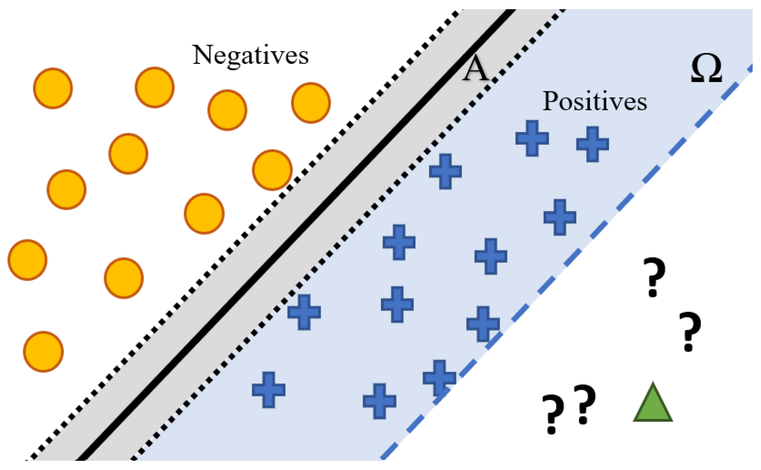
The open-set recognition problem might be difficult to comprehend when described directly for NNs, so a simple example showing binary classification in Figure 2 is provided. The decision boundary separating the positive (“+”) and negative (“o”) samples lays in the margin plane A, which is maximized during the training of the classifier. Although this is an efficient approach to distinguish between these two classes, it leads to an overgeneralization for the OSR problem. In this setting, the unknowns (“?”) and samples from unknown classes (“∆”) would be labeled as positive samples. The reason for this is that these samples are not considered when creating the boundary—it is only determined by the positive and negative samples, so there is nothing to limit the propagation of the positive label [36]. The suggested approach is to introduce the plane Ω that bounds the space of positive samples. Now, the samples that are far away in the positive half-space can be rejected by the classifier.
The formal definition of the OSR problem is given in [36] and presented here in a short form. First, the measurable recognition function f : I R d I N 0 is defined, which maps the d-dimensional input x to the label y. Next, S o is defined as a ball containing the positively labeled open space O and all positive training samples. The open space risk R O ( f ) is now defined as:
R O ( f ) = O f ( x ) d x S o f ( x ) d x ,
measuring the ratio of positively labeled open space and the overall measure of positively labeled space. Before defining the OSR problem, some instances have to be introduced. Positive training data are defined as V ^ = { v 1 , , v m } from P , and samples from other known classes K negative training data K ^ = { k 1 , , k n } . U is the set of all other unknown classes seen only in testing, hence the test set is defined as T = { t 1 , , t z } , where t i P K U . The goal is to find function f H ( H is a class of functions that separate the hyperplanes), trained on training data V ^ K ^ with given open space risk function R O ( f ) and empirical risk function R ε , such that it minimizes the open set risk:
argmin f H { R O ( f ) + λ r R ε ( f ( V ^ K ^ ) ) } ,
where λ r is the regularization constant. Now, not only is the empirical risk of the training dataset reduced, but also the open space risk associated with unknown classes U .

3.2.2. Open-Set Recognition Using NNs

The same problem persists in classification with neural networks, as samples from unknown classes are often classified with high confidence [37]. The reason for this behavior is due to the closed-set nature of NNs, i.e., the input sample is always assigned to one of the known classes. Since the final layer of the NN is softmax, the probability of the input belonging to each class is determined and the one with the highest probability is selected. However, it has been shown that there are “fooling” inputs that can lead to a high score in the classification even though they are significantly different from the rest of the samples belonging to that class [49]. Much worse, adversarial samples can also be created. These samples visually resemble those in the training dataset but result in high confidence output that is incorrect.
To address this issue, several approaches have been proposed [37]. However, one of the recent approaches that became very popular shows that if a stronger classifier is used, its open-set performance is on par with other OSR approaches. The authors of [50] concluded that a classifier’s open-set performance correlates positively with its closed-set performance across different datasets, model architectures, and objectives. However, there are certain additions to the classifier’s training procedure that allow for such performance improvement. The first is to augment the dataset with more data, as this increases the accuracy. The same effect is achieved by warming up the learning rate and smoothing the labels. The former helps with numerical instabilities at the beginning of the training, since the parameters (weights and biases) are random values that can be far from their optimal values. Hence, the learning process is started with a learning rate lower than the initial one ( η ) and gradually increased until it equals the initial rate [51]. In this work, a linear increase is used.
Since the one-hot encoded representation of the label vector y is equal to 1 at the location i = y and 0 otherwise, label smoothing affects the labels by decreasing the value of the true label for a small constant ϵ and increasing the other element values to ϵ / ( K 1 ) , where K is the number of classes:
y ^ i = 1 ϵ , if i = y , ϵ / ( K 1 ) , otherwise .
This leads to a change in the optimal solution of the loss function:
z i = log ( ( K 1 ) ( 1 ϵ ) / ϵ ) + α , if i = y , α , otherwise ,
where α is any real number. Constant ϵ affects the solution by making it finite, which is shown to increase the generalization capability [52].
It is also beneficial to train the model longer as compared to the normal setting by using the cosine learning rate decay. This decay reduces the learning rate from the initial value to zero according to the cosine law, which benefits the training progress [52]. The expression for the decay is as follows:
η t = 1 2 1 + cos t π T η ,
where η t is the learning rate at epoch t, T is the total number of epochs, and η is the initial learning rate.
Finally, the maximum logit score (MLS) is used as an open-set indicator instead of the normalized softmax score (note that MLS is used as an indicator, but softmax is used during the training and testing phase of the classifier). Logits are outputs of the penultimate layer of the NN that are given as inputs to the softmax layer. When they are normalized, the information about their magnitude, which proves to be a good indicator, is lost. Therefore, open-set detection is performed directly on logits, and in this case specifically on the logit with the highest value. Formally, MLS is defined as:
MLS ( z ) = max 1 i K z i ,
where z is a vector with prediction scores (logits) and K the number of classes.

3.3. Proposed Fault Detection Method

Considering NN classification and the problem of open-set recognition and its impact on neural networks, the proposed method uses the OSR paradigm to detect a worst-case disturbance in microgrids that cannot be detected by most conventional protection systems—a high-impedance fault. In this work, the focus is on lines connecting constant current passive loads, as this load type represents the majority in practical scenarios. The idea behind the method is to identify normal operating states of a microgrid line that connects passive load: its steady states and transients, which denote the change between the steady states, i.e., load changes. Other disturbances, in this case destructive HIFs, which should be removed from the system in the shortest time possible, are detected using an NN. However, the OSR paradigm allows these to be detected as outliers without having to model them and include them in the training dataset. Since HIFs behave differently depending on the different conditions (surface material and humidity, voltage levels, etc.), this method helps significantly in their detection [53].
The proposed HIF detection method is examined for the simplest form of NNs, the FFNN. The classifier is first trained using a standard hyperparameter tuning procedure, where the architecture of the FFNN is varied until satisfactory results are achieved and the optimizer parameters are adjusted for an efficient learning procedure. Then, the classifier is trained using the same architecture but with additional steps, as proposed in [50]. Finally, the OSR performance of the method is investigated.
The current is used as the input as transients can be detected from its waveform. It should be noted that the predominant component of DC current is the 0 Hz component, which is not useful indicator since it changes in case of both load change and HIF events. However, the difference becomes apparent when the signal is decomposed in the frequency domain using the fast Fourier transform (FFT) algorithm. The FFT algorithm is used as it is a fast solution for obtaining harmonic decomposition, especially when computation time is a crucial aspect [54]. The HIF event contains many more high-frequency components than the load change event. Hence, frequencies higher than 0 Hz are used as indicators to distinguish between the events [5]. The method should ideally distinguish between a static operating point (no transients) and load changes, flagging HIFs as outliers. The diagram of the method is provided in Figure 3.

4. Case Study

4.1. System Description

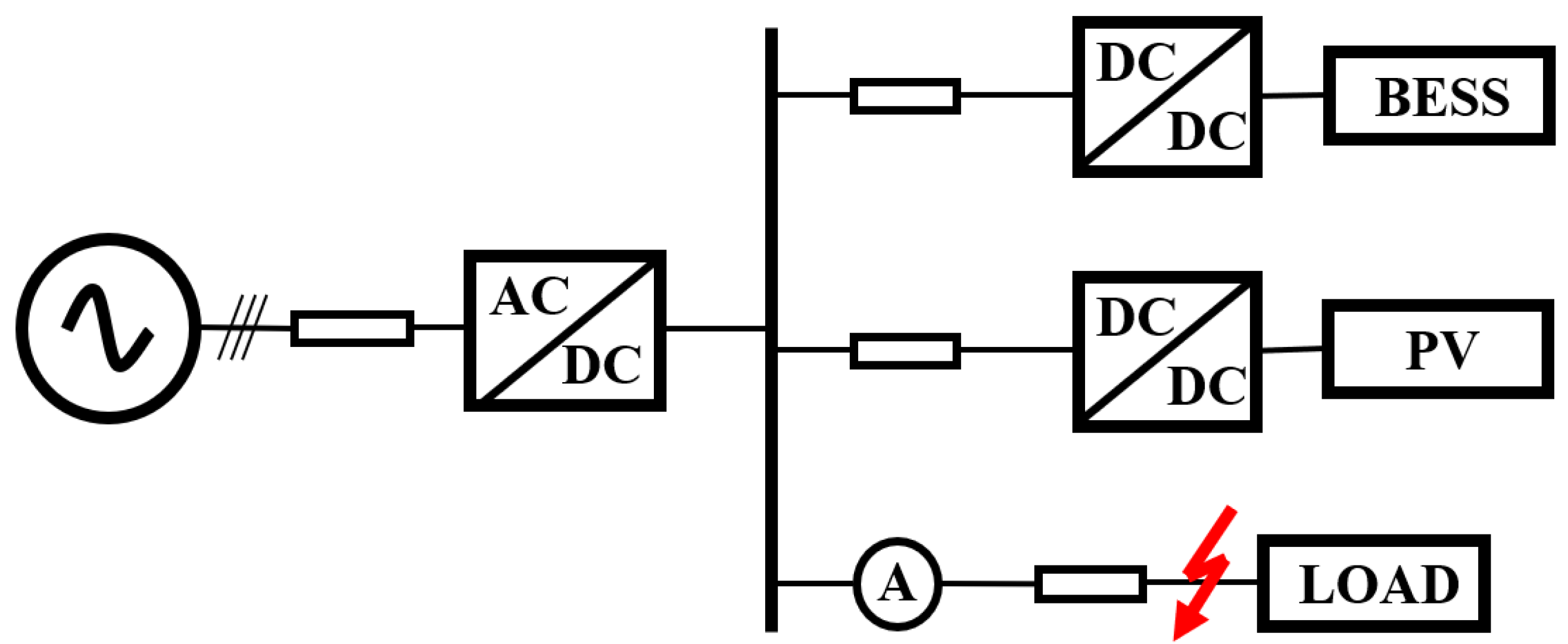
The DC microgrid system considered in this study is a renewable energy-based microgrid that includes inverter-interfaced power sources and energy storage, inspired by the DC microgrid testbed developed at the City College of New York [55]. The microgrid considered has a radial topology (a common bus) to which a photovoltaic system, battery energy storage system (BESS) and a constant current passive load are connected, as shown in Figure 4.
The PV system generates a maximum power of 6 kWp at a temperature of 25 °C. It is connected to the bus via a DC-DC boost converter with maximum power point tracking (MPPT) control, ensuring the maximum electricity output. The 12 kWh capacity BESS ensures that the excess power is stored and used when needed. The bidirectional DC-DC converter is in current control mode, enabling an effective bidirectional operation. The passive load is rated at 5 kW. The VSC connects the DC microgrid to the AC utility grid and regulates the voltage at the bus. All parameters of the microgrid are summarized in Table 1.
The current measurement for fault detection is taken at the line’s inception, denoted by the ammeter symbol, with the fault location represented by the red arrow sign. The fault location is varied along the line, ranging from 10% to 90% of the line length.

4.2. Dataset

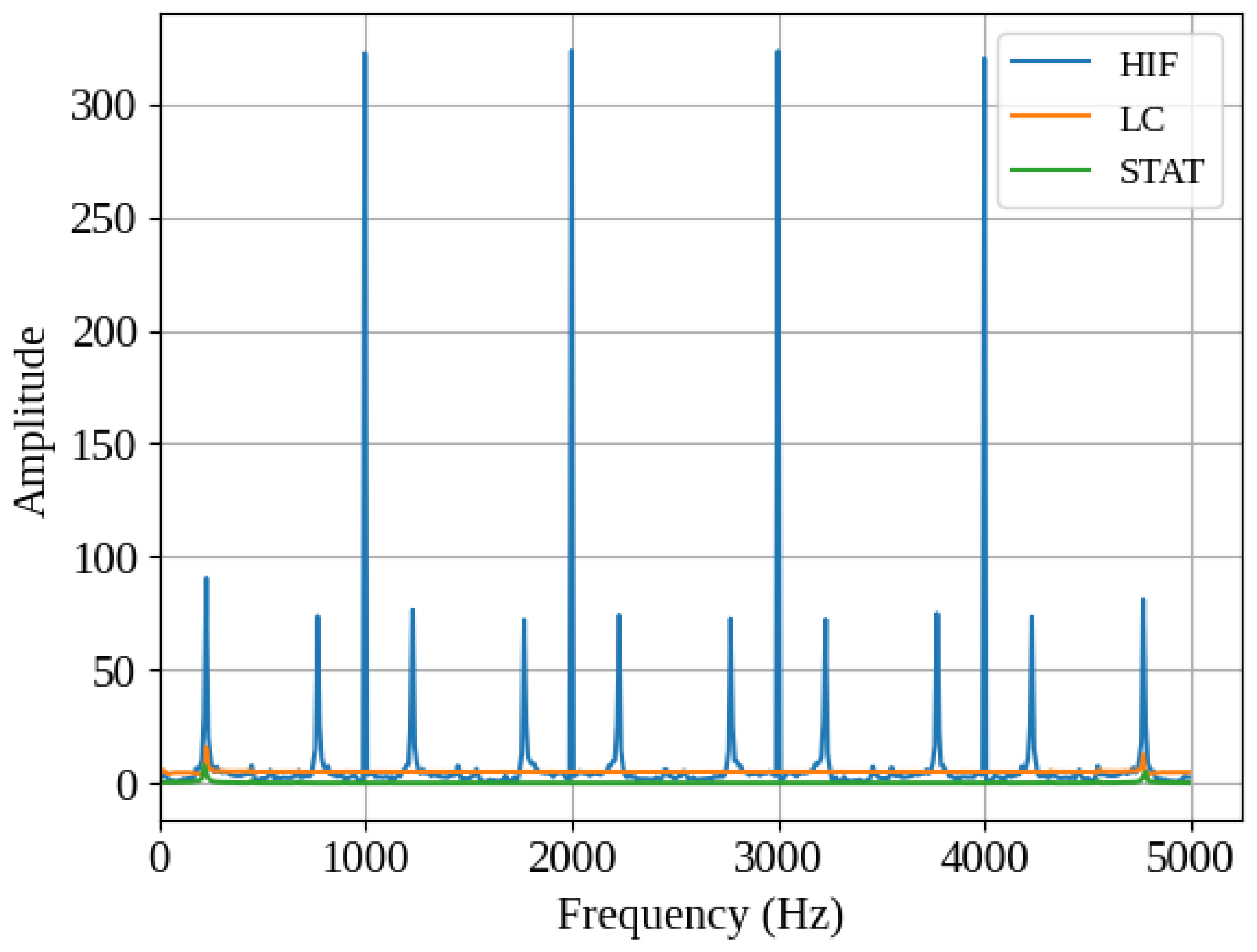
The dataset includes various types of events, each represented by time series of current measurements, with a length of 1000 samples. These measurements are taken at the beginning of the line connecting passive load to the bus. Since the sampling frequency used is 10 kHz, the time duration of each time series is 100 ms, which is sufficient to capture the transients of interest. The elementary state of the microgrid is a steady state in which the current is flat with ripples originating from converter operations, and this state is included in the dataset. Load changes, such as the increase/decrease in generation or load, are also included. Finally, the responses of the microgrid to HIFs with different parameters are collected for testing of the method. The first two classes are used for training the classifier. The unknown class, in this case the HIF, is also included to test the OSR performance of the classifiers, but they are not seen by the classifier during the training procedure. Gaussian noise with zero mean and standard deviation of 0.01, is added to better approximate the real-world response. The entire dataset, without noise, can be found in the online repository [56]. The dataset contains 200 waveforms of normal operation and 21 HIF responses. A representative of each event is depicted in Figure 5. If the load is in its stationary state, the current remains flat throughout the entire window. Non-stationary events occur at t = 0. After the load change, the current reaches a new steady state. However, during HIF, even though a new steady state is achieved, the arcing phenomenon is clearly visible in time and frequency domains (Figure 6). The amplitudes that HIF achieves at high frequencies surpass those of stationary state and load change, thereby revealing a distinct difference.
It is worth noting that standards for arc fault protection in PV systems exist, each defining the arc type, conductor size, fault location, and other requirements [57]. Even though subject of this research is a line that connects a passive load, the authors created dataset according to the IEC 63027 standard while also incorporating additional fault locations and current levels, as suggested in [58]. However, this aspect will be emphasized in future work, where the method will undergo experimental testing.
During data preprocessing, each event occurrence is shifted in time to better represent the different times the event could appear and to augment the training data. Subsequently, each sequence is transformed from the time domain to the frequency domain using the fast Fourier transform (FFT), and the absolute value is taken. To simplify, the values at negative frequencies are added to their positive counterparts, and the dominant zero-frequency component is removed by zero multiplication. This reduces the input dimensionality to 500. Finally, the dataset is standardized. The two classes representing the stationary state and load change are encoded with numbers 0 and 1, respectively. The dataset is designed to serve as an example of the OSR problem but can also be used to test any HIF detection method.

4.3. Results

The FFNN is used because its architecture is simple and the training procedure is relatively straightforward. The FFNN is first trained to achieve the best possible accuracy (defined as ratio of correctly classified samples and total number of samples) on the test dataset. The second FFNN, with the same architecture, is trained but with improvements that aim to increase its open-set performance. The FFNN is set to take 500 points as inputs, as this is the size of the transform of the time sequence that describes an event, as explained before. The input layer is followed by three linear layers with sizes 2000, 2000, and 400, each of which has a Rectified Linear Unit (ReLU) nonlinearity at its output. The number of nodes in the first hidden layer is selected to increase the dimensionality of the input. The second hidden layer retains the same number of nodes, as iterative parameter selection indicated that further increases in dimensionality did not enhance the neural network’s performance. The third hidden layer reduces dimensionality before the final reduction in the output layer. The number of nodes in this layer is reduced by a factor of five compared to the previous hidden layer, as the iterative parameter selection process demonstrated that this achieves an optimal balance between the neural network’s complexity and accuracy. The final linear layer reduces the size from 400 to a vector of size 2, with each element representing a class. The ReLU nonlinear function is applied at the output of each hidden layer, as it is computationally efficient and avoids the vanishing gradient problem encountered with other nonlinear functions, such as the sigmoid function. A batch size of 32 samples is used, as it provides a good balance between convergence speed and the neural network’s generalization ability. This same rationale guided the selection of the learning rate and number of epochs. Additionally, RMSprop is employed as the optimizer due to its ability to ensure stable convergence, even in cases with sparse gradients. Both the learning rate warmup and label smoothing were determined iteratively in alignment with the OSR framework. The architectures for both classifiers, as well as other parameters and the optimizer used, can be found in Table 2.
As can be seen from the table, the only difference between the classifiers is in the improvements related to the OSR performance. Instead of a fixed value, the cosine learning rate with warmup was used, which means that the learning rate is increased from 1 × 10⁻⁴ to 1 × 10⁻³ during the first 10% of the total number of epochs. After it reaches its maximum, it is reduced for the remaining number of epochs according to the cosine law. The accuracy of the classifier is not reduced after applying all OSR rules, and the learning process converges as shown in Figure 7.
The reason for using MLS becomes clearer when dealing with unknown samples that are not part of the dataset, in this case HIFs. The standard approach is that for each input sample, the classifier produces a vector of size equal to the number of classes. The vector elements are normalized using the softmax function to obtain probabilities of the input belonging to each class; i.e., each vector element is in the range [0, 1] and their sum is equal to 1. However, this approach does not take into account the vector amplitude information, which is extremely useful when working with unknowns. Therefore, the MLS approach is used to detect HIFs. The output of the classifier is not softmaxed, but the maximum element of this vector is used to represent the class.
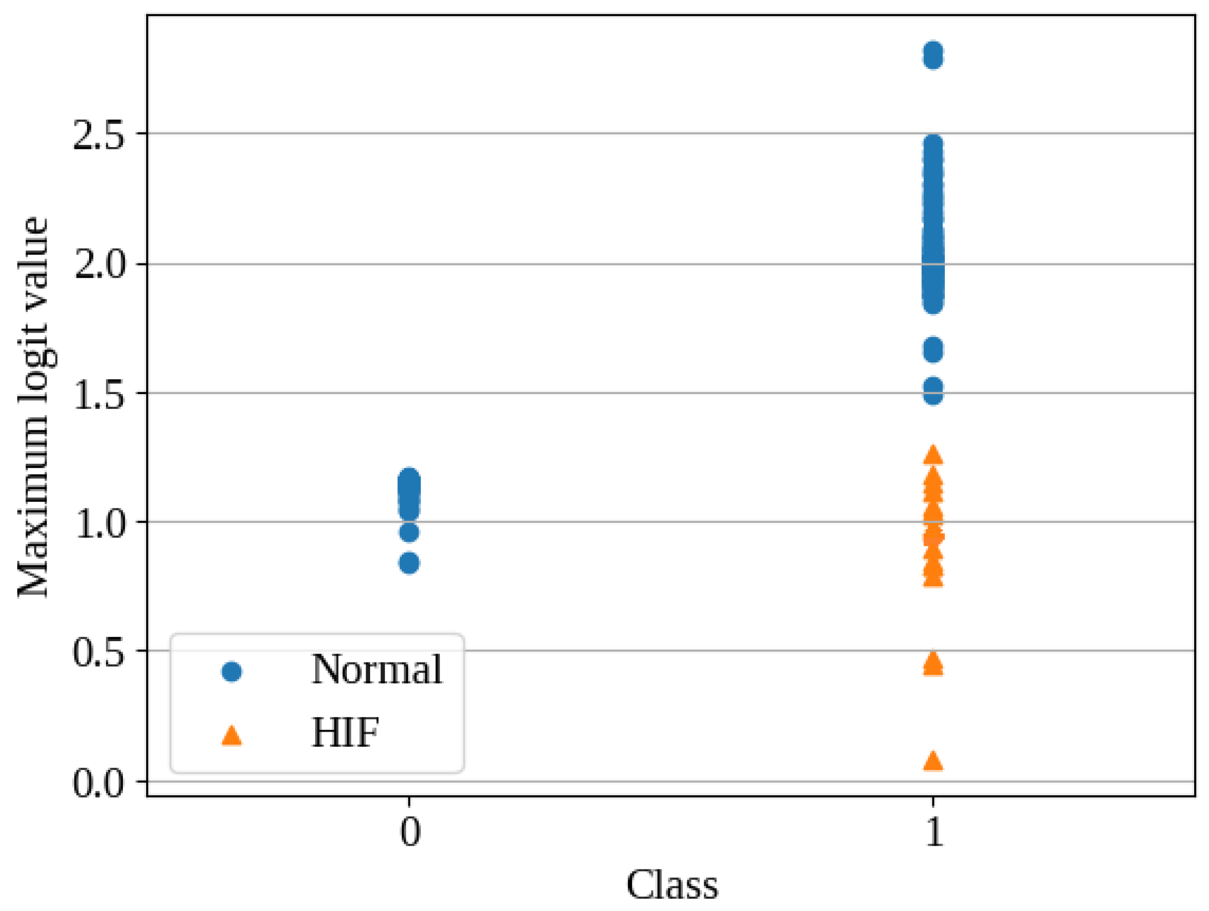
The FFNN and the FFNN with OSR enhancements are fed the same test and HIF samples. Figure 8 and Figure 9 show the maximum logits of the test samples and the HIFs. (blue dots and orange triangles, respectively).
The MLSs of the steady-state class (0) for FFNN without improvements are closely spaced, but for the load change class (1) they are widely scattered (Figure 8). The latter discrepancy arises from differences in the directions in which load changes occur, as well as variations in the magnitudes of load changes. The features characterizing steady states are similar, with the only difference being the 0 Hz component (representing different loading levels), which is removed during preprocessing. As expected, HIFs are misclassified because the NN always assigns a class to the inputs. Furthermore, the NN assigns HIFs to both classes, even though the HIF response is more similar to that of load change. Moreover, the MLSs of known classes and the HIF overlap, indicating that the classifier struggles to handle unknowns effectively.
On the other hand, the results for the FFNN trained according to the OSR suggestions are shown in Figure 9. The scale of the logits shrank on the y-axis, but now the samples of both classes are grouped. The NN decided correctly that these samples are closer to the load change event than to the steady state, assigning all the HIFs to the class 1. More importantly, the MLSs of the HIFs are far from the rest of the MLSs, indicating that the input is from the unknown class. Thus, the HIF can be identified as an outlier and rejected by the classifier in a trivial manner.
The OSR approach proves valuable in detecting outliers. The neural network, with these additions to the training procedure, demnostrates an enhanced ability to detect outliers in a straightforward manner.

4.4. Comparison with Existing NN-Based Methods

This section compares the proposed method with other neural network-based approaches, evaluating their performance in terms of complexity, computational efficiency, and detection accuracy. The comparison is limited to NN-based methods, as they closely align with the framework of the proposed approach. This focused evaluation enables a meaningful assessment of the relative strengths and limitations. Furthermore, it highlights the advancements and contributions of the proposed method within this specific context.
Table 3 presents several approaches based on different types of neural networks, all tested on the same dataset used to evaluate the proposed method. The proposed method achieves the highest detection accuracy (99.99) among all methods, demonstrating its performance while maintaining low complexity. Both the proposed method and the approach in [32] exhibit high computational efficiency; however, the proposed method significantly outperforms [32] in terms of the detection accuracy (99.99% vs. 70.09%). In terms of complexity, while the CNN-based method in [31] achieves high detection accuracy (96.79%), it suffers from high complexity, making it less suitable for resource-constrained or real-time applications. The back-propagation neural network (BPNN)-based method in [30] offers a balance between medium complexity and high efficiency but falls short in accuracy (95.31%) compared to the proposed method. Finally, unlike all other methods, the proposed method supports OSR, making it robust and adaptable to scenarios involving unknown or unexpected faults. This capability provides a significant advantage over other approaches.

4.5. Fault Detection Algorithm

The OSR improved performance of the NN, allowing it to be used not only as a classifier but also as an outlier detector (HIFs in this case). Algorithm 1 summarizes the fault detection method. The offline part of the algorithm consists of the dataset creation, the classifier training, and determining the bounds of the samples per class. The bounds can be chosen in any manner that separates outliers. In this work, a fixed bound for both classes is proposed, but other methods can be used instead. The goal of the bounds is to capture the range in which the normal samples for that class occur. In the case shown in Figure 9, the bound for both classes could be any number below the lowest scoring sample of each class. Anything under this limit is considered an outlier.
Algorithm 1 High-impedance fault detection
OFFLINE
  •   1. Obtain dataset with normal operating conditions
          (steady state, load changes)
  •   2. Transform data from time to frequency domain
          using FFT algorithm
  •   3. Train NN-based classifier C with OSR suggestions
  •   4. Obtain responses to HIFs
  •   5. Find MLS for normal samples (test set) and HIFs
  •   6. Determine boundaries that enclose normal samples
          of each class
ONLINE
  •   1. Take N consecutive samples of current
          measurement and create vector X
  •   2. Find MLS and assigned class k from C ( X )
  •   3. if MLS outside boundaries for class k:
          HIF detected.
  •   4. else return to step 1.
The online part describes how fault detection works. The method requires passing a vector of length N, in this case 500, to the pre-trained classifier. The output of the classifier contains logits from which the maximum (MLS) is determined, along with the class that the classifier assigned to the input. The assigned class specifies the bounds against which the MLS is to be compared. If the MLS is outside the bounds, it is declared an outlier, in this case an HIF. If it is not, X is updated.

4.6. Discussion

The goal of this study is to develop an HIF detection method that is based on an NN trained according to the OSR suggestions. These suggestions allow unknowns (inputs that are not seen by the classifier during its training—in this case HIFs) to be treated as outliers. The first advantage of this approach is that the HIF responses do not need to be included in the dataset, which relieves the user of the need to model HIFs and reduces complexity of the classifier (NN). This is achieved because both the FFNN and the CNN classifiers have simple architectures but can still properly handle unknowns, making it possible to set bounds around the correctly classified samples. Consequently, the detection of outliers (HIFs) is simple—it is enough to check whether the MLS of an input is outside the bounds of the class assigned by the classifier. It should be noted that it cannot be known a priori which class an input will be assigned to, so the MLS is compared to the bounds of the class into which the classifier has placed it. This is the general case, but it may happen that the same bounds can be applied to both classes, so it is not necessary to know which class the classifier has assigned to the input. The bounds do not have to be fixed, as any strategy can be used to detect outliers. In this work, the fixed bound is used for simplicity.
Speaking of disturbances other than HIFs, some characteristics could be included in the dataset, but it is difficult to know and model all the disturbances that occur in a microgrid. It is assumed here that the HIF response is specific and different from that of other disturbances. Moreover, 100 ms is long enough that temporary disturbances do not trigger the trip signal, while HIFs, on the other hand, persist. At the time of writing, the authors are not aware that a dataset for HIF detection exists. Since the dataset is publicly available, it can be used as a basis for further research. Any improvements to the dataset and method are encouraged. Future work can be based on any of the above: enhancing the dataset by including more normal operating points or adding real-world HIF responses, improving the classifiers or the training procedure, or treating outliers differently. Testing the method on real-world data would increase pressure on classifier’s discriminative capabilities, potentially raising the need for input filtering, using different signal decomposition methods (e.g., wavelet transform), or incorporation of additional input features. One of the research directions could cover adaptation of the proposed method for lines that connect power sources, energy storage systems or active loads, as it is currently limited to lines connecting passive loads. Another research direction could investigate applying the method to long DC lines, such as those used in HVDC transmission systems.
It is also worth noting that hardware could be a limiting factor, as the method requires implementation of the neural network on the processor. This involves handling fast matrix multiplication and implementation of nonlinear functions, which must be carefully managed to minimize computational overhead and ensure fast execution. Both factors impact the neural network’s classification performance, which, in turn, directly affects the fault detection performance [59,60].

5. Conclusions

Detecting high-impedance faults is a challenging task for conventional protection systems due to their low current magnitude. However, advanced intelligent classifiers are capable of detecting repetitive patterns that characterize such faults. In this work, we present an HIF detection method based on intelligent classification, using a feed-forward neural network as the classifier. The FFNN is trained to distinguish normal operating points (knowns) from unknowns, which in this case are identified as HIFs and treated as outliers. The key conclusions drawn from this study are as follows: (i) the number of classes in the dataset can be reduced by focusing on normal operating states; (ii) HIFs can be detected as outliers using a neural network trained according to open-set recognition principles; (iii) the architecture of the neural network does not need modification, only the training procedure; (iv) FFNNs are highly effective for HIF detection, with an accuracy of 99.99%. Additionally, the dataset used in this study is made publicly available, as no similar datasets exist in the literature. This method offers a promising approach for improving fault detection in power grids, especially in microgrids and other low-current scenarios.

Author Contributions

Conceptualization, I.G. and H.P.; methodology, I.G. and H.P.; validation, I.G.; formal analysis, I.G.; resources, H.P.; data curation, I.G.; writing—original draft preparation, I.G.; writing—review and editing, H.P.; visualization, I.G.; supervision, H.P. All authors have read and agreed to the published version of the manuscript.

Funding

This research received no external funding.

Institutional Review Board Statement

Not applicable.

Informed Consent Statement

Not applicable.

Data Availability Statement

The data used to support the findings of this study are available from the corresponding author upon request.

Conflicts of Interest

The authors declare no conflicts of interest.

Abbreviations

The following abbreviations are used in this manuscript:
ACAlternating current
BESSBattery energy storage system
BPNNBack-propagation neural network
CNNConvolutional neural network
DCDirect current
DERDistributed energy sources
DWTDiscrete wavelet transform
FFNNFeed-forward neural network
FFTFast Fourier transform
GANGenerative adversarial network
HIFHigh-impedance fault
kNNk-Nearest neighbors
LIFLow-impedance fault
MLSMaximum logit score
MPPTMaximum power point tracking
NNNeural network
OSROpen-set recognition
PVPhoto-voltaic
ReLURectified linear unit
RNNRecurrent neural network
RESRenewable energy sources
SVMSupport vector machine
VSCVoltage source converter

References

  1. Muhtadi, A.; Pandit, D.; Nguyen, N.; Mitra, J. Distributed Energy Resources Based Microgrid: Review of Architecture, Control, and Reliability. IEEE Trans. Ind. Appl. 2021, 57, 2223–2235. [Google Scholar] [CrossRef]
  2. Hatziargyriou, N.; Asano, H.; Iravani, R.; Marnay, C. Microgrids. IEEE Power Energy Mag. 2007, 5, 78–94. [Google Scholar] [CrossRef]
  3. Papadimitriou, C.N.; Zountouridou, E.I.; Hatziargyriou, N.D. Review of hierarchical control in DC microgrids. Electr. Power Syst. Res. 2015, 122, 159–167. [Google Scholar] [CrossRef]
  4. Ansari, S.; Chandel, A.; Tariq, M. A Comprehensive Review on Power Converters Control and Control Strategies of AC/DC Microgrid. IEEE Access 2021, 9, 17998–18015. [Google Scholar] [CrossRef]
  5. Grcić, I.; Pandžić, H.; Novosel, D. Fault Detection in DC Microgrids Using Short-Time Fourier Transform. Energies 2021, 14, 277. [Google Scholar] [CrossRef]
  6. Čuljak, M.; Pandžić, H.; Havelka, J. Mathematical Morphology-Based Fault Detection in Radial DC Microgrids Considering Fault Current from VSC. IEEE Trans. Smart Grid 2023, 14, 2545–2557. [Google Scholar] [CrossRef]
  7. Grcić, I.; Pandžixcx, H. Fault Detection in DC Microgrids using Recurrent Neural Networks. In Proceedings of the 2021 International Conference on Smart Energy Systems and Technologies (SEST), Vaasa, Finland, 6–8 September 2021; pp. 1–6. [Google Scholar]
  8. Ali, Z.; Terriche, Y.; Abbas, S.Z.; Hassan, M.A.; Sadiq, M.; Su, C.L.; Guerrero, J.M. Fault Management in DC Microgrids: A Review of Challenges, Countermeasures, and Future Research Trends. IEEE Access 2021, 9, 128032–128054. [Google Scholar] [CrossRef]
  9. Yao, X.; Wang, J.; Schweickart, D.L. Review and recent developments in DC arc fault detection. In Proceedings of the 2016 IEEE International Power Modulator and High Voltage Conference (IPMHVC), San Francisco, CA, USA, 6–9 July 2016; pp. 467–472. [Google Scholar]
  10. Dhar, S.; Patnaik, R.K.; Dash, P.K. Fault Detection and Location of Photovoltaic Based DC Microgrid Using Differential Protection Strategy. IEEE Trans. Smart Grid 2018, 9, 4303–4312. [Google Scholar] [CrossRef]
  11. Wang, Y.; Hou, L.; Paul, K.C.; Ban, Y.; Chen, C.; Zhao, T. ArcNet: Series AC Arc Fault Detection Based on Raw Current and Convolutional Neural Network. IEEE Trans. Ind. Inform. 2022, 18, 77–86. [Google Scholar] [CrossRef]
  12. Paz, F.; Ordonez, M. High-Impedance Fault Detection Method for DC Microgrids. In Proceedings of the 2019 IEEE 10th International Symposium on Power Electronics for Distributed Generation Systems (PEDG), Xi’an, China, 3–6 June 2019; pp. 787–792. [Google Scholar]
  13. Taheri, B.; Hosseini, S.A. Detection of High Impedance Fault in DC Microgrid Using Impedance Prediction Technique. In Proceedings of the 2020 15th International Conference on Protection and Automation of Power Systems (IPAPS), Shiraz, Iran, 30–31 December 2020; pp. 68–73. [Google Scholar]
  14. Sheikh, A.A.; Wakode, S.A.; Deshmukh, R.R.; Ballal, M.S. Detection of High Impedance Fault in DC Microgrid. In Proceedings of the 2020 IEEE International Conference on Power Electronics, Drives and Energy Systems (PEDES), Jaipur, India, 16–19 December 2020; pp. 1–4. [Google Scholar]
  15. Rao, G.K.; Jena, P. Fault Detection in DC Microgrid Based on the Resistance Estimation. IEEE Syst. J. 2022, 16, 1009–1020. [Google Scholar] [CrossRef]
  16. Stanescu, D.; Digulescu, A.; Ioana, C.; Serbanescu, A.; Zhang, Y.D.; Senjyu, T.; So-In, C.; Joshi, A. On the Existing and New Potential Methods for Partial Discharge Source Monitoring in Electrical Power Grids. In Smart Trends in Computing and Communications; Lecture Notes in Networks and Systems; Springer: Singapore, 2022; Volume 286. [Google Scholar]
  17. Stanescu, D.; Digulescu, A.; Ioana, C.; Serbanescu, A. Entropy-Based Characterization of the Transient Phenomena—Systemic Approach. Mathematics 2021, 9, 648. [Google Scholar] [CrossRef]
  18. Srivastava, C.; Tripathy, M. Novel Grounding and Protection Strategy for DC Microgrid Restraining Fault Current. IEEE Trans. Power Deliv. 2024, 39, 2182–2193. [Google Scholar] [CrossRef]
  19. Miao, W.; Wang, Z.; Wang, F.; Lam, K.H.; Pong, P.W.T. Multicharacteristics Arc Model and Autocorrelation-Algorithm Based Arc Fault Detector for DC Microgrid. IEEE Trans. Ind. Electron. 2023, 70, 4875–4886. [Google Scholar] [CrossRef]
  20. Valero, A. High Impedance Fault Detection Method in Multi-Grounded Distribution Networks. Ph.D. Dissertation, École polytechnique de Bruxelles Université Libre de Bruxelles, Brussels, Belgium, 2012. [Google Scholar]
  21. Masa, A.V.; Werben, S.; Maun, J.C. Incorporation of data-mining in protection technology for high impedance fault detection. In Proceedings of the 2012 IEEE Power and Energy Society General Meeting, San Diego, CA, USA, 22–26 July 2012; pp. 1–8. [Google Scholar]
  22. Subramaniam, K.; Illindala, M.S. High Impedance Fault Detection and Isolation in DC Microgrids. In Proceedings of the 2019 IEEE/IAS 55th Industrial and Commercial Power Systems Technical Conference (I&CPS), Calgary, AB, Canada, 5–8 May 2019; pp. 1–8. [Google Scholar]
  23. Wakode, S.A.; Kumar, S.; Ballal, M.S. A Flexible Protection Approach for DC Microgrid Using Wavelet based Machine Learning Technique. In Proceedings of the 2021 IEEE 2nd International Conference on Smart Technologies for Power, Energy and Control (STPEC), Bilaspur, Chhattisgarh, India, 19–22 December 2021; pp. 1–5. [Google Scholar]
  24. Bramareswara Rao, S.N.V.; Kumar, Y.V.P.; Amir, M.; Muyeen, S.M. Fault detection and classification in hybrid energy-based multi-area grid-connected microgrid clusters using discrete wavelet transform with deep neural networks. Electr. Eng. 2024. [Google Scholar] [CrossRef]
  25. Taheri, B.; Hosseini, S.A.; Salehimehr, S.; Razavi, F. A Novel Approach for Detection High Impedance Fault in DC Microgrid. In Proceedings of the 2019 International Power System Conference (PSC), Tehran, Iran, 9–11 December 2019; pp. 287–292. [Google Scholar]
  26. Grcić, I.; Pandžić, H. Artificial Neural Network for High-Impedance-Fault Detection in DC Microgrids. In Proceedings of the 2023 IEEE PES Conference on Innovative Smart Grid Technologies—Middle East (ISGT Middle East), Abu Dhabi, United Arab Emirates, 12–15 March 2023; pp. 1–5. [Google Scholar]
  27. Aziz, F.; Haq, A.U.; Ahmad, S.; Mahmoud, Y.; Jalal, M.; Ali, U. A Novel Convolutional Neural Network-Based Approach for Fault Classification in Photovoltaic Arrays. IEEE Access 2020, 8, 41889–41904. [Google Scholar] [CrossRef]
  28. Lu, S.; Sirojan, T.; Phung, B.T.; Zhang, D.; Ambikairajah, E. DA-DCGAN: An Effective Methodology for DC Series Arc Fault Diagnosis in Photovoltaic Systems. IEEE Access 2019, 7, 45831–45840. [Google Scholar] [CrossRef]
  29. Veerasamy, V.; Wahab, N.I.A.; Othman, M.L.; Padmanaban, S.; Sekar, K.; Ramachandran, R.; Hizam, H.; Vinayagam, A.; Islam, M.Z. LSTM Recurrent Neural Network Classifier for High Impedance Fault Detection in Solar PV Integrated Power System. IEEE Access 2021, 9, 32672–32687. [Google Scholar] [CrossRef]
  30. Yang, J.; Wang, Y. Identification and Detection of DC Arc Fault in Photovoltaic Power Generation System. In Proceedings of the 2020 International Conference on Intelligent Transportation, Big Data & Smart City (ICITBS), Vientiane, Laos, 11–12 January 2020; pp. 440–444. [Google Scholar]
  31. Omran, A.H.; Said, D.M.; Hussin, S.M.; Mirsaeidi, S.; Abid, Y.M. An Intelligent Classification Method of Series Arc Fault Models Using Deep Learning Algorithm. In Proceedings of the 2020 IEEE International Conference on Power and Energy (PECon), Penang, Malaysia, 21–24 July 2020; pp. 44–48. [Google Scholar]
  32. Patil, D.D.; Bindu, S.; SushilThale. Arc Fault Detection in DC Microgrid Using Deep Neural Network. In Proceedings of the 2021 4th Biennial International Conference on Nascent Technologies in Engineering (ICNTE), NaviMumbai, India, 15–16 January 2021; pp. 1–6. [Google Scholar]
  33. Cai, X.; Wai, R.-J. Intelligent DC Arc-Fault Detection of Solar PV Power Generation System via Optimized VMD-Based Signal Processing and PSO–SVM Classifier. IEEE J. Photovolt. 2022, 12, 1058–1077. [Google Scholar] [CrossRef]
  34. Lu, S.; Sahoo, A.; Ma, R.; Phung, B.T. DC Series Arc Fault Detection Using Machine Learning in Photovoltaic Systems: Recent Developments and Challenges. In Proceedings of the 2020 8th International Conference on Condition Monitoring and Diagnosis (CMD), Phuket, Thailand, 25–28 October 2020; pp. 416–421. [Google Scholar]
  35. Mansouri, M.; Trabelsi, M.; Nounou, H.; Nounou, M. Deep Learning-Based Fault Diagnosis of Photovoltaic Systems: A Comprehensive Review and Enhancement Prospects. IEEE Access 2021, 9, 126286–126306. [Google Scholar] [CrossRef]
  36. Scheirer, W.J.; de Rezende Rocha, A.; Sapkota, A.; Boult, T.E. Toward Open Set Recognition. IEEE Trans. Pattern Anal. Mach. Intell. 2013, 35, 1757–1772. [Google Scholar] [CrossRef]
  37. Bendale, A.; Boult, T.E. Towards Open Set Deep Networks. In Proceedings of the 2016 IEEE Conference on Computer Vision and Pattern Recognition (CVPR), Las Vegas, NV, USA, 27–30 June 2016; pp. 1563–1572. [Google Scholar]
  38. Geng, C.; Huang, S.-J.; Chen, S. Recent Advances in Open Set Recognition: A Survey. IEEE Trans. Pattern Anal. Mach. Intell. 2021, 43, 3614–3631. [Google Scholar] [CrossRef] [PubMed]
  39. Beheshtaein, S.; Cuzner, R.M.; Forouzesh, M.; Savaghebi, M.; Guerrero, J.M. DC Microgrid Protection: A Comprehensive Review. IEEE J. Emerg. Sel. Top. Power Electron. 2019; early access. [Google Scholar]
  40. Bayati, N. Fault Detection and Location of DC Microgrids. Ph.D. Dissertation, Faculty of Engineering and Science, Aalborg University, Aalborg, Denmark, 2020. [Google Scholar]
  41. Li, J.; Kohler, J.L. New insight into the detection of high-impedance arcing faults on DC trolley systems. IEEE Trans. Ind. Appl. 1999, 35, 1169–1173. [Google Scholar]
  42. Bayati, N.; Savaghebi, M. A high-impedance fault detection scheme for DC aircrafts based on comb filter and second derivative of voltage. Green Energy Intell. Transp. 2023, 2, 100073. [Google Scholar] [CrossRef]
  43. Oh, Y.; Kim, C.; Gwon, G.; Noh, C.; Bukhari, S.; Haider, R.; Gush, T. Fault detection scheme based on mathematical morphology in last mile radial low voltage DC distribution networks. Int. J. Electr. Power Energy Syst. 2019, 106, 520–527. [Google Scholar] [CrossRef]
  44. Andrea, J.; Schweitzer, P.; Tisserand, E. A New DC and AC Arc Fault Electrical Model. In Proceedings of the 2010 56th IEEE Holm Conference on Electrical Contacts, Charleston, SC, USA, 4–7 October 2010; pp. 1–6. [Google Scholar]
  45. Yadav, N.; Tummuru, N.R. Short-Circuit Fault Detection and Isolation Using Filter Capacitor Current Signature in Low-Voltage DC Microgrid Applications. IEEE Trans. Ind. Electron. 2022, 69, 8491–8500. [Google Scholar] [CrossRef]
  46. Goodfellow, I.; Bengio, Y.; Courville, A. Deep Learning; MIT Press: Cambridge, MA, USA, 2016. [Google Scholar]
  47. Gu, J.; Wang, Z.; Kuen, J.; Ma, L.; Shahroudy, A.; Shuai, B.; Liu, T.; Wang, X.; Wang, G.; Cai, J.; et al. Recent advances in convolutional neural networks. Pattern Recognition 2018, 77, 354–377. [Google Scholar] [CrossRef]
  48. Hüsken, M.; Stagge, P. Recurrent neural networks for time series classification. Neurocomputing 2003, 50, 223–235. [Google Scholar] [CrossRef]
  49. Nguyen, A.; Yosinski, J.; Clune, J. Deep neural networks are easily fooled: High confidence predictions for unrecognizable images. In Proceedings of the 2015 IEEE Conference on Computer Vision and Pattern Recognition (CVPR), Boston, MA, USA, 7–12 June 2015; pp. 427–436. [Google Scholar]
  50. Vaze, S.; Han, K.; Vedaldi, A.; Zisserman, A. Open-Set Recognition: A Good Closed-Set Classifier is All You Need. In Proceedings of the Tenth International Conference on Learning Representations (ICLR), Virtual Event, 25–29 April 2022; pp. 1–26. [Google Scholar]
  51. He, K.; Zhang, X.; Ren, S.; Sun, J. Deep Residual Learning for Image Recognition. In Proceedings of the 2016 IEEE Conference on Computer Vision and Pattern Recognition (CVPR), Las Vegas, NV, USA, 27–30 June 2016; pp. 770–778. [Google Scholar]
  52. He, T.; Zhang, Z.; Zhang, H.; Zhang, Z.; Xie, J.; Li, M. Bag of Tricks for Image Classification with Convolutional Neural Networks. In Proceedings of the 2019 IEEE/CVF Conference on Computer Vision and Pattern Recognition (CVPR), Long Beach, CA, USA, 15–20 June 2019; pp. 558–567. [Google Scholar]
  53. Ghaderi, A.; Ginn, H.L.; Mohammadpour, H.A. High impedance fault detection: A review. Electr. Power Syst. Res. 2017, 143, 376–388. [Google Scholar] [CrossRef]
  54. Saribulut, L.; Teke, A.; Tumay, M. Fundamentals and literature review of Fourier transform in power quality issues. J. Electr. Electron. Eng. Res. 2013, 5, 9–22. [Google Scholar]
  55. Saleh, M.; Esa, Y.; Mhandi, Y.; Brandauer, W.; Mohamed, A. Design and implementation of CCNY DC microgrid testbed. In Proceedings of the 2016 IEEE Industry Applications Society Annual Meeting, Portland, OR, USA, 2–6 October 2016; pp. 1–7. [Google Scholar]
  56. Grcić, I. Dataset HIF Detection [Data Set]. Available online: https://github.com/ivangrcic/dataset-hif-detection (accessed on 15 November 2024.).
  57. Putzke, J.L.; Michels, L.; Bellinaso, L.V. Electric Arcs in Photovoltaic Systems: A Comparative Analysis of IEC 63027, UL 1699B, and GB-t 39750 Standards. In Proceedings of the 2023 IEEE 8th Southern Power Electronics Conference and 17th Brazilian Power Electronics Conference (SPEC/COBEP), Florianopolis, Brazil, 26–29 November 2023; pp. 1–5. [Google Scholar]
  58. Wang, Y.; Zhou, J.; Paul, K.C.; Zhao, T.; Sheng, D. Explainability Approach-Based Series Arc Fault Detection Method for Photovoltaic Systems. IEEE Access 2024, 12, 45530–45542. [Google Scholar] [CrossRef]
  59. Zhang, Z.; Li, J. A Review of Artificial Intelligence in Embedded Systems. Micromachines 2023, 14, 897. [Google Scholar] [CrossRef] [PubMed]
  60. Capra, M.; Bussolino, B.; Marchisio, A.; Shafique, M.; Masera, G.; Martina, M. An Updated Survey of Efficient Hardware Architectures for Accelerating Deep Convolutional Neural Networks. Future Internet 2020, 12, 113. [Google Scholar] [CrossRef]
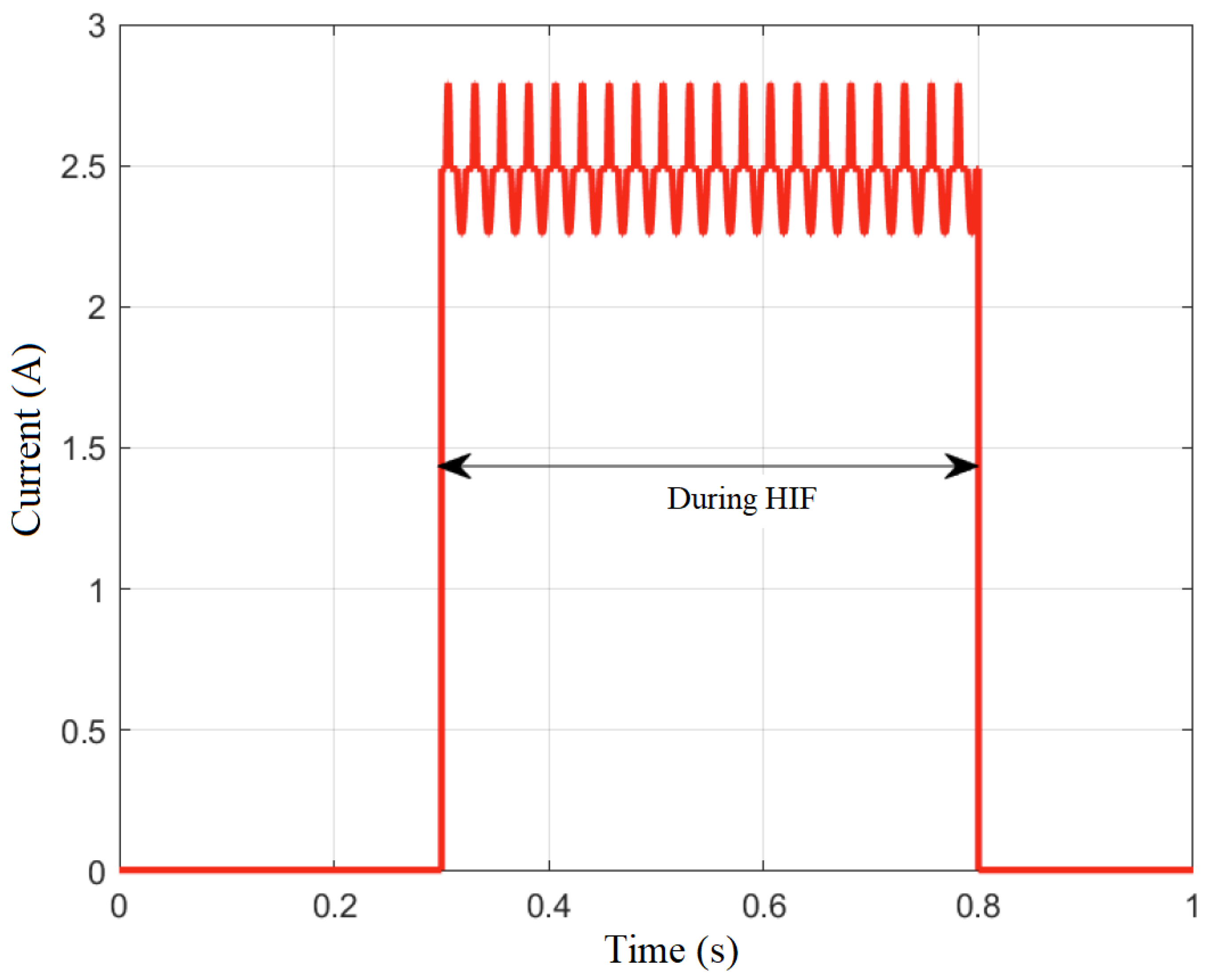
Figure 1. Fault current of the HIF model. The fault buildup starts at t = 0.3 s and lasts until the current reaches its maximum magnitude and is followed by the shoulder. The nonlinear stage lasts until the fault is cleared at t = 0.8 s.
Applsci 15 00193 g001
Figure 2. Illustration of the open-set recognition problem. Plane A separates the sample space into two half-spaces, so that unknowns (“?”) and samples from unknown classes (“∆”) are part of the positive sample space. The second plane Ω is added to limit the open space risk by restricting the positive sample space. In case of fault detection, negative samples are steady states and positive samples are load changes. The unknowns and unknown classes are HIFs and other disturbances that occur in the microgrid.
Applsci 15 00193 g002
Figure 3. Overview of the proposed fault detection method, where, based on the FFT of the current, an intelligent classifier decides whether the event is known (and to which class it belongs) or not.
Applsci 15 00193 g003
Figure 4. Simulation model of a DC microgrid. Model includes battery energy storage system, PV module, passive load, and utility grid connection. The fault location is on the line that connects load to the bus.
Applsci 15 00193 g004
Figure 5. Representatives of dataset classes (steady state, load change) and HIF in the time domain. The stationary current is flat with ripples, while the load change current transitions to another steady state after a transient period. Notably, the arcing phenomenon is clearly visible during the HIF.
Applsci 15 00193 g005
Figure 6. Representatives of dataset classes (steady state, load change) and HIF in the frequency domain. Amplitudes of high-frequency components of the current signal are relatively low during the stationary state and load changes. However, during the HIF event, these amplitudes significantly increase, indicating a distinct pattern.
Applsci 15 00193 g006
Figure 7. Loss and accuracy plots for FFNN with OSR improvements. Training and test loss converge, indicating a stable and successful training procedure. Accuracy rises rapidly and approaches near-perfect score.
Applsci 15 00193 g007
Figure 8. Maximum logit score values of FFNN fed with normal test samples (steady state and load change) and HIF samples indicate that the FFNN assigns HIF samples to both classes, making them indistinguishable from other normal samples.
Applsci 15 00193 g008
Figure 9. Maximum logit score values of FFNN with OSR improvements, when fed with normal test samples and HIF samples, reveal that the FFNN assigns HIF samples exclusively to class 1 (the class with transients). More importantly, it clusters HIFs separately from other normal samples.
Applsci 15 00193 g009
Table 1. Parameters and rated values of bus, battery energy storage system, voltage-source converter, PV system, load and microgrid lines.
ParameterRated Value
Bus voltage500 V
VSC rated power15 kW
BESS capacity12 kWh
PV peak power6 kW @ 25 °C
Load5 kW
Line parameters20 mΩ, 62 μH
Table 2. FFNN parameters. The neural networks used share the same architecture; however, one is trained using the standard procedure, while the other follows the OSR framework (incorporating cosine learning rate, learning rate warmup and label smoothing).
FFNNFFNN + OSR
No. hidden layers33
Nodes per layer[500, 2000, 2000, 400, 2][500, 2000, 2000, 400, 2]
NonlinearityReLUReLU
Batch size3232
OptimizerRMSpropRMSprop
Learning rate1 × 10−4Cosine (1 × 10⁻³ to 1 × 10⁻⁴)
Learning rate warmup-10% of epochs (init. 1 × 10⁻⁴)
Epochs5050
Label smoothing-0.1
Accuracy99.99%99.99%
Table 3. Comparison of the proposed method with existing methods.
MethodType of NNComplexityDetection
Accuracy
OSR
Capability
[30]BPNNMedium95.31%No
[31]CNNHigh96.79%No
[32]FFNNLow70.09%No
ProposedFFNNLow99.99%Yes
Disclaimer/Publisher’s Note: The statements, opinions and data contained in all publications are solely those of the individual author(s) and contributor(s) and not of MDPI and/or the editor(s). MDPI and/or the editor(s) disclaim responsibility for any injury to people or property resulting from any ideas, methods, instructions or products referred to in the content.