Abstract
Predicting biomass gasification gases is crucial for energy production and environmental monitoring but poses challenges due to complex relationships and variability. Machine learning has emerged as a powerful tool for optimizing and managing these processes. This study uses Bayesian optimization to tune parameters for various machine learning methods, including Random Forest (RF), Extreme Gradient Boosting (XGBoost), Light Gradient-Boosting Machine (LightGBM), Elastic Net, Adaptive Boosting (AdaBoost), Gradient-Boosting Regressor (GBR), K-nearest Neighbors (KNN), and Decision Tree (DT), aiming to identify the best model for predicting the compositions of CO, CO2, H2, and CH4 under different conditions. Performance was evaluated using the correlation coefficient (R), Root Mean Squared Error (RMSE), Mean Absolute Percentage Error (MAPE), Relative Absolute Error (RAE), and execution time, with comparisons visualized using a Taylor diagram. Hyperparameter optimization’s significance was assessed via t-test effect size and Cohen’s d. XGBoost outperformed other models, achieving high R values under optimal conditions (0.951 for CO, 0.954 for CO2, 0.981 for H2, and 0.933 for CH4) and maintaining robust performance under suboptimal conditions (0.889 for CO, 0.858 for CO2, 0.941 for H2, and 0.856 for CH4). In contrast, K-nearest Neighbors (KNN) and Elastic Net showed the poorest performance and stability. This study underscores the importance of hyperparameter optimization in enhancing model performance and demonstrates XGBoost’s superior accuracy and robustness, providing a valuable framework for applying machine learning to energy management and environmental monitoring.
1. Introduction
Gasification is an essential thermochemical process that converts diverse carbon-rich feedstocks, such as coal, biomass, plastics, sewage sludge, and municipal solid waste, into syngas [1]. This syngas, which primarily consists of methane (CH4), hydrogen (H2), carbon monoxide (CO), and carbon dioxide (CO2), serves as a flexible energy source, supporting the production of hydrogen gas, heat, or electricity via combustion. Among the feedstocks utilized in gasification, biomass and coal are particularly important due to their significant impact on the energy sector. With the growing need for energy solutions that address both demand and environmental sustainability, renewable energy sources are crucial for reducing ecological impacts and meeting global requirements [2]. Among these, biomass energy emerges as a promising option, providing sustainable energy production while tackling key environmental challenges.
Recognized as an environmentally friendly solution, biomass energy effectively utilizes organic waste from agriculture, forestry, and other sources. This renewable energy option mitigates waste management challenges and significantly reduces pollution and greenhouse gas emissions [3]. It can be harnessed through various thermochemical and biochemical processes to produce electricity, heat, and biofuels. One such method is biomass gasification, which converts organic materials into energy-rich gases through oxidation. The resulting gases, such as CO, CO2, H2, and CH4, have high energy content and can be utilized for energy generation, while having significant environmental implications. However, the quantities and compositions of these gases directly impact the efficiency and environmental footprint of the gasification process [4]. Accurate prediction of gas compositions in biomass gasification is thus essential for optimizing process efficiency and minimizing environmental impacts.
The utilization of biomass energy is promoted globally as a means of achieving sustainable development goals. ASEAN countries regard biomass energy as a significant rural development and security resource, targeting 10% of their total energy mix to be obtained from modern biomass energy by 2030 [5]. This strategy aims to deliver economic and environmental benefits, such as reducing greenhouse gas emissions, increasing rural employment, and expanding the adoption of renewable energy. Similarly, G7 countries consider biomass energy a low-carbon alternative and invest in biomass projects to reduce carbon emissions. Countries like Canada, Germany, and Japan contribute to sustainable development by investing in innovative biomass-based technologies. These policies aim to accelerate the integration of biomass into energy portfolios, fostering a more sustainable energy future [6].
Predicting gas compositions is critical to improving process efficiency and environmental sustainability in biomass gasification processes. This complexity arises due to the gasification process’s nonlinear and dynamic nature, which traditional models often struggle to capture. Traditional methods, such as physical models, are often based on simplified assumptions that fail to account for the complexity and variability inherent in real-world gasification systems. These limitations hinder their ability to effectively model dynamic interactions within systems, especially over time and under varying conditions. Machine learning (ML) methods offer significant advantages for addressing this challenge by extracting patterns and relationships from large datasets. These methods enable the rapid and accurate prediction of gas quantities, enhancing process efficiency and playing a vital role in reducing environmental impacts [7].
ML models are increasingly recognized as powerful tools for optimizing complex processes like biomass gasification. By leveraging their ability to process and analyze large datasets, ML models can uncover hidden patterns and relationships that traditional methods often fail to capture [8,9]. In contrast to traditional physical models, machine learning models do not rely on predefined equations or assumptions, making them more flexible and capable of modeling complex, nonlinear relationships in data. A subset of artificial intelligence (AI), ML focuses on enabling systems to learn and improve performance through data-driven approaches, eliminating the need for explicit programming. These capabilities have positioned ML as an effective tool for predictive analytics across various industrial applications. Specifically, in gasification processes, ML models can assist in determining optimal operating conditions, estimating product yields, and developing efficient control strategies [10,11]. Furthermore, the adaptability of ML models allows them to continuously improve as more data become available, which is particularly valuable in biomass gasification, where system dynamics can change over time. Moreover, their adaptability allows them to improve predictions as more data become available, making them highly suitable for addressing the dynamic and nonlinear challenges inherent in biomass gasification.
Recent studies have emphasized the increasing significance of ML in enhancing and analyzing biomass thermochemical conversion processes. Table 1 presents relevant studies on the application of ML in gasification and co-gasification processes.

Table 1.
Overview of research on the application of machine learning models to gasification.
Integrating CO, CO2, H2, and CH4 into green energy solutions is crucial to advancing sustainable energy systems. These gases play diverse roles in energy production, storage, and emissions reduction, contributing to the transition towards a more sustainable energy landscape. H2 holds significant potential as a green energy carrier, particularly for energy conversion devices such as fuel cells and generators. Furthermore, hydrogen produced from biomass presents an environmentally friendly energy solution and is a significant alternative to fossil fuels. On the other hand, CO2 and CO, emitted during the combustion of fossil fuels, contribute to air pollution and accelerate climate change. Reducing these emissions is critical for transitioning to an environmentally conscious energy system. CH4, a potent greenhouse gas primarily originating from natural gas, plays a critical role in green energy strategies when harnessed for biogas production. Integrating renewable energy sources—such as solar, wind, and biomass—into hydrogen and methane production, alongside effective control of CO2 and CO emissions, represents a cornerstone for achieving a sustainable, low-emission energy future.
This study aims to enhance the efficiency and sustainability of biomass gasification processes by reliably and rapidly predicting the levels of CO, CO2, H2, and CH4 gases through machine learning algorithms, including RF, XGBoost, LightGBM, Elastic Net, AdaBoost, GBR, KNN, and DT. The dataset used for training and testing the models in the study was compiled from data collected from 45 different articles. The created dataset consists of 12 input parameters and four output parameters (CO, CO2, H2, and CH4), with each output being predicted separately. The input parameters in the dataset are important as they reflect the chemical and physical properties of biomass and play a critical role in determining the quantity of gases generated during the gasification process. The prediction performance of the machine learning models was optimized by determining the best model hyperparameter combinations under both optimal and suboptimal conditions using the Bayes optimization method. This optimization process enabled the identification of not only the most successful model but also the most robust model. As a result, the prediction of gas composition in the biomass gasification process has become more accurate and reliable, and the efficiency of the process and its environmental impacts can be controlled more effectively.
The contributions of this study to the literature are as follows:
- Optimum hyperparameter combinations for predicting biomass gas composition using machine learning were determined through Bayesian optimization.
- Machine learning model performance was analyzed under both optimal and suboptimal conditions to identify the most accurate and robust model.
- The predictive capability of the models was generalized using a comprehensive dataset aggregated from various studies.
- The statistical significance of model performance under optimal and suboptimal conditions was evaluated using t-tests and Cohen’s d.
2. Materials and Methods
This study aims to identify the most accurate and robust ML model for predicting biomass gases (CO, CO2, H2, and CH4). To achieve this, optimum hyperparameter combinations were generated using Bayesian optimization. The flowchart illustrating the study’s workflow is presented in Figure 1.
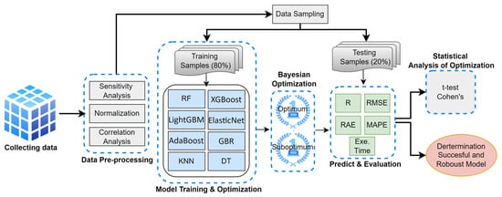
Figure 1.
The flowchart of the study.
The dataset used in the study was compiled from 45 articles [27,28,29,30,31,32,33,34,35,36,37,38,39,40,41,42,43,44,45,46,47,48,49,50,51,52,53,54,55,56,57,58,59,60,61,62,63,64,65,66,67,68,69,70,71] in the literature. In the pre-processing stage, the input variables in the dataset were first visualized using Violin Plots to examine their distributions. The graphical analysis revealed that the data did not exhibit a normal distribution, which was then evaluated using the Shapiro–Wilk test. Since the statistical test results confirmed that the dataset was not normally distributed, it was normalized using the standard scaling technique. Finally, the importance levels of the dataset’s features were analyzed using the Sensitivity Analysis technique.
Eight machine learning models were trained using 80% of the dataset during the training phase, while the remaining 20% of the data was reserved for testing. The parameters of all models were optimized using Bayesian optimization. The selection of the best-performing model was based on the hyperparameter combinations that maximized the R value. To identify the most robust model, those capable of achieving high accuracy under suboptimal conditions—specifically, those with the highest minimum R values even under adverse conditions—were preferred. This approach allowed for assessing a model’s robustness by considering not only its optimal (best-case) performance but also its performance under suboptimal (worst-case) conditions.
After the training process, the prediction performance of the models on the test set was evaluated using the metrics R, Root Mean Squared Error (RMSE), Relative Absolute Error (RAE), Mean Absolute Percentage Error (MAPE), and execution time. Comparisons based on these performance metrics identified the most accurate and robust model. Furthermore, the prediction performances of the models under optimal and suboptimal conditions were analyzed using a t-test, while the magnitude of the differences was assessed with Cohen’s d metric.
2.1. Dataset Description
This study utilized reliable empirical data (including laboratory and pilot plant experimental data) from the literature. The data were collected from 45 articles [27,28,29,30,31,32,33,34,35,36,37,38,39,40,41,42,43,44,45,46,47,48,49,50,51,52,53,54,55,56,57,58,59,60,61,62,63,64,65,66,67,68,69,70,71] published in databases such as Google Scholar, Scopus, and Web of Science. Since this study aims to identify the most reliable and robust machine learning model for predicting CO, CO2, H2, and CH4, only studies without missing values for these output variables were selected. The dataset used in the study consists of 12 input variables and four output variables obtained through the biomass gasification method. The statistical information is provided in Table 2.
Table 2.
Descriptive data statistics.
2.2. Pre-Processing Step
Data pre-processing is a critical step to ensuring the quality and reliability of machine learning models. The initial step in the pre-processing pipeline was outlier analysis. Outliers, which represent extreme deviations from the normal range of data, can adversely affect model performance and distort statistical properties. The Z-score method was applied to detect outliers, with a threshold of z > 3 used for identification. Z-score is a statistical technique that measures how many standard deviations a data point is from the mean. The absolute value of the Z-score indicates how “normal” or “outlier” a data point is within the dataset [72]. The Z-score was calculated for each data point using Equation (1).
where denotes a data point, μ is the mean, and σ is the standard deviation of the corresponding feature.
The proportion of outlier samples in the datasets used in this study was less than 10%; therefore, these samples were removed to ensure a more representative and consistent dataset for modeling.
Following outlier detection, normalization was performed to enhance the performance of machine learning algorithms. All features needed to be on the same scale to ensure more accurate results. Normalization was applied to constrain the data within a specific range (typically [0, 1] or [−1, 1]). This is especially important for distance-based algorithms, as such algorithms may produce erroneous results when dealing with features on different scales. Moreover, ensuring features have similar scales can facilitate faster learning and help mitigate model biases. In particular, when the data follow a normal distribution, model performance tends to be more stable [73]. In this study, the distributions of the variables in the dataset are illustrated using Violin Plots in Figure 2A. The distributions of the variables after normalization using standard scaling are shown in Figure 2B.
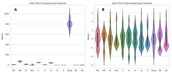
Figure 2.
Violin Plots of the original dataset (A) and the normalized dataset (B).
As shown in the Violin Plots (Figure 2A), significant scale differences and irregularities exist among the variables in the original dataset. In particular, the temperature variable exhibits a wide range of values (ranging from 600 to 1100). In contrast, all other variables are distributed within narrower ranges, with the highest value being 83. This results in the temperature variable suppressing the effect of the other variables, leading to pronounced heterogeneity in the dataset. Such disparities can complicate the learning process in machine learning models, as the models may overemphasize variables with larger values while disregarding the contributions of other variables. Therefore, applying preprocessing techniques such as normalization or standardization is critical to eliminating the biases caused by large-scale differences. These methods ensure all variables are brought to similar scales, contributing to more balanced and effective model performance.
The normality assumption of the dataset was assessed using the Shapiro–Wilk test. The results of the test indicated that the normality assumption could be rejected for all variables (Table 3). The p-values for all variables were below 0.05, suggesting a significant deviation from normal distribution. Notably, the low Shapiro–Wilk statistic values clearly illustrate the extent of this deviation. This deviation from normality may require additional procedures, such as normalization or transformation during the data analysis and modeling stages. Such statistical tests are crucial for understanding the characteristics of the data and ensuring more accurate results in the modeling phase.
Table 3.
Shapiro–Wilk test results.
The results of the Shapiro–Wilk test, presented in Table 3, indicate that none of the variables are normally distributed. The p-values for all variables are below 0.05, suggesting a significant deviation from normal distribution. These findings confirm that the dataset has a non-normally distributed structure and support the need for applying techniques such as normalization or transformation during the data preprocessing phase.
Sensitivity analysis (SA) is a highly popular feature selection method to highlight important features in a dataset [74]. It is performed to understand the overall effect of input variables on the model’s output and to assess which variables have the potential to influence this output [74]. The formulas in Equations (2) and (3) were used to calculate the contribution of each variable to the predicted output [75,76,77].
Here, fmax(xi) and fmin(xi) represent the maximum and minimum values of the ith prediction model output, respectively. The input values are held constant at their mean values. Ni provides the range of the ith input variable by calculating the difference between fmax(xi) and fmin(xi).
The contribution of each input parameter to the predicted output for CO was measured using sensitivity analysis, and the results for both the original and normalized datasets are presented in Figure 3.
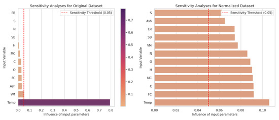
Figure 3.
Influence of input parameters on the prediction of CO levels for the original and normalized dataset.
Figure 3 compares the model’s sensitivity to the inputs for both the original and normalized datasets. In the original dataset, the Temp (temperature) variable was identified as the most dominant parameter by far, and it was observed that the model was overly dependent on this variable. This issue arose from the uneven distribution of the data, which leads to limited effects from the other variables. For example, variables such as N, MC, and VM were found to have a sensitivity threshold below 0.05 and showed no significant impact on the model.
When the dataset was normalized, the effects of all variables on the model were more evenly distributed. Variables such as N, SB, and MC showed the highest sensitivity, while Ash, ER, and VM exhibited the lowest sensitivity. However, even low-impact variables became more significant thanks to the normalization of the data. This demonstrates that normalization helps provide a fairer analysis by equalizing the effects of variables with different scales.
Our study emphasizes the impact of normalization on sensitivity analysis. Although the Temp variable appeared to be the most important feature in the original dataset, the Sulfur (S) variable exhibited the highest sensitivity in the normalized dataset. These results show that normalization reduces model bias, accurately reflecting the features’ relative effects. Therefore, the normalization step is crucial for enhancing model accuracy and the reliability of the analysis results.
2.3. Machine Learning Methods
In this study, eight different machine learning models were used to predict biomass gasification gases. The reason for selecting these models is to determine the most successful method for gas composition prediction by comparing their modeling performances in both linear and nonlinear structures. Additionally, the diversity of the models used allows for examining their capacity to adapt to different data characteristics.
Random Forest (RF) Regressor is an ensemble learning model that builds multiple decision trees and combines their results to make more accurate predictions [78]. Each tree is trained on a random subset of the data, and the final prediction is made by aggregating the votes of all trees. This method improves generalization capacity while reducing the risk of overfitting and is particularly effective with large datasets. RF ensures high accuracy for input features and is particularly successful in capturing complex, nonlinear relationships. In this study, the model was implemented using the RandomForestRegressor function in Python.
Extreme Gradient Boosting (XGBoost) is an optimized version of the gradient boosting algorithm, offering a high-performance and efficient learning process. XGBoost works by minimizing the error rates of previous trees with each new tree, with each iteration enhancing the model’s accuracy. This method is known for fast learning processes, high accuracy, and regularization techniques. XGBoost’s success is driven by optimization methods such as regularization and early stopping, which prevent overfitting. Moreover, it operates efficiently with large datasets and complex relationships, minimizing computational time. XGBoost’s parallel processing capability makes it especially fast and effective for large datasets. With its high accuracy, speed, and regularization advantages, this model is widely popular for classification and regression problems. The model was implemented using the XGBRegressor function.
Light Gradient-Boosting Machine (LightGBM) is an alternative to XGBoost and is specifically designed to work faster and more efficiently with large datasets and high-dimensional features. LightGBM uses a histogram-based learning approach, which leads to faster results with lower memory consumption. This study implemented the model using the LGBMRegressor function in Python.
Elastic Net is a regression model that combines the Lasso (L1) and Ridge (L2) regularization methods. While Lasso encourages feature selection, Ridge provides greater regularization (shrinkage). Elastic Net combines the benefits of both methods, improving performance with high-dimensional datasets, and is especially effective in cases of multicollinearity (highly correlated features). In this study, the model was developed using the ElasticNet function.
Adaptive Boosting (AdaBoost) constructs a strong model using a series of weak learners, typically decision trees. Each iteration aims to correct the errors of the previous model to form a more accurate one. AdaBoost takes advantage of combining multiple weak classifiers to achieve high accuracy and strengthens simple models that may tend to overfit. This model was implemented in Python using the AdaBoostRegressor function.
Gradient-Boosting Regressor (GBR) implements the basic gradient boosting algorithm, which builds a strong model from weak learners. This algorithm iteratively creates a new model to correct the errors of the previous one, aiming to minimize errors and increase accuracy with each step. GBR typically requires more computational power and time, as each iteration focuses on correcting the errors from the previous model, which increases computational costs. GBR can learn nonlinear and complex relationships, but it can be prone to overfitting without regularization. However, with the right hyperparameter optimization, GBR can provide high accuracy and strong generalization capabilities. This method performs well, especially with fewer trees, and maintains model interpretability. The model was implemented using the GradientBoostingRegressor function in Python.
K-Nearest Neighbors (KNN) is an algorithm that predicts a new data point based on the nearest kk neighbors in the dataset. KNN typically employs distance metrics, such as Euclidean distance, to identify the closest neighbors. This approach is particularly effective for capturing nonlinear relationships and is widely recognized for its intuitive structure [79]. However, its computational cost can be significant for large datasets, as each prediction requires comparisons with the entire dataset. KNN performs well when the data distribution is homogeneous and exhibits nonlinear patterns. Key parameters for this model include k (the number of neighbors) and the distance metric. The model was implemented in Python using the KNeighborsRegressor function.
A Decision Tree (DT) transforms data into a tree structure, making decisions for each data point. Trees classify or perform regression on data points based on their features. Decision trees increase model interpretability because each decision is based on a specific feature of the data, and this structure can be visualized. However, excessively deep trees may lead to overfitting, so techniques like pruning are used to limit model complexity. Decision trees can learn nonlinear and complex relationships, but overly deep trees can reduce generalization capability [80]. The model’s performance can be optimized using hyperparameters such as max_depth and min_samples_split. In this study, the model was implemented using the DecisionTreeRegressor function in Python.
2.4. Hyperparameter Optimization
Model hyperparameters are critical factors that directly influence the behavior and performance of machine learning models. The process of hyperparameter tuning plays a significant role in determining the success of a model. However, many studies in the literature have typically relied on the default parameter values of machine learning methods, with limited in-depth investigation into the effects of hyperparameter tuning on model performance. This study employs Bayesian optimization to determine the optimal model parameters. Bayesian optimization facilitates a more efficient search process by considering the results of previous trials, thereby enabling the identification of the best hyperparameter combinations. This method allows for more accurate results with fewer trials, making the optimization process more efficient. Additionally, narrowing the search space aims to reach the optimal solution more quickly. This approach has proved to be highly effective in enhancing the model’s overall performance and reducing computational costs.
In contrast, traditional methods such as manual search, grid search, and random search are commonly used. However, these methods can be computationally expensive and time-consuming when applied to models with many hyperparameters or when evaluating each hyperparameter set, which is costly. Bayesian optimization, on the other hand, offers a more efficient alternative by directing the search process through probabilistic models. This method bases the model’s performance on a probabilistic function and iteratively improves the search space, allowing for the determination of optimal hyperparameters with fewer evaluations. As a result, the computational burden is reduced and the hyperparameter tuning process is expedited, making Bayesian optimization a preferred option, especially for complex and high-dimensional machine learning problems [81]. The optimization process follows these steps:
- Selection of Initial Points: Several random combinations of parameters are initially selected.
- Model Training: The model is trained with the selected hyperparameters, and predictions are made on the test data.
- Acquisition Function Maximization: The acquisition function selects new hyperparameters.
- Iteration: These steps are repeated until the optimal set of parameters is found.
In this study, hyperparameter optimization was conducted with two objectives. The first objective was to identify the most successful predictive model by determining the optimal combinations of hyperparameters yielding the highest R values under ideal conditions. The second objective was to identify the hyperparameter combinations in suboptimal conditions, where the models exhibit the poorest predictive performance, and to ensure that the model still achieves high accuracy in this scenario. In this way, the model’s performance was tested for high accuracy, consistency, and stability in its results.
The BayesianOptimization function was used in the Python environment to develop this model, with default parameters applied for the acquisition function and kernel type. The parameters used for the models, the ranges of tested parameter values, and the hyperparameters determined for both optimal and suboptimal conditions are presented in Table 4. The parameter ranges of the models were kept broad to reduce the risk of overfitting and achieve more robust results. Broad parameter ranges allow the model to be effectively tested with diverse parameter combinations, thereby contributing to the most accurate results.
Table 4.
Model hyperparameters defined for the prediction system.
2.5. Model Performance Evaluation
Various metrics were used to evaluate the performance of ML prediction models. The correlation coefficient is a key measure that indicates how close the model’s predictions are to the actual data, with high values expected in strong linear relationships. RMSE calculates the model’s prediction errors, showing how accurate the model’s predictions are. The lower this value is, the higher the accuracy of the model. RAE evaluates the model’s predictions in relation to the average error rate of the dataset. MAPE measures the percentage error between the predicted and actual values, providing insight into the relative accuracy of the model, especially for datasets with varying scales. Additionally, execution time measures the total time spent by the model while making predictions, an important parameter for efficiency, as faster processing times enhance the model’s applicability in large datasets. Each of these metrics is critical to understanding the model’s accuracy, efficiency, and generalization ability.
We conducted t-tests to evaluate whether the differences in the R values between optimal and suboptimal conditions were statistically significant. Specifically, the means of the R values under optimal conditions were compared to those under suboptimal conditions for each model. The t-test formula was applied as follows in Equation (4):
where and are the means of the two groups, and are their respective variances, and and are the sample sizes of the two groups.
Cohen’s d was used to measure the effect size of the differences observed in the R values between optimal and suboptimal conditions, using the formula in Equation (5).
3. Results
CO, CO2, H2, and CH4 gases are significant outputs in biomass gasification processes. These four gases are produced during the decomposition of biomass in the gasification process and play a critical role in energy production and environmental impacts. This section separately examines the prediction performance of different machine learning methods for CO, CO2, H2, and CH4 gases under optimal and suboptimal conditions.
3.1. Prediction of Carbon Monoxide (CO) Gas Levels
CO is a toxic gas produced in environments where combustion processes occur with insufficient oxygen. It is released during the decomposition of biomass in gasification and holds significance as a fuel due to its high energy content. Accurate prediction of CO levels is a critical step in optimizing the efficiency of the gasification process. Maintaining CO levels within a specific range is essential for efficient gasification, as CO can also indicate energy.
The correlation matrix in Figure 4 illustrates the linear and nonlinear relationship between CO and input variables in the gasification process. This matrix is presented as a heatmap to visualize the relationships between variables, with color intensity representing the correlations’ strength and direction. Insights derived from the relation help us understand the interactions between variables and serve as a starting point for gas level prediction using machine learning models.

Figure 4.
Linear and nonlinear relationships between CO output and input variables.
When the linear correlation matrix was examined (Figure 4), the variables most strongly related to CO output were found to be H (0.33), VM (0.32), and SB (0.30). These results indicate that these variables have a moderate positive impact on CO output. Increases in H, VM, and SB were observed to raise CO output; however, these effects were similar in magnitude, suggesting that other factors, which might provide stronger relationships, should be considered to fully explain CO output. On the other hand, the high negative correlation (−0.96) observed between carbon (C) and oxygen (O) highlights the importance of the chemical balance between these two elements. Similarly, the strong negative relationship (−0.80) between Ash and VM suggests that a reduction in volatile components during combustion leads to an increase in ash content.
In the analysis of nonlinear relationships, the variables most strongly related to CO output were identified as C (0.34), SB (0.32), and FC (0.28). This analysis, in particular, shows that the C variable has the highest nonlinear impact on CO output, with differences in its value potentially causing significant changes in CO output. While SB and FC exhibited meaningful effects, with mutual information values of 0.32 and 0.28, respectively, their relationship with CO output was not as strong as that of C. These results indicate that both linear and nonlinear methods are necessary to accurately model the effects of variables on CO output. Table 5 presents a comparative analysis of the test performances of eight machine learning models in predicting CO under optimal and suboptimal conditions.
Table 5.
Test performances of CO level prediction under optimal and suboptimal conditions.
When examining the best results obtained for CO level prediction by the models, it was observed that the XGBoost (RMSE = 3.109, RAE = 7.003, MAPE = 7.44) and GBR (RMSE = 3.174, RAE = 7.142, MAPE = 7.334) models exhibited the lowest errors. These results indicate that both models provide accurate predictions with low error rates; however, the XGBoost model outperforms the others. In contrast, the Elastic Net and KNN models demonstrate limited predictive performance with high error rates.
When examining the models’ prediction performances under suboptimal conditions, the XGBoost model provided CO level predictions with lower error (RMSE = 5.291, RAE = 12.804, MAPE = 14.286) compared to the other models. Furthermore, it was observed that XGBoost still offered high accuracy (R = 0.889) under these conditions. The Elastic Net and KNN models performed inadequately, exhibiting high error and low R values (R = 0.324 and R = 0.289, respectively). These results demonstrate that the XGBoost model achieved successful CO level predictions under challenging conditions.
The difference in prediction performance between the models under optimal and suboptimal conditions was evaluated using a t-test, and it was found that the difference was statistically significant (t-statistic = 5.03, p-value = 0.0015). Cohen’s d value (1.7788) indicates that hyperparameter optimization substantially impacts model performance. This analysis reveals that different parameters are crucial to model accuracy, and the performance gap is distinctly noticeable.
3.2. Prediction of Carbon Dioxide (CO2) Gas Levels
CO2 is a stable compound that forms during the gasification of biomass. Although its energy content is lower than CO and H2, it is an important indicator providing valuable insights into the process. The prediction of CO2 levels is critical for assessing environmental impacts and achieving low-emission targets in sustainable energy production efforts. Furthermore, CO2 concentrations are a key parameter affecting the efficiency of the gasification process. The relationship between CO2 and the input variables of the gasification process is examined in the correlation matrix presented in Figure 5.
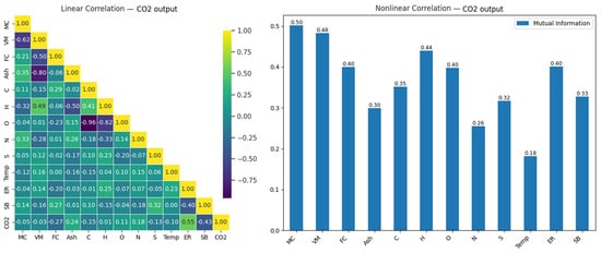
Figure 5.
Linear and nonlinear relationships between CO2 output and input variables.
A strong positive linear correlation (0.55) was observed between CO2 output and the ER variable. This relationship indicates a direct connection between these two variables in energy conversion processes, with higher energy demands being associated with increased CO2 emissions. In contrast, a strong negative relationship (−0.43) was found between CO2 and SB. This can be attributed to changes in process stability or the equilibrium processes occurring during combustion. A weak negative relationship (−0.27) was observed between CO2 and FC, which suggests the presence of a latent interaction that may be better explained through nonlinear analysis. On the other hand, the strong negative correlation (−0.96) observed between C and O explains the chemical equilibrium processes between carbon and oxygen. Similarly, a strong negative correlation (−0.80) was found between Ash and VM, reflecting processes such as the increase in ash content due to a decrease in volatile components during combustion.
In the nonlinear analysis, the variables MC (0.56), VM (0.51), and FC (0.56) were found to be determinants of CO2 output, according to their mutual information values. This highlights the effect of fuel moisture content and volatile component ratios on CH4 formation. In contrast, variables such as SB (0.19), ER (0.22), and Temp (0.22) exhibited a limited effect with lower values. The increased importance of O and N in the nonlinear analysis, despite being seen as having low impacts in the linear analysis, suggests that oxygen and nitrogen play an indirect but significant role in chemical reaction processes.
In conclusion, nonlinear methods are more effective in detecting complex and indirect relationships. These results demonstrate the critical importance of using nonlinear analysis methods in modeling processes. Table 6 presents the prediction performance of machine learning models for CO2 gas levels under optimal and suboptimal conditions.
Table 6.
Test performances of CO2 prediction under optimal and suboptimal conditions.
When examining the performances of models under optimal conditions for CO2 level prediction, the XGBoost model (RMSE = 3.590, RAE = 8.667, MAPE = 11.616) achieved the best results, closely followed by the GBR model (RMSE = 3.599, RAE = 9.282, MAPE = 11.606). In contrast, the Elastic Net model exhibited the highest error rates, demonstrating significantly lower performance than the other models, with RMSE = 8.911, RAE = 24.923, and MAPE = 43.798.
Under suboptimal conditions, the XGBoost model outperformed the other models in CO2 level prediction, with RMSE = 6.432, RAE = 17.752, and MAPE = 28.253. This finding reveals that XGBoost can make effective predictions even under harsh conditions. On the other hand, the KNN model shows a significant increase in prediction error.
Statistical analyses revealed hyperparameter changes significantly impacted model prediction performance (t-statistic = 4.94, p-value = 0.0017). Cohen’s d value (1.7451) indicates that hyperparameter optimization strongly affected model performance. These results highlight the critical importance of selecting the correct hyperparameters to improve the accuracy of CO2 level predictions.
3.3. Prediction of Hydrogen (H2) Gas Levels
H2 is a high-energy-content and environmentally friendly gas. Hydrogen produced during gasification is an important fuel, particularly among renewable energy sources. The prediction of H2 levels is critical for enhancing energy efficiency and obtaining sustainable fuel. Estimating hydrogen content is crucial in optimizing biomass gasification, as higher hydrogen content leads to higher energy production. The relationship between H2 and the input variables in the gasification process is examined in the correlation matrix presented in Figure 6.

Figure 6.
Linear and nonlinear relationships between H2 output and input variables.
When Figure 6 is examined, a strong positive relationship (0.61) between H2 and SB is observed, while a strong negative relationship (−0.60) exists between ER and H2. Additionally, a very strong negative correlation (−0.96) is observed between C and O, and a significant negative relationship (−0.80) is seen between Ash and VM. These strong negative relationships provide important insights into how these variables may influence each other during the modeling process.
In the nonlinear analysis, the highest mutual information (MI) values for H2 output were observed in the MC (0.77), VM (0.78), FC (0.78), and Ash (0.78) variables. This indicates that these variables make significant contributions to H2 production. Furthermore, many variables that showed low effects in the linear correlation were found to be more prominent in the nonlinear analysis. This suggests that nonlinear analyses provide a broader perspective compared to linear methods, offering a better evaluation of the relationships between variables.
Table 7 presents the prediction performances for H2 gas levels under optimal and suboptimal conditions.
Table 7.
Test performances of H2 level prediction under optimal and suboptimal conditions.
The H2 level prediction results under optimal conditions demonstrate that the XGBoost model achieves excellent prediction accuracy (RMSE = 2.774, RAE = 6.471, MAPE = 7.542). Although the execution time of the XGBoost model is slightly higher than that of other models, it is approximately 37 s, which can be considered a negligible delay.
When considering the models’ lowest performances in H2 level prediction, the XGBoost model (RMSE = 5.707, RAE = 13.280, MAPE = 16.290) stands out, with relatively low error rates compared to the others. This highlights XGBoost’s flexibility in learning both linear and nonlinear relationships. Following XGBoost is the GBR model, while the poorest prediction performance is observed in the KNN model (RMSE = 13.323, RAE = 33.220, MAPE = 42.218). This suggests that linear models provide lower accuracy in H2 level prediction.
The results of the t-test analysis (t-statistic = 3.13, p-value = 0.0166) reveal a statistically significant difference in the models’ optimal and suboptimal prediction performance (p < 0.05). Moreover, Cohen’s d value (1.1067) confirms the strong effect of hyperparameter tuning on model performance.
3.4. Prediction of Methane (CH4) Gas Levels
CH4 is another energy-rich gas produced during the gasification process. As the primary component of natural gas, CH4 has the potential to provide energy during the combustion of biomass. The prediction of CH4 levels is essential for assessing the energy efficiency of the process and optimizing its use as a fuel. Specifically, the amount of methane used as an energy source in the biomass gasification process significantly affects the system’s overall performance. The relationship between CH4 and the input variables in the gasification process is examined in the correlation matrix presented in Figure 7.
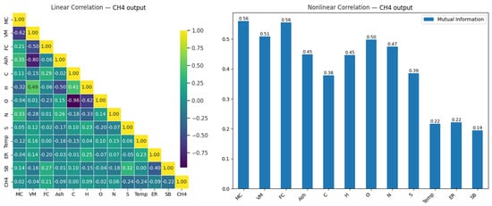
Figure 7.
Linear and nonlinear relationships between CH4 output and input variables.
As seen in Figure 7, the relationships between the input variables and the CH4 output are generally weak, with the input variables showing the highest correlation being SB (0.23), FC (0.20), S (−0.21), and Temp (−0.21). This indicates that predicting CH4 output with linear models may provide limited success. However, other noteworthy relationships between the variables may offer potential information for different analysis methods or modeling approaches. For example, a strong negative correlation (−0.77) is observed between Ash and VM, and an even stronger negative relationship (−0.93) is observed between C and O. This suggests strong negative relationships between these variables. Such relationships may help better understand the effects of the variables during modeling.
In the analysis of nonlinear relationships, the variables MC (0.50), VM (0.51), and FC (0.56) show the highest mutual information values for the CH4 output. This indicates that these variables contribute significantly to CH4 production. In contrast, variables such as SB (0.19), ER (0.22), and Temp (0.22) show weaker effects, with lower values. Moreover, it is noteworthy that the O and N variables, which appear to have low impacts in the linear analysis, become more significant in the nonlinear analysis. This demonstrates that nonlinear approaches can reveal deeper relationships and should be considered in modeling processes.
As a result, it appears difficult to strongly predict CH4 based on a linear model; thus, advanced modeling techniques, such as machine learning models, which can address the interactions between different properties, are more appropriate. CH4 gas has been predicted using ML models, and the prediction performance results under optimal and suboptimal conditions are presented in Table 8.
Table 8.
Test performances of CH4 level prediction under optimal and suboptimal conditions.
The optimal performance of the models for CH4 level prediction revealed that the XGBoost model achieved the lowest error rates (RMSE = 1.040, RAE = 10.547, MAPE = 14.338). XGBoost was followed by GBR and LightGBM models in terms of performance. Regarding execution time, XGBoost demonstrated a balanced performance between speed and accuracy, making predictions in only 52 s. The results presented in Table 8 highlight the effectiveness of XGBoost for CH4 level prediction, with its ability to learn complex data relationships leading to highly accurate predictions. Despite the weak correlations between CH4 output and input variables, as shown in Figure 7, XGBoost successfully navigated these challenges and delivered strong results. XGBoost facilitates the modeling of more complex data structures through tree-based architectures. Due to the learning capability of XGBoost, high prediction accuracy is achieved even in cases of nonlinear relationships or variables with low correlations.
Suboptimal conditions also revealed XGBoost’s superior performance (RMSE = 1.591, RAE = 13.750, MAPE = 16.411) compared to other models. In contrast, the Elastic Net and DT models produced predictions with the lowest accuracy, demonstrating weak performance. Even in the worst-case scenario, XGBoost achieved a correlation value of 0.837, highlighting the model’s flexibility and robustness.
The t-statistic of 5.44 and p-value of 0.0010 indicate a statistically significant difference between the models’ optimal and suboptimal prediction performances (p < 0.05). This finding underscores the critical role of hyperparameter optimization in enhancing model performance. Additionally, the high Cohen’s d value of 1.9227 emphasizes the significant impact of hyperparameter optimization on model success.
4. Discussion
Biomass gasification is critical for renewable energy production and reducing greenhouse gas emissions. Accurate prediction of gas composition during this process supports environmental sustainability by improving energy efficiency. The prediction of CO, CO2, H2, and CH4 gas levels in the biomass gasification process using machine learning methods facilitates the management of complex processes, enabling rapid and accurate predictions. Specifically, in systems like biomass gasification processes that involve numerous variables, predicting the levels of these four major gases offers the following advantages:
- Accurate predictions of gas levels through machine learning optimize the ratios of gases to be used as fuel, thereby enhancing energy efficiency. This ensures that the biomass gasification process operates in a more efficient and energy-saving manner.
- The accurate prediction of CO, CO2, H2, and CH4 levels allows for developing environmentally friendly strategies to reduce their emissions. This, in turn, enhances the environmental sustainability of biomass gasification processes.
- Machine learning models allow for rapidly predicting gas levels in biomass gasification processes. This contributes to the process’s time efficiency and enables operators to make faster decisions.
- Instead of relying on prolonged experimental testing, machine learning allows for rapid and accurate predictions, thereby increasing the cost-effectiveness of the processes and providing significant time savings.
This study conducted analyses to determine the most successful and robust model for predicting the levels of four gases: CO, CO2, H2, and CH4. However, depending on specific needs, each gas can be predicted individually. For example, if researchers are focused on sustainable energy production, particular attention may be given to H2, as it is often one of the most critical components. In studies related to biogas production, CH4 output will emerge as an important parameter. If the focus is on environmental impacts, the carbon cycle, or carbon capture studies, the prediction of CO2 levels may become a priority. While less emphasized than the other gases, CO remains an important component in combustion or reforming processes.
The aim was to identify the most successful and robust ML models for predicting levels of the gases CO, CO2, H2, and CH4 generated during biomass gasification. Bayesian optimization was used to determine the models’ hyperparameters under optimal and suboptimal conditions. In the optimal case, parameter combinations leading to the highest R values were selected, while in the suboptimal case, those corresponding to the lowest R values were chosen. The goal was to predict gas levels under both optimal and suboptimal conditions accurately. This approach ensured that the selected models performed well and provided consistent results under suboptimal conditions, making them more reliable in real-world applications.
The prediction performance of the models was also visualized and analyzed using a Taylor diagram. In the Taylor diagram, the Correlation Coefficient Contours (Arcs) represent the relationships between the observed values and the model predictions. A correlation coefficient approaching 1 indicates high prediction accuracy, while the radius (standard deviation) describes the variations in the models’ predictions. Standard deviation values closer to those of the observed data signal more successful models.
In the prediction of CO levels, the performances of the models under optimal and suboptimal conditions, based on hyperparameter combinations, are presented comparatively in the Taylor diagram in Figure 8. Upon examining the Taylor diagram, it can be observed that the XGBoost model has a correlation coefficient of 0.951 and a standard deviation (8.51) that aligns closely with the observed data. When comparing the suboptimal prediction performances of the models, it was found that the XGBoost model exhibits the highest correlation coefficient (0.889) and the lowest RMSE value (5.291). In contrast, the KNN model significantly differs between its optimal (R = 0.910) and suboptimal (R = 0.289) performance. This is due to the KNN model’s performance varying significantly depending on the sensitivity of its hyperparameter settings and the number of neighbors. The KNN model can yield different results depending on the data density and convergence rate, which causes fluctuations in its performance. Additionally, if the number of neighbors is not correctly determined in high-dimensional data, KNN can lead to issues such as overfitting or underfitting. Therefore, the difference between the optimal and suboptimal prediction performances of the KNN model reflects the model’s sensitivity to hyperparameter selection. This suggests that the model’s robustness is limited due to performance fluctuations with different parameters. On the other hand, the XGBoost model demonstrates strong performance even in the suboptimal scenario, indicating its robustness. This highlights the consistently high accuracy the XGBoost model provides, even when faced with challenges. The model’s flexibility allows for reliable results, even in real-world applications with more prevalent uncertainty and data variability.
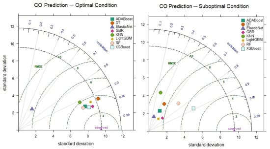
Figure 8.
Taylor diagram of CO level prediction performance for optimal and suboptimal conditions.
When examining the optimal CO2 level prediction results of the models (Figure 9), the XGBoost model stands out as the most successful, with a correlation coefficient of 0.954 and a standard deviation value of 11.06. The fact that the XGBoost model still achieves a correlation coefficient of 0.858 and an RMSE value of 6.463 in the suboptimal condition further indicates its superior performance. On the other hand, the KNN model, with a maximum correlation of 0.934 and a minimum of 0.175 in CO2 level prediction, demonstrates unreliable and inconsistent performance under poor conditions.
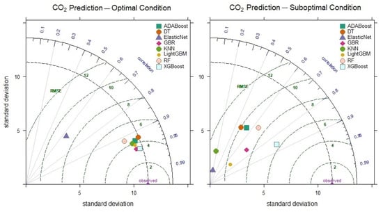
Figure 9.
Taylor diagram of CO2 level prediction performance for optimal and suboptimal conditions.
When comparing the prediction performances of the models for H2, it is observed that under optimal conditions, the XGBoost model achieves the highest R value of 0.981 (Figure 10). Similarly, under suboptimal conditions, the XGBoost model outperforms the other models, reaching an R value of 0.941. These findings demonstrate that the XGBoost model offers more robust performance, achieving higher accuracy and more consistent prediction variations than other models, even under suboptimal conditions. The KNN model reached an optimal R value of 0.979, and the 0.316 decrease in performance under suboptimal conditions indicates the model’s sensitivity to parameter optimization.
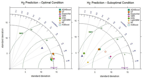
Figure 10.
Taylor diagram of H2 level prediction performance under optimal and suboptimal conditions.
The weak relationships in the correlation matrix between the CH4 outputs and inputs shown in Figure 7 indicate that the linear dependencies in the data are low. However, machine learning models have successfully learned complex and nonlinear relationships, demonstrating excellent prediction performance. The XGBoost model, with parameter optimization, achieved the highest prediction performance, reaching a correlation coefficient of 0.933 (Figure 11). As seen in Figure 11, even under suboptimal conditions, it outperformed other models with a correlation of 0.856 and an RMSE value of 1.503. These results indicate that the XGBoost model can make CH4 level predictions successfully and consistently. On the other hand, the prediction performances of the Elastic Net, KNN and DT models significantly decreased under suboptimal conditions, demonstrating that these models have limited capacity to learn nonlinear relationships.
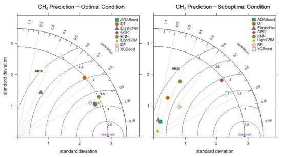
Figure 11.
Taylor diagram of CH4 level prediction performance under optimal and suboptimal conditions.
The findings of this study demonstrate that machine learning models, particularly the prediction system developed using XGBoost, can predict CO, CO2, H2, and CH4 gas levels in biomass gasification processes with high accuracy and consistency. Bayesian optimization has enhanced accuracy and enabled the acquisition of resilient predictions by optimizing the model parameters. The XGBoost model has outperformed other models in accuracy and robustness. Notably, the superior performance of the XGBoost model under suboptimal conditions cannot be attributed to model regularization or parameter optimization, as both optimal and suboptimal conditions were tested using the same set of parameters. The model’s ability to maintain high performance, even under suboptimal conditions, can be attributed to XGBoost’s inherent robustness, capacity to handle noisy or incomplete data effectively, and ability to capture complex, suboptimal relationships.
However, their low robustness has marked the Elastic Net, KNN, and DT models. These models exhibited significant performance differences under optimal and suboptimal conditions, indicating their limited generalization capacity and the substantial impact of parameter optimization on performance. Elastic Net failed to deliver the expected accuracy in biomass gasification processes, where complex and nonlinear relationships dominate. The KNN model, due to its requirement to use the entire dataset for each prediction, resulted in increased computation time for large datasets, leading to a loss of accuracy. Decision Trees, on the other hand, performed poorly on new data outside the training set, due to over-branching and overfitting issues. These challenges limit the applicability of these models in complex and nonlinear processes.
The advantages of this study include the development of ML models with different architectures for predicting biomass gas levels and the public sharing of the Python source code. This enables researchers to replicate similar studies and enhance existing models. Furthermore, the prediction performances of the models were tested not only under optimal conditions but also in suboptimal conditions. In this way, the models’ abilities to make successful predictions and their robustness were assessed. This approach aids in selecting models capable of making accurate predictions even in worst-case scenarios with real-world data. Finally, it was observed that there are few studies focused on hyperparameter optimization in the literature. This study tested models with different parameters and broad parameter ranges, enhancing their flexibility. As a result, models that are not only optimized with specific parameters but also adaptable to varying conditions, and thus more robust and reliable, were obtained.
Despite the clear advantages of the study, some limitations exist. Studies on biomass gasification processes, like the one presented here, often face challenges due to the small size of datasets. While data were collected from 45 different literature sources, the dataset in this study contains only 413 samples. The small size of the dataset may negatively affect model accuracy and generalization capability, as models based on larger and more diverse datasets are likely to yield more robust and reliable results. In this regard, producing more comprehensive datasets related to biomass gasification processes in laboratory settings and their public availability would significantly contribute to the literature in this field. Large datasets will enable the model to reduce data dependency and minimize the risks of overfitting, thereby facilitating the acquisition of more robust and generalizable results. Additionally, while hyperparameter optimization was performed, large datasets’ high computational time requirements may present practical challenges. Optimizing and testing each model can be time-consuming, and handling larger datasets becomes even more complex.
The findings of this study highlight the success and practical potential of the proposed machine learning model. The model can be applied to enhance operational efficiency in biomass gasification plants. Enabling dynamic management of the gasification processes facilitates the real-time optimization of these processes, offering a more efficient and flexible operational framework. The high accuracy of the model in predicting gas production and its components allows for more precise control of the processes, thereby improving operational efficiency and contributing to cost reduction. Thus, the proposed model can be a powerful tool for effectively managing processes in gasification plants.
5. Conclusions
This study evaluated eight ML models to predict the production of gases from biomass gasification (CO, CO2, H2, and CH4). The hyperparameter combinations for the optimal and suboptimal conditions of each model were determined using Bayesian optimization. The XGBoost model demonstrated superior performance and robustness in predicting the levels of all four gases separately, achieving the highest R values and the lowest error metrics in both optimal and suboptimal conditions. The findings highlight the potential of ML models in effectively predicting biomass gasification outputs, facilitating better process control, enhancing energy efficiency, and reducing environmental impact. Notably, the Bayesian optimization approach significantly improved the models’ accuracy and stability, particularly for XGBoost, which emerged as the most reliable model for capturing complex and nonlinear relationships. The Elastic Net and KNN models, on the other hand, not only exhibited the lowest R values under optimal conditions but also showed a significant decrease in performance under suboptimal conditions compared to the other models. These findings underscore the challenges of relying on models with limited robustness across varying parameter settings and emphasize the importance of careful model selection and parameter tuning. Future research could expand the dataset with a broader range of biomass feedstocks and integrate dynamic modeling techniques to account for temporal variations in gasification processes. Additionally, integrating ML models with real-time process control systems can further optimize biomass gasification for industrial applications.
Funding
This research received no funding.
Institutional Review Board Statement
Not applicable.
Informed Consent Statement
Not applicable.
Data Availability Statement
The raw data used in this manuscript are referenced in the literature section of the paper. The ML regression models developed in this study are available at https://github.com/pcihan/Biomass_gas_prediction.
Conflicts of Interest
The author declares no conflicts of interest.
Abbreviations
| AdaBoost | Adaptive Boosting |
| AFR | Air Fuel Ratio |
| BAG | Bagging |
| BFB | Bubbling Fluidized Bed |
| BFR | Biomass Feed Rate |
| BM | Bed Material |
| BLS-SVM | Binary Least Squares Support Vector Machine |
| C | Carbon |
| CCE | Carbon Conversion Efficiency |
| CFR | Coal Feed Rate |
| CGE | Cold Gas Efficiency |
| R | Correlation Coefficient |
| CU | Catalyst Usage |
| DT | Devolatilization Temperature |
| DTR | Decision Tree Regression |
| Elastic Net | Elastic Net |
| ER | Equivalence Ratio |
| FC | Fixed Carbon |
| GA | Gasifying Agent |
| GB | Gradient Boosting |
| GY | Gas Yield |
| GOP | Gasifier Operation Mode |
| GBR | Gradient-Boosting Regressor |
| GS | Gasifier Scale |
| H | Hydrogen |
| KNN | K-Nearest Neighbors |
| LARS | Least-Angle Regression |
| LightGBM | Light Gradient-Boosting Machine |
| LR | Linear Regression |
| LHV | Lower Heating Value |
| MAPE | Mean Absolute Percentage Error (MAPE) |
| MC | Moisture Content |
| MC-RF | Multi-Class Random Forest Classifiers |
| MW | Molecular Weight |
| MLP | Multilayer Perceptron |
| O | Oxygen |
| PS | Particle Size |
| PR | Polynomial Regression |
| RF | Random Forest |
| RAE | Relative Absolute Error |
| RR | Ridge Regression |
| RMSE | Root Mean Squared Error |
| RT | Reactor Type |
| SA | Sensitivity Analysis |
| SB | Steam Biomass Ratio |
| SCWG | Supercritical Water Gasification |
| SFR | Steam Flow Rate |
| SVR | Support Vector Regression |
| T | Time |
| Temp | Temperature |
| VM | Volatile Matter |
| W | Catalyst Loading Amount |
| X | Carbon Conversion |
| XGBoost | Extreme Gradient Boosting |
References
- Fang, Y.; Ma, L.; Yao, Z.; Li, W.; You, S. Process optimization of biomass gasification with a Monte Carlo approach and random forest algorithm. Energy Convers. Manag. 2022, 264, 115734. [Google Scholar] [CrossRef]
- Ismail, T.M.; Shi, M.; Xu, J.; Chen, X.; Wang, F.; El-Salam, M.A. Assessment of coal gasification in a pressurized fixed bed gasifier using an ASPEN plus and Euler–Euler model. Int. J. Coal Sci. Technol. 2020, 7, 516–535. [Google Scholar] [CrossRef]
- Ozbas, E.E.; Aksu, D.; Ongen, A.; Aydin, M.A.; Ozcan, H.K. Hydrogen production via biomass gasification, and modeling by supervised machine learning algorithms. Int. J. Hydrogen Energy 2019, 44, 17260–17268. [Google Scholar] [CrossRef]
- Nguyen, T.L.T.; Hermansen, J.E.; Nielsen, R.G. Environmental assessment of gasification technology for biomass conversion to energy in comparison with other alternatives: The case of wheat straw. J. Clean. Prod. 2013, 53, 138–148. [Google Scholar] [CrossRef]
- ASEAN. ASEAN Strategy on Sustainable Biomass Energy for Agriculture Communities and Rural Development in 2020–2030. 2019. Available online: https://www.fao.org/faolex/results/details/en/c/LEX-FAOC216870/ (accessed on 10 October 2024).
- Hossain, M.R.; Rana, M.J.; Saha, S.M.; Haseeb, M.; Islam, M.S.; Amin, M.R.; Hossain, M.E. Role of energy mix and eco-innovation in achieving environmental sustainability in the USA using the dynamic ARDL approach: Accounting the supply side of the ecosystem. Renew. Energy 2023, 215, 118925. [Google Scholar] [CrossRef]
- Alfarra, F.; Ozcan, H.K.; Cihan, P.; Ongen, A.; Guvenc, S.Y.; Ciner, M.N. Artificial intelligence methods for modeling gasification of waste biomass: A review. Environ. Monit. Assess. 2024, 196, 309. [Google Scholar] [CrossRef] [PubMed]
- Kushwah, A.; Reina, T.; Short, M. Modelling approaches for biomass gasifiers: A comprehensive overview. Sci. Total Environ. 2022, 834, 155243. [Google Scholar] [CrossRef]
- Li, J.; Yao, X.; Xu, K. A comprehensive model integrating BP neural network and RSM for the prediction and optimization of syngas quality. Biomass Bioenergy 2021, 155, 106278. [Google Scholar] [CrossRef]
- Devasahayam, S.; Albijanic, B. Predicting hydrogen production from co-gasification of biomass and plastics using tree based machine learning algorithms. Renew. Energy 2024, 222, 119883. [Google Scholar] [CrossRef]
- Sison, A.E.; Etchieson, S.A.; Güleç, F.; Epelle, E.I.; Okolie, J.A. Process modelling integrated with interpretable machine learning for predicting hydrogen and char yield during chemical looping gasification. J. Clean. Prod. 2023, 414, 137579. [Google Scholar] [CrossRef]
- Elmaz, F.; Yücel, Ö.; Mutlu, A.Y. Predictive modeling of biomass gasification with machine learning-based regression methods. Energy 2020, 191, 116541. [Google Scholar] [CrossRef]
- Mutlu, A.Y.; Yucel, O. An artificial intelligence based approach to predicting syngas composition for downdraft biomass gasification. Energy 2018, 165, 895–901. [Google Scholar] [CrossRef]
- Wen, H.-T.; Lu, J.-H.; Phuc, M.-X. Applying artificial intelligence to predict the composition of syngas using rice husks: A comparison of artificial neural networks and gradient boosting regression. Energies 2021, 14, 2932. [Google Scholar] [CrossRef]
- Yucel, O.; Aydin, E.S.; Sadikoglu, H. Comparison of the different artificial neural networks in prediction of biomass gasification products. Int. J. Energy Res. 2019, 43, 5992–6003. [Google Scholar] [CrossRef]
- Serrano, D.; Golpour, I.; Sánchez-Delgado, S. Predicting the effect of bed materials in bubbling fluidized bed gasification using artificial neural networks (ANNs) modeling approach. Fuel 2020, 266, 117021. [Google Scholar]
- Ozonoh, M.; Oboirien, B.; Higginson, A.; Daramola, M. Performance evaluation of gasification system efficiency using artificial neural network. Renew. Energy 2020, 145, 2253–2270. [Google Scholar] [CrossRef]
- Shahbaz, M.; Taqvi, S.A.; Loy, A.C.M.; Inayat, A.; Uddin, F.; Bokhari, A.; Naqvi, S.R. Artificial neural network approach for the steam gasification of palm oil waste using bottom ash and CaO. Renew. Energy 2019, 132, 243–254. [Google Scholar]
- Baruah, D.; Baruah, D.C.; Hazarika, M.K. Artificial neural network based modeling of biomass gasification in fixed bed downdraft gasifiers. Biomass Bioenergy 2017, 98, 264–271. [Google Scholar] [CrossRef]
- Zhao, S.; Li, J.; Chen, C.; Yan, B.; Tao, J.; Chen, G. Interpretable machine learning for predicting and evaluating hydrogen production via supercritical water gasification of biomass. J. Clean. Prod. 2021, 316, 128244. [Google Scholar] [CrossRef]
- Ascher, S.; Sloan, W.; Watson, I.; You, S. A comprehensive artificial neural network model for gasification process prediction. Appl. Energy 2022, 320, 119289. [Google Scholar]
- Li, W.; Song, Y. Artificial neural network model of catalytic coal gasification in fixed bed. J. Energy Inst. 2022, 105, 176–183. [Google Scholar] [CrossRef]
- Pandey, D.S.; Raza, H.; Bhattacharyya, S. Development of explainable AI-based predictive models for bubbling fluidised bed gasification process. Fuel 2023, 351, 128971. [Google Scholar] [CrossRef]
- Kargbo, H.O.; Zhang, J.; Phan, A.N. Robust modelling development for optimisation of hydrogen production from biomass gasification process using bootstrap aggregated neural network. Int. J. Hydrogen Energy 2023, 48, 10812–10828. [Google Scholar] [CrossRef]
- Elmaz, F.; Yücel, Ö.; Mutlu, A.Y. Evaluating the effect of blending ratio on the co-gasification of high ash coal and biomass in a fluidized bed gasifier using machine learning. Mugla J. Sci. Technol. 2019, 5, 1–12. [Google Scholar] [CrossRef]
- Ayub, H.M.U.; Rafiq, M.; Qyyum, M.A.; Rafiq, G.; Choi, G.S.; Lee, M. Prediction of process parameters for the integrated biomass gasification power plant using artificial neural network. Front. Energy Res. 2022, 10, 894875. [Google Scholar] [CrossRef]
- Pei, A.; Zhang, L.; Jiang, B.; Guo, L.; Zhang, X.; Lv, Y.; Jin, H. Hydrogen production by biomass gasification in supercritical or subcritical water with Raney-Ni and other catalysts. Front. Energy Power Eng. China 2009, 3, 456–464. [Google Scholar] [CrossRef]
- Liu, H.; Hu, J.; Wang, H.; Wang, C.; Li, J. Experimental studies of biomass gasification with air. J. Nat. Gas Chem. 2012, 21, 374–380. [Google Scholar] [CrossRef]
- Ge, H.; Guo, W.; Shen, L.; Song, T.; Xiao, J. Experimental investigation on biomass gasification using chemical looping in a batch reactor and a continuous dual reactor. Chem. Eng. J. 2016, 286, 689–700. [Google Scholar] [CrossRef]
- Lv, P.; Xiong, Z.; Chang, J.; Wu, C.; Chen, Y.; Zhu, J. An experimental study on biomass air–steam gasification in a fluidized bed. Bioresour. Technol. 2004, 95, 95–101. [Google Scholar] [CrossRef]
- Carpenter, D.L.; Bain, R.L.; Davis, R.E.; Dutta, A.; Feik, C.J.; Gaston, K.R.; Jablonski, W.; Phillips, S.D.; Nimlos, M.R. Pilot-scale gasification of corn stover, switchgrass, wheat straw, and wood: 1. Parametric study and comparison with literature. Ind. Eng. Chem. Res. 2010, 49, 1859–1871. [Google Scholar] [CrossRef]
- Sui, M.; Li, G.-y.; Guan, Y.-l.; Li, C.-m.; Zhou, R.-q.; Zarnegar, A.-M. Hydrogen and syngas production from steam gasification of biomass using cement as catalyst. Biomass Convers. Biorefin. 2020, 10, 119–124. [Google Scholar] [CrossRef]
- Gai, C.; Dong, Y. Experimental study on non-woody biomass gasification in a downdraft gasifier. Int. J. Hydrogen Energy 2012, 37, 4935–4944. [Google Scholar] [CrossRef]
- Chen, H.; Li, B.; Yang, H.; Yang, G.; Zhang, S. Experimental investigation of biomass gasification in a fluidized bed reactor. Energy Fuels 2008, 22, 3493–3498. [Google Scholar]
- Fan, X.; Yang, L.; Jiang, J. Experimental study on industrial-scale CFB biomass gasification. Renew. Energy 2020, 158, 32–36. [Google Scholar] [CrossRef]
- Liu, L.; Huang, Y.; Cao, J.; Liu, C.; Dong, L.; Xu, L.; Zha, J. Experimental study of biomass gasification with oxygen-enriched air in fluidized bed gasifier. Sci. Total Environ. 2018, 626, 423–433. [Google Scholar] [CrossRef]
- Loha, C.; Chatterjee, P.K.; Chattopadhyay, H. Performance of fluidized bed steam gasification of biomass–modeling and experiment. Energy Convers. Manag. 2011, 52, 1583–1588. [Google Scholar] [CrossRef]
- Lan, W.; Chen, G.; Zhu, X.; Wang, X.; Wang, X.; Xu, B. Research on the characteristics of biomass gasification in a fluidized bed. J. Energy Inst. 2019, 92, 613–620. [Google Scholar] [CrossRef]
- Nguyen, T.D.; Ngo, S.I.; Lim, Y.-I.; Lee, J.W.; Lee, U.-D.; Song, B.-H. Three-stage steady-state model for biomass gasification in a dual circulating fluidized-bed. Energy Convers. Manag. 2012, 54, 100–112. [Google Scholar] [CrossRef]
- Pang, Y.; Shen, S.; Chen, Y. High temperature steam gasification of corn straw pellets in downdraft gasifier: Preparation of hydrogen-rich gas. Waste Biomass Valorization 2019, 10, 1333–1341. [Google Scholar] [CrossRef]
- Chang, J.; Fu, Y.; Luo, Z. Experimental study for dimethyl ether production from biomass gasification and simulation on dimethyl ether production. Biomass Bioenergy 2012, 39, 67–72. [Google Scholar] [CrossRef]
- Khan, M.M.; Xu, S.; Wang, C. Catalytic biomass gasification in decoupled dual loop gasification system over alkali-feldspar for hydrogen rich-gas production. Biomass Bioenergy 2022, 161, 106472. [Google Scholar] [CrossRef]
- Ge, H.; Shen, L.; Feng, F.; Jiang, S. Experiments on biomass gasification using chemical looping with nickel-based oxygen carrier in a 25 kWth reactor. Appl. Therm. Eng. 2015, 85, 52–60. [Google Scholar]
- Khan, Z.; Kamble, P.; Check, G.R.; DiLallo, T.; O’Sullivan, W.; Turner, E.D.; Mackay, A.; Blanco-Sanchez, P.; Yu, X.; Bridgwater, A. Design, instrumentation, and operation of a standard downdraft, laboratory-scale gasification testbed utilising novel seed-propagated hybrid Miscanthus pellets. Appl. Energy 2022, 315, 118864. [Google Scholar] [CrossRef]
- Turn, S.; Kinoshita, C.; Zhang, Z.; Ishimura, D.; Zhou, J. An experimental investigation of hydrogen production from biomass gasification. Int. J. Hydrogen Energy 1998, 23, 641–648. [Google Scholar] [CrossRef]
- Kim, J.-W.; Jeong, Y.-S.; Kim, J.-S. Bubbling fluidized bed biomass gasification using a two-stage process at 600 °C: A way to avoid bed agglomeration. Energy 2022, 250, 123882. [Google Scholar] [CrossRef]
- Moghadam, R.A.; Yusup, S.; Azlina, W.; Nehzati, S.; Tavasoli, A. Investigation on syngas production via biomass conversion through the integration of pyrolysis and air–steam gasification processes. Energy Convers. Manag. 2014, 87, 670–675. [Google Scholar] [CrossRef]
- Karmakar, M.; Datta, A. Generation of hydrogen rich gas through fluidized bed gasification of biomass. Bioresour. Technol. 2011, 102, 1907–1913. [Google Scholar] [CrossRef]
- Kurkela, E.; Ståhlberg, P. Air gasification of peat, wood and brown coal in a pressurized fluidized-bed reactor. I. Carbon conversion, gas yields and tar formation. Fuel Process. Technol. 1992, 31, 1–21. [Google Scholar] [CrossRef]
- Lv, P.; Chang, J.; Xiong, Z.; Huang, H.; Wu, C.; Chen, Y.; Zhu, J. Biomass air−steam gasification in a fluidized bed to produce hydrogen-rich gas. Energy Fuels 2003, 17, 677–682. [Google Scholar] [CrossRef]
- Kallis, K.X.; Susini, G.A.P.; Oakey, J.E. A comparison between Miscanthus and bioethanol waste pellets and their performance in a downdraft gasifier. Appl. Energy 2013, 101, 333–340. [Google Scholar] [CrossRef]
- Wei, L.; Xu, S.; Liu, J.; Liu, C.; Liu, S. Hydrogen production in steam gasification of biomass with CaO as a CO2 absorbent. Energy Fuels 2008, 22, 1997–2004. [Google Scholar] [CrossRef]
- Wei, L.; Xu, S.; Liu, J.; Lu, C.; Liu, S.; Liu, C. A novel process of biomass gasification for hydrogen-rich gas with solid heat carrier: Preliminary experimental results. Energy Fuels 2006, 20, 2266–2273. [Google Scholar] [CrossRef]
- Lin, C.-L.; Weng, W.-C. Effects of different operating parameters on the syngas composition in a two-stage gasification process. Renew. Energy 2017, 109, 135–143. [Google Scholar] [CrossRef]
- Kim, Y.D.; Yang, C.W.; Kim, B.J.; Kim, K.S.; Lee, J.W.; Moon, J.H.; Yang, W.; Yu, T.U.; Lee, U.D. Air-blown gasification of woody biomass in a bubbling fluidized bed gasifier. Appl. Energy 2013, 112, 414–420. [Google Scholar] [CrossRef]
- Gómez-Barea, A.; Arjona, R.; Ollero, P. Pilot-plant gasification of olive stone: A technical assessment. Energy Fuels 2005, 19, 598–605. [Google Scholar] [CrossRef]
- Skoulou, V.; Zabaniotou, A.; Stavropoulos, G.; Sakelaropoulos, G. Syngas production from olive tree cuttings and olive kernels in a downdraft fixed-bed gasifier. Int. J. Hydrogen Energy 2008, 33, 1185–1194. [Google Scholar] [CrossRef]
- Franco, C.; Pinto, F.; Gulyurtlu, I.; Cabrita, I. The study of reactions influencing the biomass steam gasification process. Fuel 2003, 82, 835–842. [Google Scholar] [CrossRef]
- Robinson, T.; Bronson, B.; Gogolek, P.; Mehrani, P. Comparison of the air-blown bubbling fluidized bed gasification of wood and wood–PET pellets. Fuel 2016, 178, 263–271. [Google Scholar] [CrossRef]
- Li, J.; Yin, Y.; Zhang, X.; Liu, J.; Yan, R. Hydrogen-rich gas production by steam gasification of palm oil wastes over supported tri-metallic catalyst. Int. J. Hydrogen Energy 2009, 34, 9108–9115. [Google Scholar] [CrossRef]
- Mohammed, M.; Salmiaton, A.; Azlina, W.W.; Amran, M.M.; Fakhru’l-Razi, A. Air gasification of empty fruit bunch for hydrogen-rich gas production in a fluidized-bed reactor. Energy Convers. Manag. 2011, 52, 1555–1561. [Google Scholar] [CrossRef]
- Pandey, D.S.; Kwapinska, M.; Gómez-Barea, A.; Horvat, A.; Fryda, L.E.; Rabou, L.P.L.M.; Leahy, J.J.; Kwapinski, W. Poultry litter gasification in a fluidized bed reactor: Effects of gasifying agent and limestone addition. Energy Fuels 2016, 30, 3085–3096. [Google Scholar] [CrossRef]
- Kaewluan, S.; Pipatmanomai, S. Potential of synthesis gas production from rubber wood chip gasification in a bubbling fluidised bed gasifier. Energy Convers. Manag. 2011, 52, 75–84. [Google Scholar] [CrossRef]
- Narvaez, I.; Orio, A.; Aznar, M.P.; Corella, J. Biomass gasification with air in an atmospheric bubbling fluidized bed. Effect of six operational variables on the quality of the produced raw gas. Ind. Eng. Chem. Res. 1996, 35, 2110–2120. [Google Scholar] [CrossRef]
- Mansaray, K.G.; Ghaly, A.; Al-Taweel, A.; Hamdullahpur, F.; Ugursal, V. Air gasification of rice husk in a dual distributor type fluidized bed gasifier. Biomass Bioenergy 1999, 17, 315–332. [Google Scholar] [CrossRef]
- Loha, C.; Chattopadhyay, H.; Chatterjee, P.K. Energy generation from fluidized bed gasification of rice husk. J. Renew. Sustain. Energy 2013, 5, 043111. [Google Scholar] [CrossRef]
- Kaewluan, S.; Pipatmanomai, S. Gasification of high moisture rubber woodchip with rubber waste in a bubbling fluidized bed. Fuel Process. Technol. 2011, 92, 671–677. [Google Scholar] [CrossRef]
- Christodoulou, C.; Grimekis, D.; Panopoulos, K.; Pachatouridou, E.; Iliopoulou, E.; Kakaras, E. Comparing calcined and un-treated olivine as bed materials for tar reduction in fluidized bed gasification. Fuel Process. Technol. 2014, 124, 275–285. [Google Scholar] [CrossRef]
- Serrano, D.; Sánchez-Delgado, S.; Horvat, A. Effect of sepiolite bed material on gas composition and tar mitigation during C. cardunculus L. gasification. Chem. Eng. J. 2017, 317, 1037–1046. [Google Scholar] [CrossRef]
- Lahijani, P.; Zainal, Z.A. Gasification of palm empty fruit bunch in a bubbling fluidized bed: A performance and agglomeration study. Bioresour. Technol. 2011, 102, 2068–2076. [Google Scholar] [CrossRef]
- Miccio, F.; Piriou, B.; Ruoppolo, G.; Chirone, R. Biomass gasification in a catalytic fluidized reactor with beds of different materials. Chem. Eng. J. 2009, 154, 369–374. [Google Scholar] [CrossRef]
- Jamshidi, E.J.; Yusup, Y.; Kayode, J.S.; Kamaruddin, M.A. Detecting outliers in a univariate time series dataset using unsupervised combined statistical methods: A case study on surface water temperature. Ecol. Inform. 2022, 69, 101672. [Google Scholar] [CrossRef]
- Cihan, P.; Kalıpsız, O.; Gökçe, E. Hayvan hastaliği teşhisinde normalizasyon tekniklerinin yapay sinir aği ve özellik seçim performansina etkisi. Turk. Stud. 2017, 12, 59–70. [Google Scholar] [CrossRef]
- Engelbrecht, A.P.; Cloete, I.; Zurada, J.M. Determining the significance of input parameters using sensitivity analysis. In From Natural to Artificial Neural Computation, Proceedings of the International Workshop on Artificial Neural Networks, Torremolinos, Spain, 7–9 June 1995; Springer: Berlin/Heidelberg, Fermany, 1995; pp. 382–388. [Google Scholar]
- Ahmad, A.; Chaiyasarn, K.; Farooq, F.; Ahmad, W.; Suparp, S.; Aslam, F. Compressive strength prediction via gene expression programming (GEP) and artificial neural network (ANN) for concrete containing RCA. Buildings 2021, 11, 324. [Google Scholar] [CrossRef]
- Huynh, A.T.; Nguyen, Q.D.; Xuan, Q.L.; Magee, B.; Chung, T.; Tran, K.T.; Nguyen, K.T. A machine learning-assisted numerical predictor for compressive strength of geopolymer concrete based on experimental data and sensitivity analysis. Appl. Sci. 2020, 10, 7726. [Google Scholar] [CrossRef]
- Chu, H.-H.; Khan, M.A.; Javed, M.; Zafar, A.; Khan, M.I.; Alabduljabbar, H.; Qayyum, S. Sustainable use of fly-ash: Use of gene-expression programming (GEP) and multi-expression programming (MEP) for forecasting the compressive strength geopolymer concrete. Ain Shams Eng. J. 2021, 12, 3603–3617. [Google Scholar] [CrossRef]
- Cutler, A.; Cutler, D.R.; Stevens, J.R. Random forests. In Ensemble Machine Learning: Methods and Applications; Springer: New York, NY, USA, 2012; pp. 157–175. [Google Scholar]
- Cihan, P.; Özcan, H.K.; Öngen, A. Prediction of tropospheric ozone concentration with Bagging-MLP method. Gazi Mühendislik Bilim. Derg. 2023, 9, 557–573. [Google Scholar] [CrossRef]
- Cihan, P. Horse Surgery and Survival Prediction with Artificial Intelligence Models: Performance Comparison of Original, Imputed, Balanced, and Feature-Selected Datasets. Kafkas Univ. Vet. Fak. Derg. 2024, 30, 233–241. [Google Scholar] [CrossRef]
- Santos, M. Bayesian Optimization for Hyperparameter Tuning. J. Bioinform. Artif. Intell. 2022, 2, 1–13. [Google Scholar]

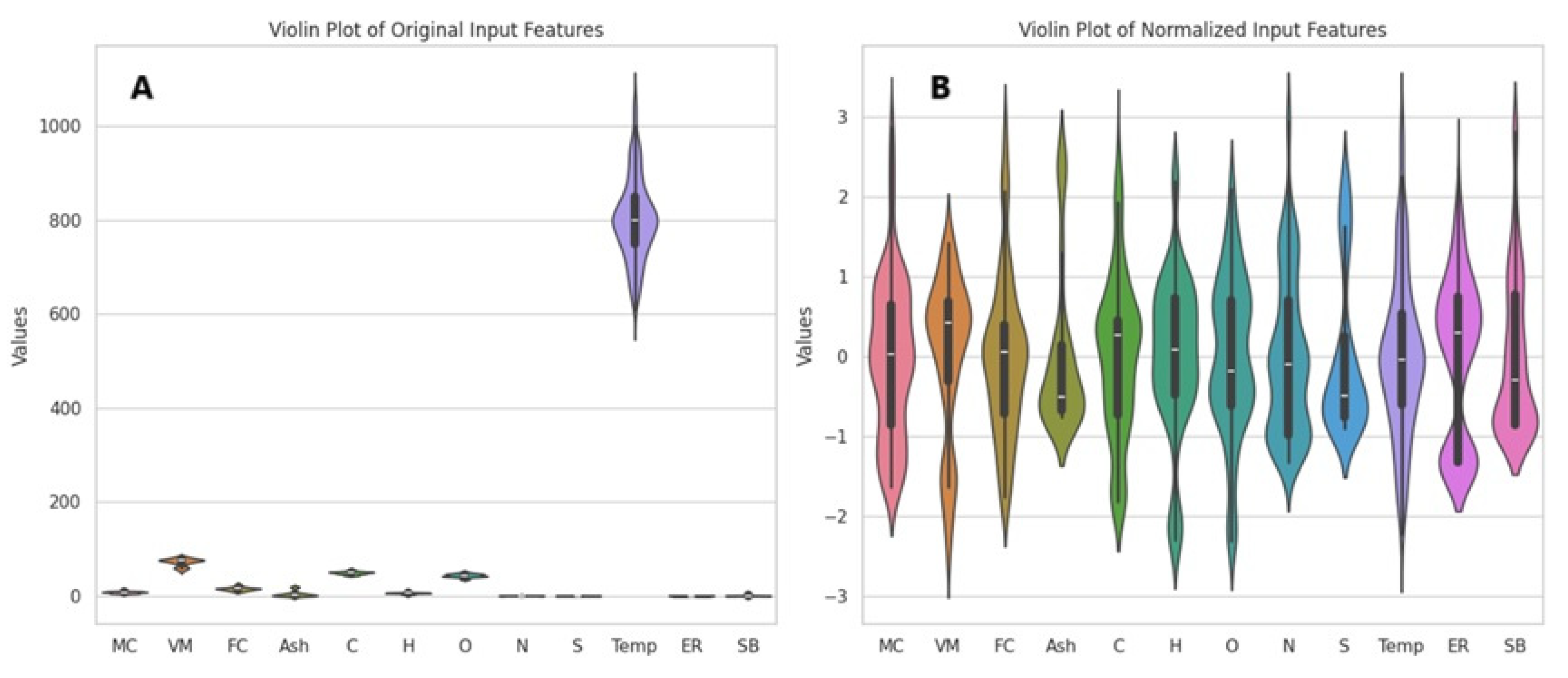

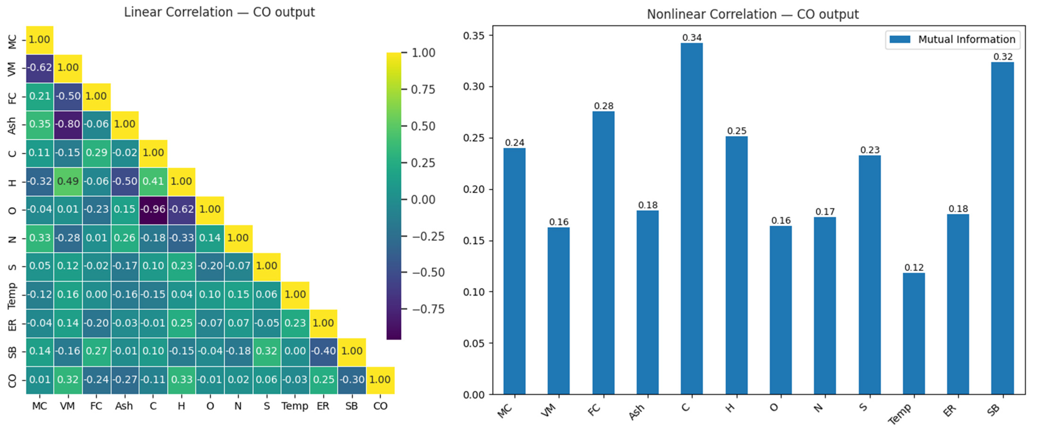

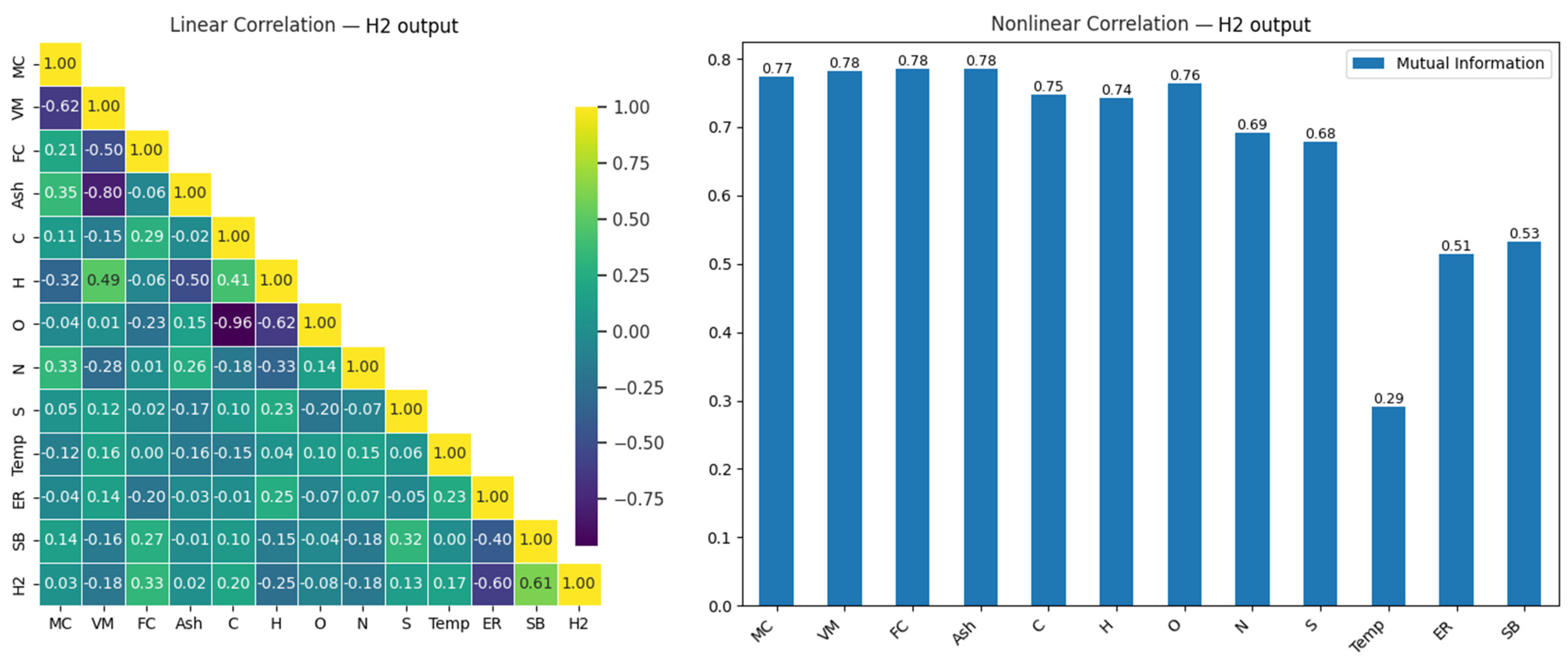
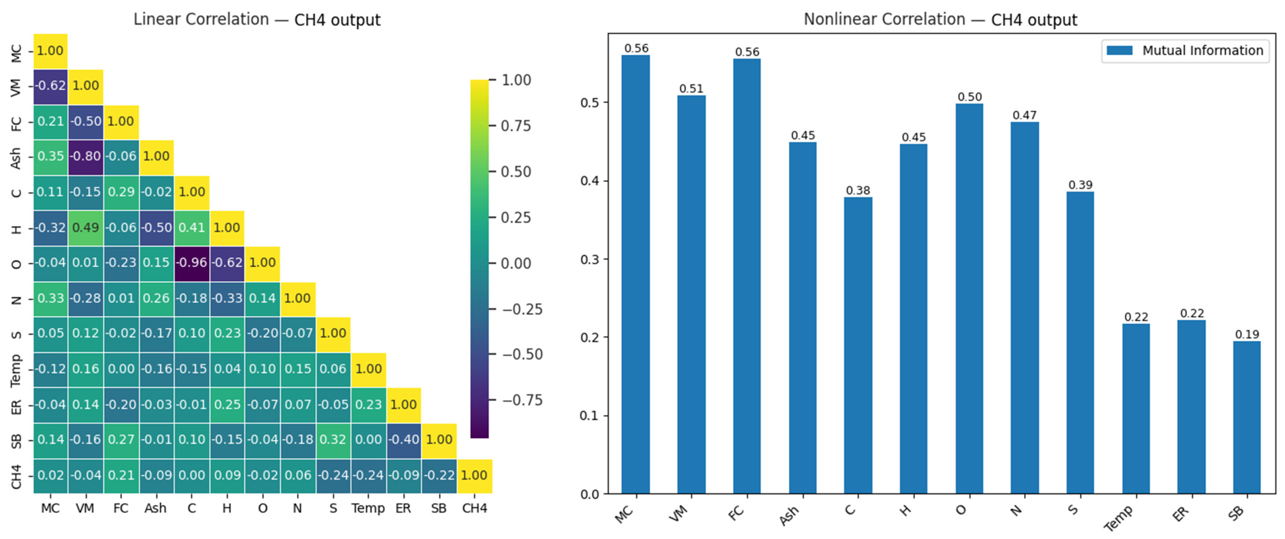

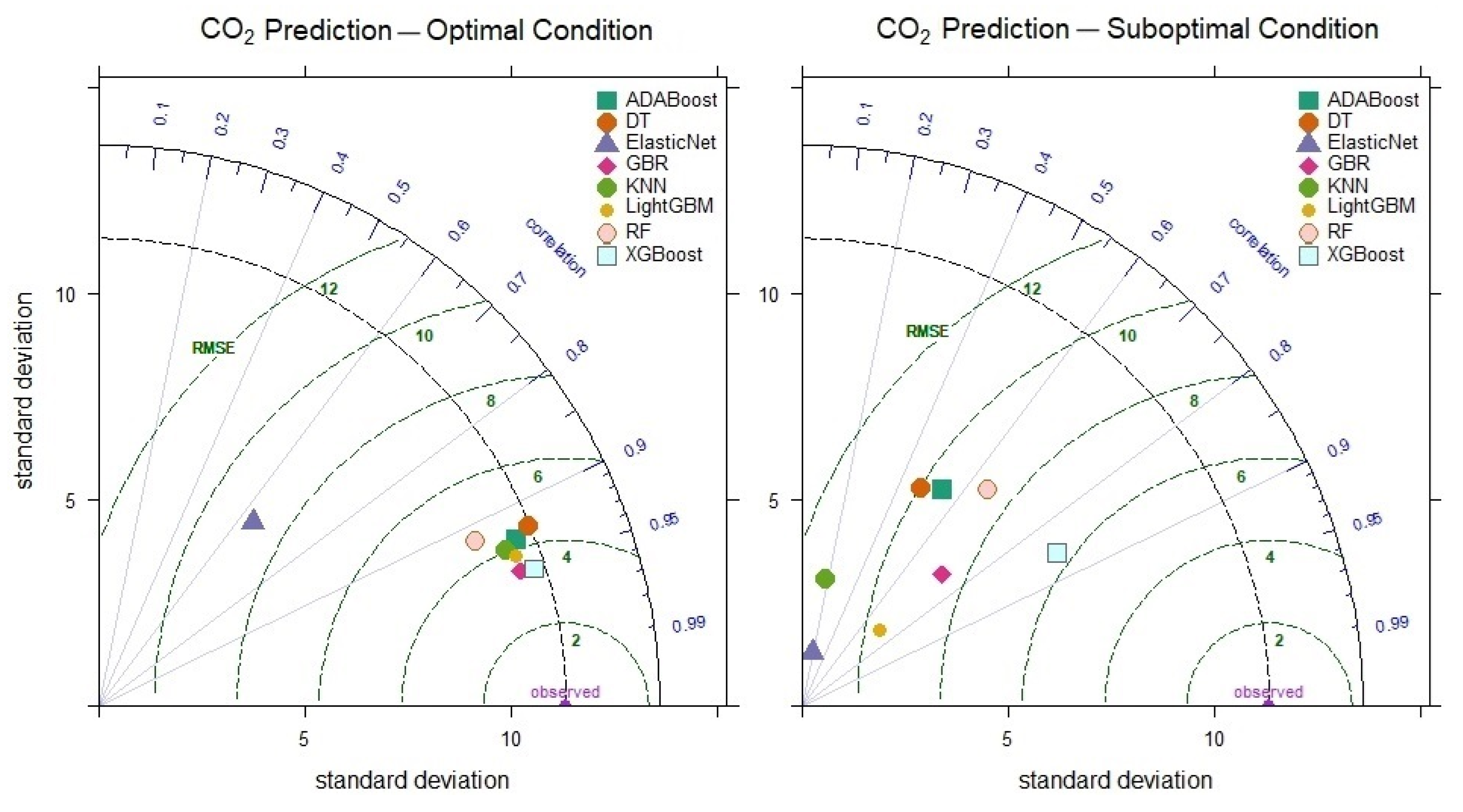
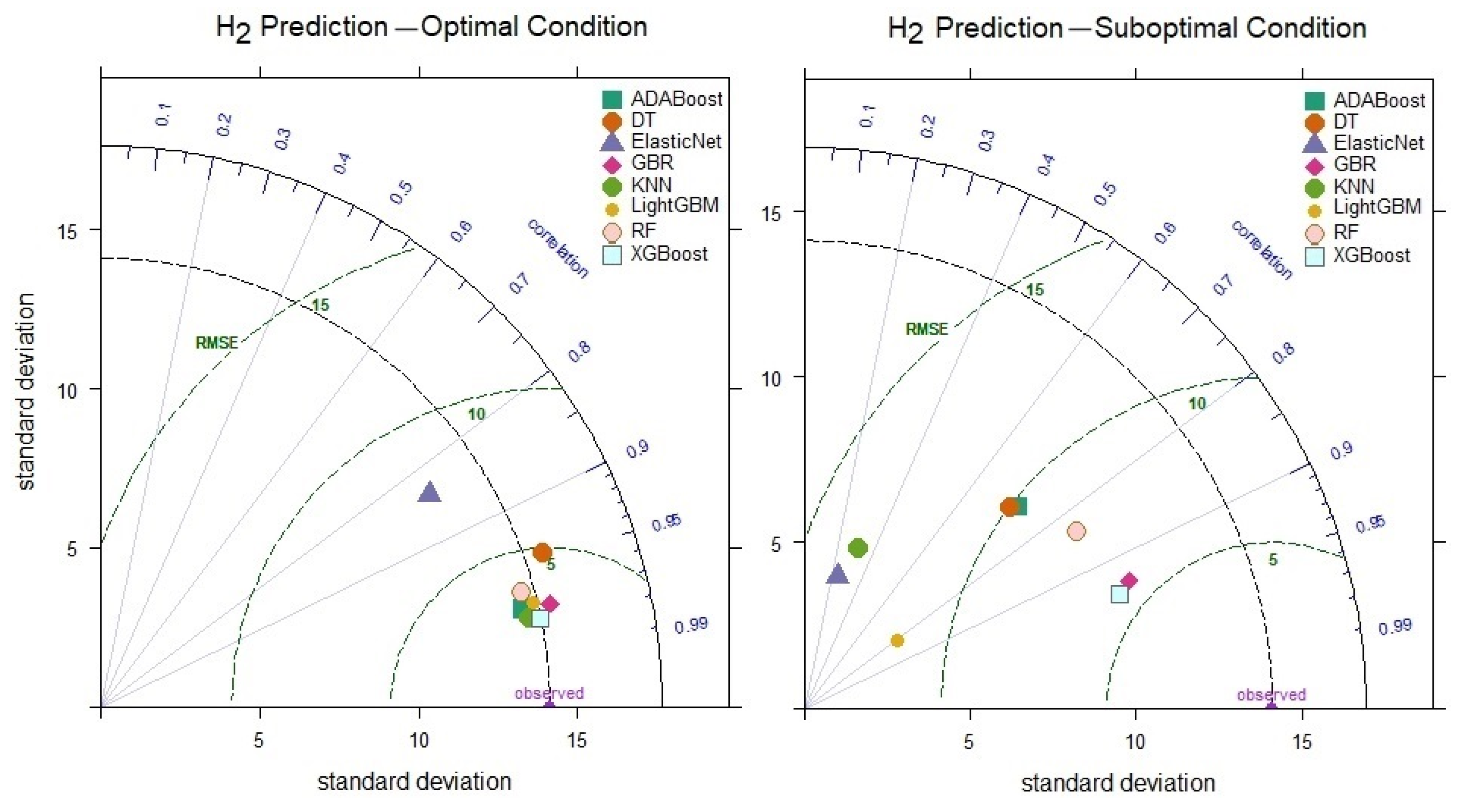
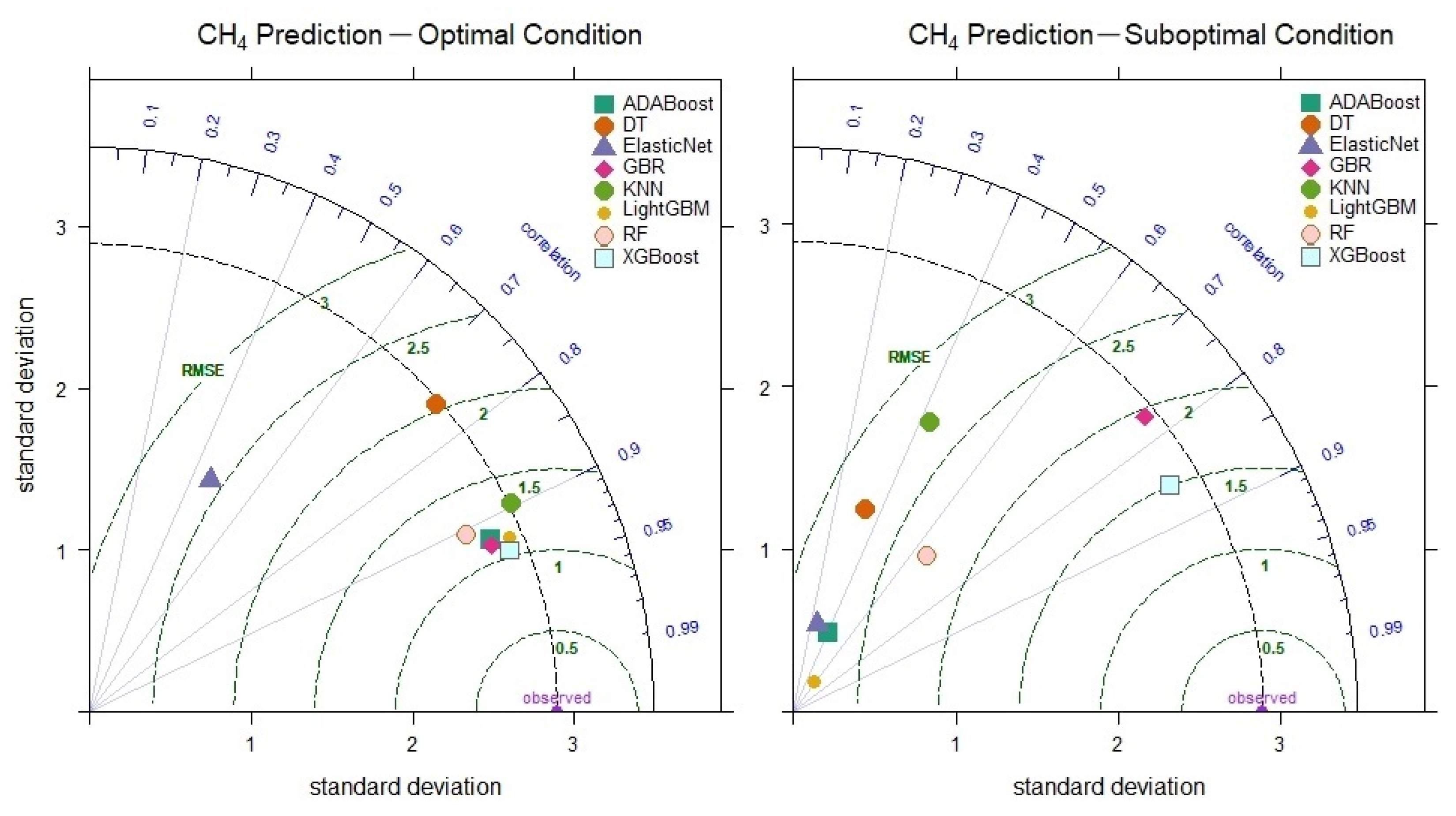
Disclaimer/Publisher’s Note: The statements, opinions and data contained in all publications are solely those of the individual author(s) and contributor(s) and not of MDPI and/or the editor(s). MDPI and/or the editor(s) disclaim responsibility for any injury to people or property resulting from any ideas, methods, instructions or products referred to in the content. |
© 2025 by the author. Licensee MDPI, Basel, Switzerland. This article is an open access article distributed under the terms and conditions of the Creative Commons Attribution (CC BY) license (https://creativecommons.org/licenses/by/4.0/).