Assessment of Fatigue Life and Failure Criteria in Ultrasonic Testing Through Thermal Analyses

Abstract

An experimental study was conducted to analyze temperature evolution during very high cycle fatigue tests. The temperature–number of cycles (T–N) curve is typically divided into three phases: Phase I—a rapid temperature increases at the start of the test, Phase II—temperature stabilization, and Phase III—a sharp temperature rise at the test’s end, coinciding with specimen fracture. The high frequencies used in ultrasonic fatigue testing can induce self-heating in specimens, but the thermal effects are not yet fully understood. Temperature is known to influence the fatigue performance of materials. To explore this, specimens were subjected to varying stress levels and intermittent loading conditions while monitoring temperature evolution using infrared thermography. The T–N curves were obtained, and S–N curves were constructed for specimens tested at room temperature. All tests were performed under fully reversed loading conditions. The experimental data were used to evaluate models commonly applied in conventional fatigue testing. Additionally, the temperature gradient at the beginning of the ultrasonic fatigue test and the heat dissipation per cycle were estimated and analyzed as potential fatigue damage parameters. These findings indicate that parameters derived from the T–N curve have significant potential for predicting very high cycle fatigue life.

1. Introduction

Fatigue is progressive damage to the material under cyclic stress. It is an irreversible process in which plastic deformations accumulate in the material as it undergoes repeated loading cycles. Fatigue is categorized into low cycle (LCF), high cycle (HCF), and very high cycle fatigue (VHCF) regimes depending on the number of cycles to failure. LCF is characterized by a short fatigue life (N_f < 10³–10⁴) and stress levels that are between the ultimate strength (σ_u) and yield strength (σ_y) of the material. In the HCF regime, the stress values are below the σ_y of the material. There is no presence of macroscopically plastic deformations, only elastic deformations [1,2].

An extension of the S–N curve was proposed by Bathias [3,4] in 1999, when he declared that “There is no infinite fatigue life in metallic materials”, emerging the VHCF region, which comprises a number of cycles between 10⁶–10⁷ and 10⁹–10¹⁰.

Similar to HCF, the VHCF regime also exhibits macroscopically elastic deformations. In certain cases, cracks may initiate internally, resulting in the formation of FGA (fatigue granular area) and fish-eye patterns.

This study was made possible through extensive experimental results obtained using an ultrasonic frequency fatigue machine (20 kHz), which significantly reduced testing time [3,4,5,6]. The development of this technology has greatly advanced the evaluation of very high cycle fatigue (VHCF), becoming crucial for designing structures and mechanical components capable of enduring high cycle counts throughout their service life.

As mentioned, VHCF testing employs ultra-high-frequency loading, reducing test duration. However, elevated stress levels during testing can lead to significant temperature increases in the specimens, a phenomenon documented by several authors [6,7,8,9,10,11]. Under certain conditions, excessive heating may result in specimen burning, adversely affecting the material’s fatigue performance.

The prediction of fatigue life for metallic materials remains a topic of ongoing research, with most studies relying on experimental data to fit predictive models. Traditionally, the fatigue life is estimated using the S–N curve, a method introduced by Wöhler that is widely applied and well established in the literature. However, the S–N curve can be influenced by various operational factors, including frequency, temperature, stress levels, and environmental conditions [1,2,12].

Fatigue occurs when mechanical energy (work input) is transferred to a specimen. Part of this energy accumulates within the material, while the rest dissipates as heat, causing temperature increases during fatigue testing. When the specimen’s temperature stabilizes, it indicates that the energy is fully dissipated [13,14,15].

Recently, thermodynamic approaches to understanding fatigue behavior have gained attention, particularly for analyzing self-heating phenomena in materials subjected to cyclic loading. These studies primarily focused on low cycle fatigue (LCF) and high cycle fatigue (HCF) regimes, proposing models correlating fatigue behavior with energy dissipation and temperature evolution.

This paper aims to investigate temperature evolution, fatigue performance, and material behavior under VHCF testing using thermodynamic concepts. The objectives include the following:

• Conducting experimental tests under various stress levels and intermittent loading conditions (different pulse and pause times) while monitoring temperatures using infrared (IR) thermography to develop temperature (T)–number of cycles (N) curves.
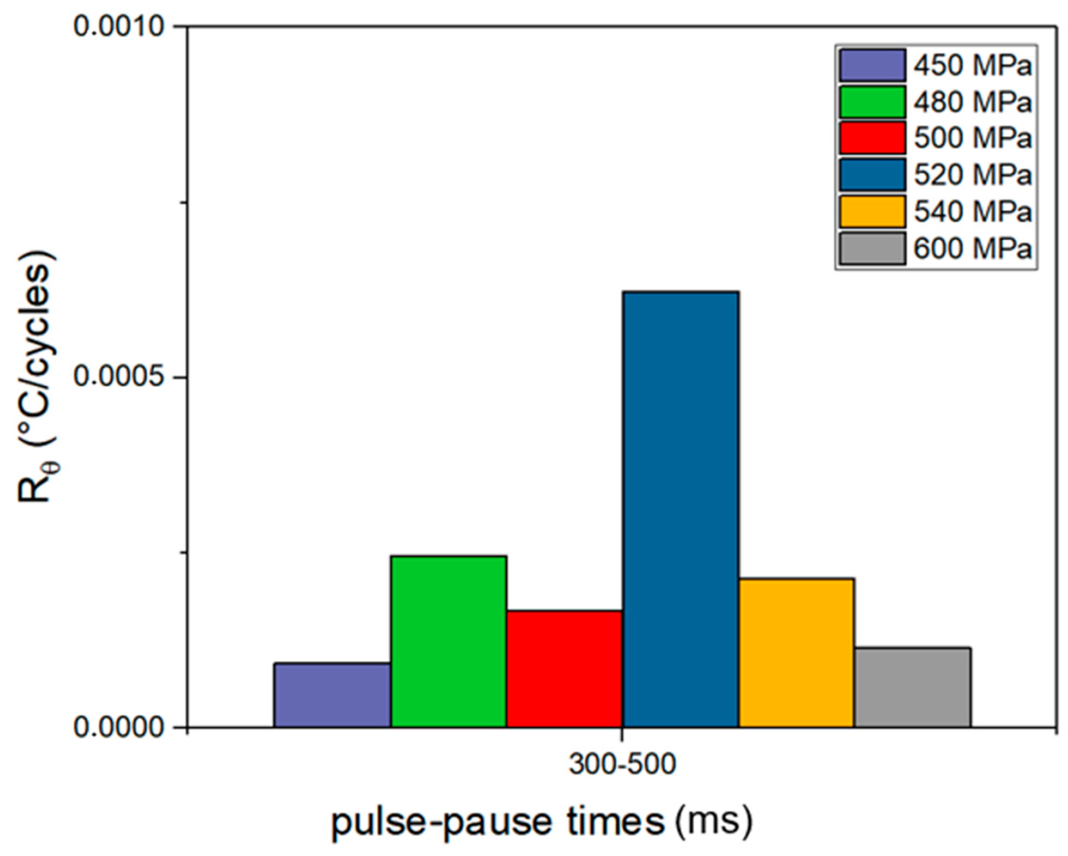
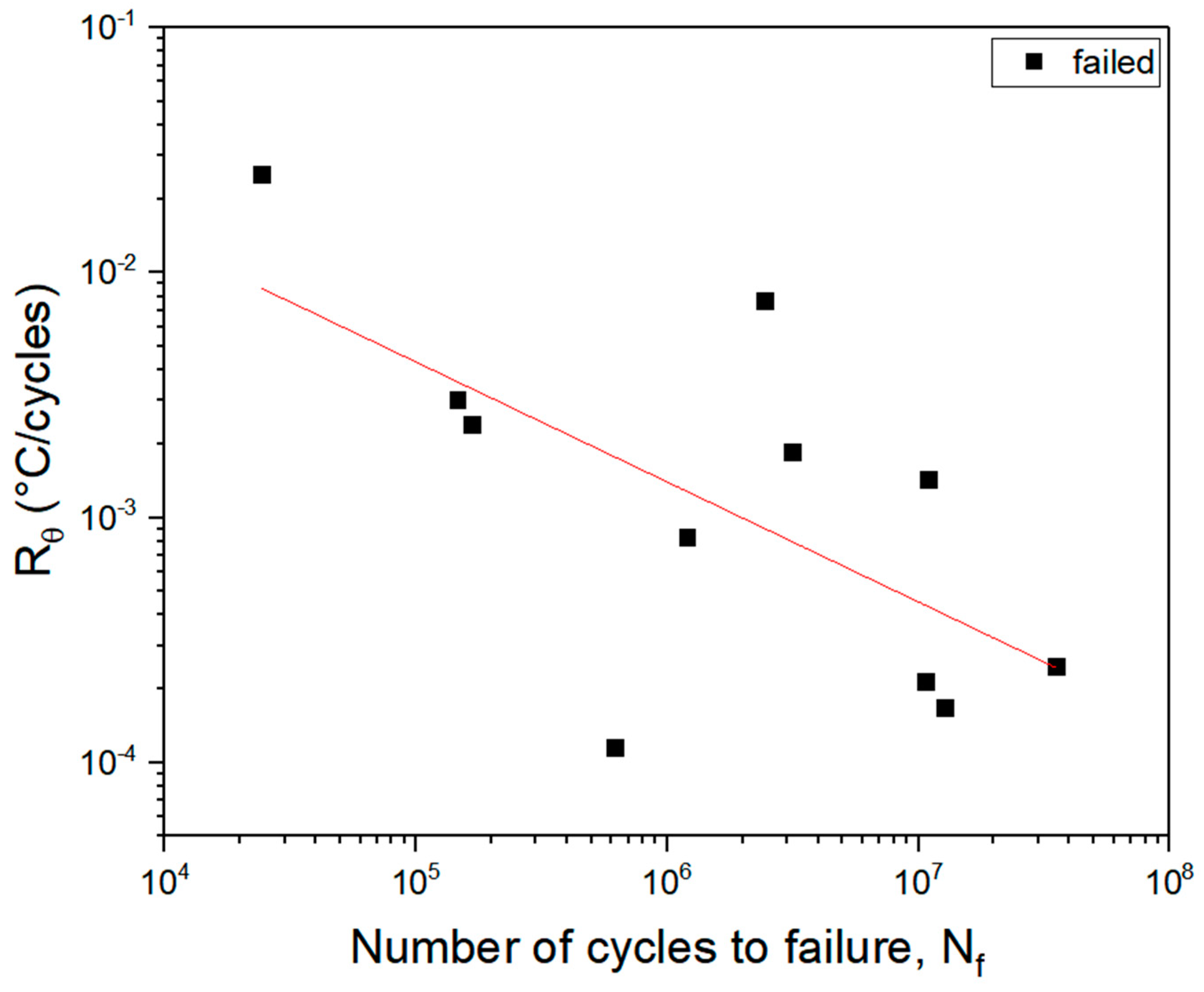
• Estimating temperature gradients at the onset of fatigue testing (R_Θ) from the T–N curves and analyzing their dependence on stress levels and effective frequency (f_eff).
• Deriving S–N curves independent of temperature effects.
• Applying fatigue failure criteria models to ultrasonic frequency test results to identify the model that best aligns with experimental data and determine the most suitable parameters for representing fatigue damage in VHCF testing.

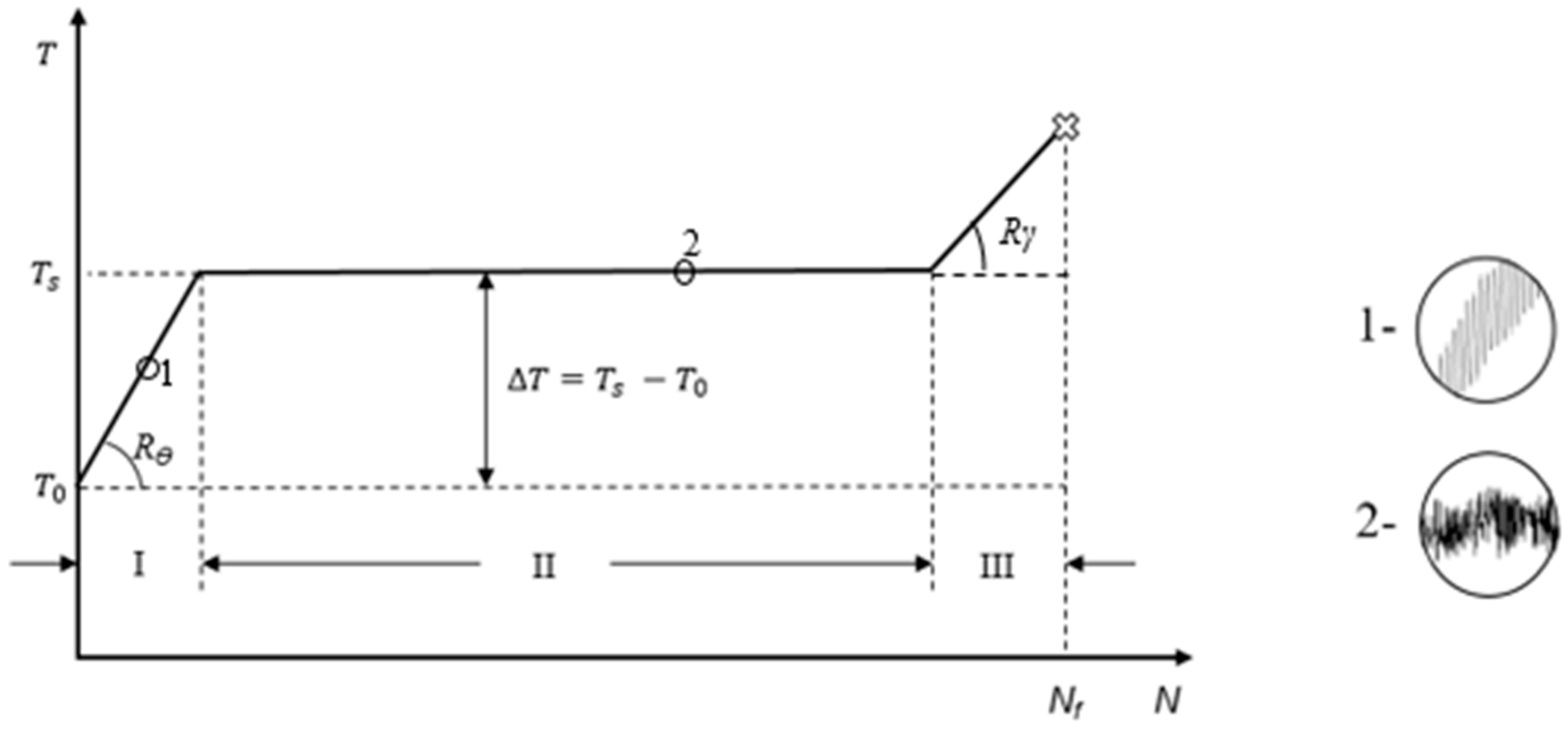
2. Fundamentals for Fatigue and Temperature Rise

Thermodynamic approaches related to mechanical fatigue have been extensively reported in the literature [12,13,14,15,16,17,18,19,20,21,22,23] to predict fatigue life. Some methods have been tested using temperature parameters derived from the T–N curve. Meneghetti [15,18,19] specifically correlated fatigue life with heat dissipation. However, these methods have primarily been applied to low cycle fatigue (LCF) and high cycle fatigue (HCF) regimes.

The temperature evolution during fatigue testing is represented by the T–N curve, as shown in Figure 1. This curve is divided into three distinct phases, each representing a specific stage of the fatigue process [12,13,14,15,16,17,18,19,20,21,22,23]:

• Phase I: At the start of the test, the specimen’s temperature rises rapidly from the initial room temperature (T₀) to the stabilized or steady-state temperature (T_s).
• Phase II: The temperature variation is minimal, indicating that the specimen has reached the steady-state temperature (T_s). According to the literature, this phase accounts for the majority of the specimen’s fatigue life.
• Phase III: The temperature rises sharply again but over a relatively small number of cycles. This phase marks the conclusion of the fatigue test, culminating in the specimen’s fracture.

Phase II tends to decrease and R_ϴ is more pronounced with the higher applied stress amplitude (σ_a) with constant operational frequency (Figure 2). This behavior is often described in low-frequency tests.

As it is known, fatigue is an irreversible process and the energy dissipation during the cyclic loading is responsible for the temperature increase at the beginning of the test. When the temperature achieves the T_s, the thermal energy is totally dissipated [12,16,17].

Table 1. Fatigue failure criteria models (adapted by [16]).

Failure Criteria	Equations		Reference	Behavior
Jiang et al.	$N_f^m=C \Delta T$ $m and c are material constants$		[22]	Is inapt for tests that do not exhibit phase II
Fargionne et al.	$\varnothing ={\int }_0^{N_f}\Delta T dN=constant$		[23]
Meneghetti et al.	1° Law of Thermodynamics:	$N_f=C Q_{cyc}^m$	[15,17,18,19]	Requires only phase I and it is applicable to any geometry and type of loading
	$Q_{cyc}={\displaystyle \frac{ \rho c_p{R}_{\theta }}{f}}$	$\rho =density \left({\displaystyle \frac{\mathrm{k}\mathrm{g}}{{\mathrm{m}}^3}}\right)$ $c_p=specific heat capacity \left({\displaystyle \frac{\mathrm{J}}{\mathrm{k}\mathrm{g}}}°\mathrm{C}\right)$ $f=frequency \left({\displaystyle \frac{\mathrm{c}\mathrm{y}\mathrm{c}\mathrm{l}\mathrm{e}\mathrm{s}}{\mathrm{s}}}\right)$
Amiri and Khonsari	$N_f=c_1{R}_{\theta }^{c_2}$ $c_1 and c_2 are material constants$		[20,21]

exhibits the main models based on the T–N curve to estimate the fatigue life. These models were obtained from LCF and HCF tests [16].

Jiang et al. [22] correlated fatigue life with the steady-state temperature T_s, measured from the initial room temperature T₀. This model can be applied if the test demonstrates a well-defined steady-state temperature and concludes with specimen fracture.

Fargionne et al. [23] proposed that the area beneath the T–N curve remains constant and is unaffected by the stress amplitude σ_a, provided that the steady-state temperature is achieved during the test.

Meneghetti [15,17,18,19] conducted extensive fatigue testing at low frequencies using plain and notched specimens under low- and high-cycle-fatigue regimes. Meneghetti found that the heat dissipation per cycle (Q_cyc) is a material property independent of specimen geometry, test frequency, and operational conditions, making it a potential fatigue damage parameter. Q_cyc is grounded in the first law of thermodynamics, with its analytical derivation detailed in [13,14]. Initially, Q_cyc was reported as being proportional to the temperature slope at the beginning of the cooling stage [15,17,19]. However, Jang and Khonsari [21] observed that the temperature slope at the start of the test (t = 0) matches the slope observed during the cooling stage. This approach enables the estimation of fatigue failure based on the heat generated and converted from mechanical energy during the fatigue process.

The most recent model, developed by Amiri and Khonsari [16,20], is notably straightforward. It relies solely on the temperature increase rate at the start of the test (R_Θ). Their findings indicate that fatigue life can be predicted using a universal curve, irrespective of stress conditions. They validated this model for two steel types under torsion, rotating bending, and bending tests, highlighting the temperature rise slope as a reliable predictor of fatigue life.

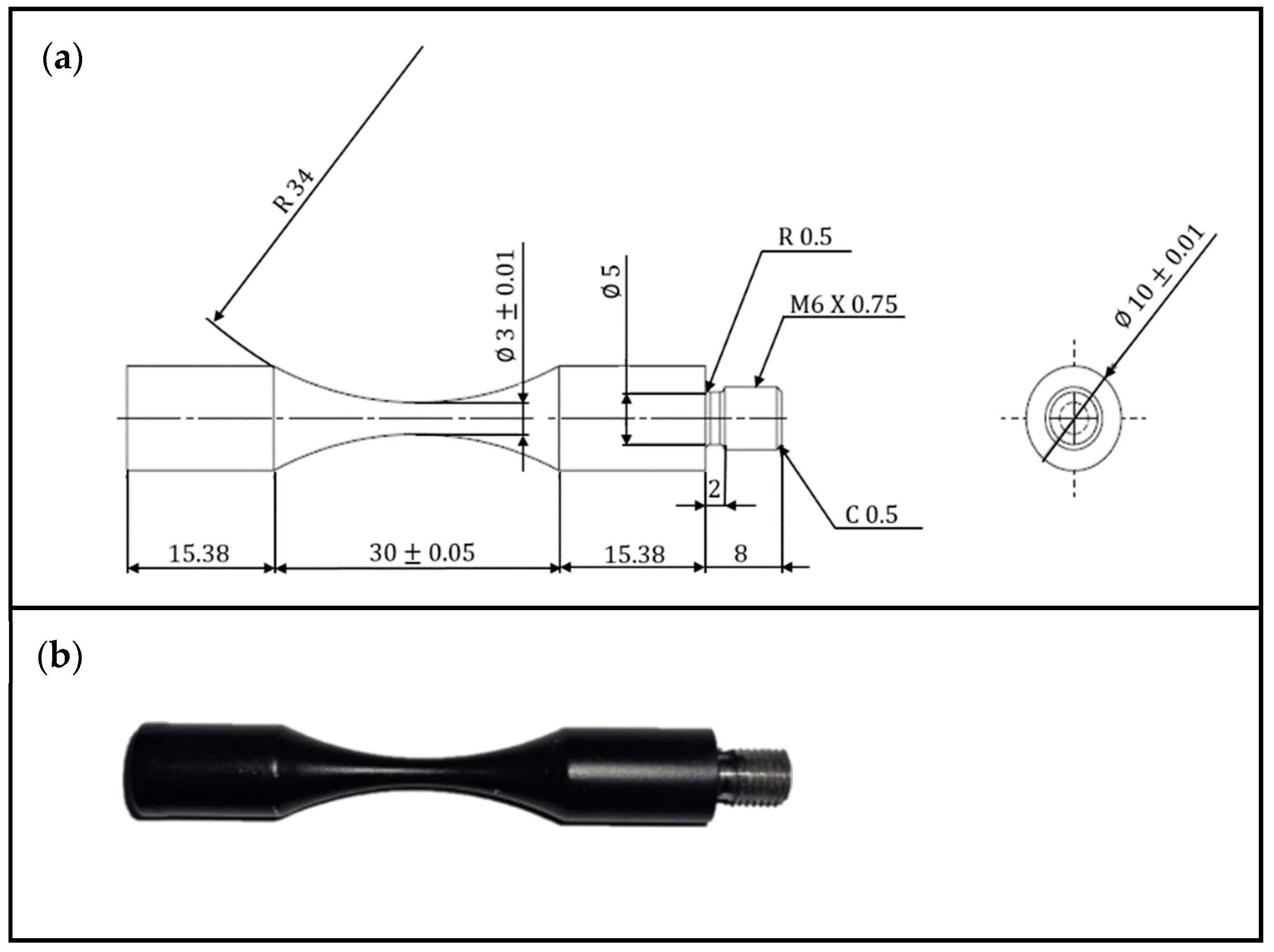
3. Materials and Methods

3.1. Materials

The steel used in this study was 34CrNiMo6, which is used for several mechanical components. The machined specimens were obtained directly from the failed crankshaft under study. The chemical composition and mechanical properties were determined using Optical Emission Spectroscopy and tensile testing, respectively, and are presented in

Table 2. Chemical composition with main elements.

Steel	Fe (%)	C (%)	Cr (%)	Mo (%)	Ni (%)
34CrNiMo6	95.1	0.38	1.51	0.24	1.75

and

Table 3. Mechanical properties.

Steel	σu (MPa)	σy (MPa)	E (GPa)
34CrNiMo6	900	760	207

. The steel has a density of 7870 kg/m³ and a specific heat capacity of 475 J/kg °C.

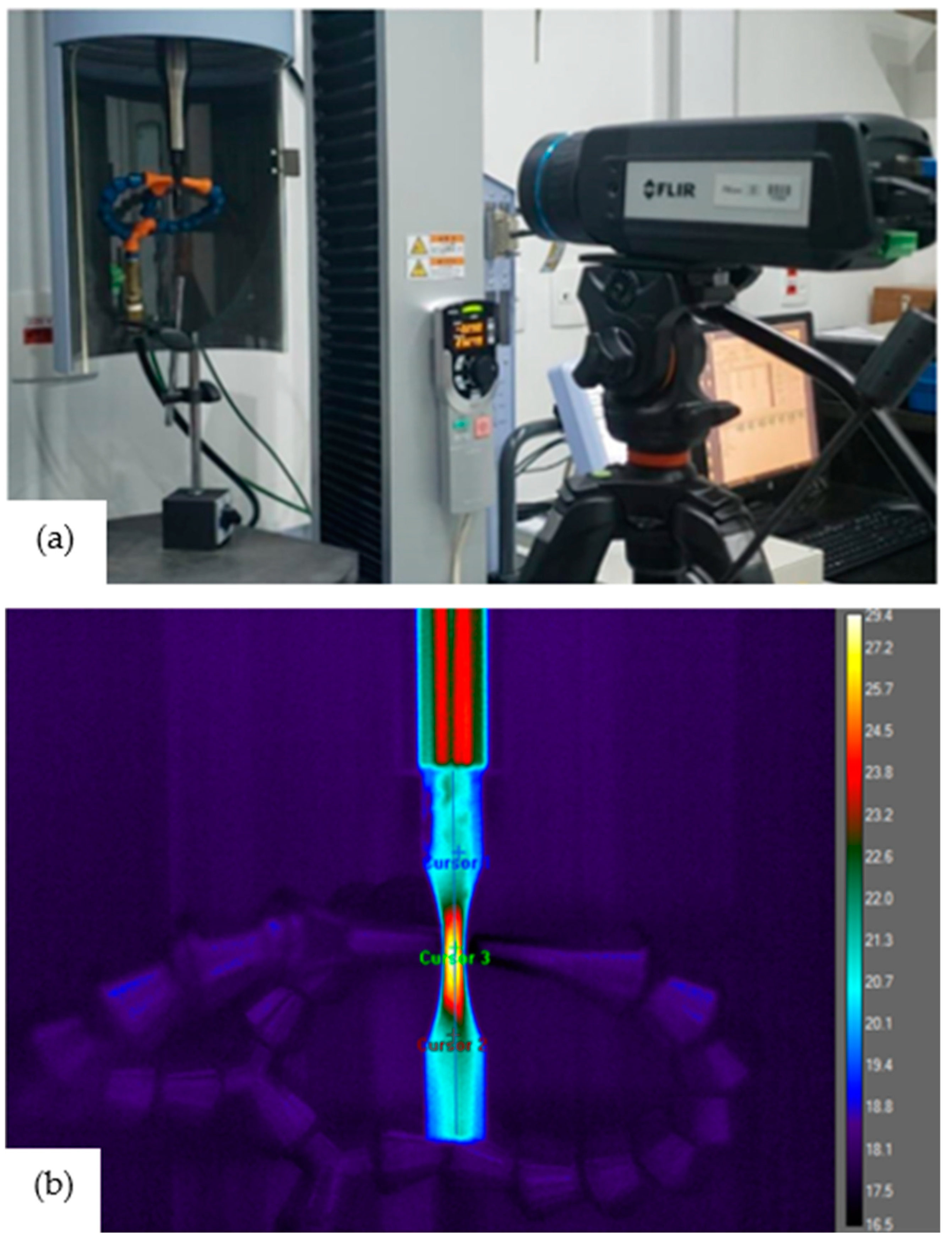
3.2. Methods

To conduct the tests, a black coating spray paint was applied to the specimens to increase their emissivity. This step was essential for improving the accuracy of temperature measurements. Figure 3a shows the specimen geometry, while Figure 3b displays the specimen after applying the black coating.

The experiments were conducted using a VHCF testing machine, model Shimadzu USF-2000A (Kyoto, Japan). Temperature monitoring was performed with an infrared (IR) camera, model A655SC (FLIR, Wilsonville, OR, USA), focusing on three points along the reduced section of the specimen. Additionally, a straight-line measurement was included to track temperature variations across the specimen. This camera features a temperature measurement range of −40 °C to +150 °C and an accuracy of ±2 °C or ±2% of the reading (

Table 4. Parameters of the thermography experiments [6].

Distance of camera to specimen	0.5 m
Room temperature	20 °C
Emissivity	0.93
Frames per second	100
Temperature range settings	−40 to 150 °C; 100 to 650 °C; 300 to 2000 °C

). It provides an average sample over several cycles, which is enough to observe temperature trends.

Ultrasonic fatigue tests were supported by a cooling system and primarily conducted with intermittent loading to enhance temperature control. The high testing frequency, which enables rapid testing, can lead to self-heating of the specimen, potentially accelerating the damage process. The cooling system is a type of air compressor that has a tank capacity of around 50 L, a pressure that can go up to 10 bar (145 psi), and an airflow of around 250 to 350 L per minute (L/min).

Figure 4a illustrates the ultrasonic fatigue testing setup along with the IR camera, while the corresponding thermogram is shown in Figure 4b. The parameters used for the thermography experiments are summarized in Table 4.

Specimens were tested under fully reversed loading conditions (R = −1) at various stress levels using a pulse–pause technique. Stress levels were chosen as a percentage of the material’s ultimate strength (σ_u), ranging from 30% to 66%, with varying pulse and pause durations.

Additionally, tests were conducted both with and without cooling using a pulse–pause of 110–500 ms, targeting a total of 10⁶ cycles. For these specific tests, a lower effective frequency was used to minimize wear on the testing machine and specimens. These experiments aimed to evaluate the influence of compressed air cooling on temperature evolution during the VHCF tests.

Table 5. Experimental conditions with IR camera.

Pulse–Pause (ms)	feff (Hz)	σa (MPa)
300–200	11,600.93	270
		315
		360
		405
200–200	9680.54	270
		315
		360
		405
200–300	7598.78	270
		315
		360
		405
300–500	7521.63	450
		480
		500
		520
		540
		600
110–500	3278.68	270
		360
110–500	3278.68	270
(no cooling)		360

outlines the experimental conditions, including pulse–pause settings, corresponding effective frequencies (f_eff), and stress amplitudes (σ_a). Tests with pulse–pause settings of 300–200 ms, 200–200 ms, 200–300 ms, and 300–500 ms were conducted to approximately 10⁷ cycles.

The S–N curve was performed using pulse–pause times with 300–500 ms that provided experiment results without temperature effect. The tests were conducted at room temperature (RT), R = −1, and with air cooling.

Table 6. Experimental conditions to obtain the S–N curve.

Pulse–Pause (ms)	feff (Hz)	σa (MPa)
300–500	7521.63	360
		420
		440
		450
		460
		470
		480
		500
		520
		540
		600

shows the experimental conditions used to obtain the S–N curve.

4. Results

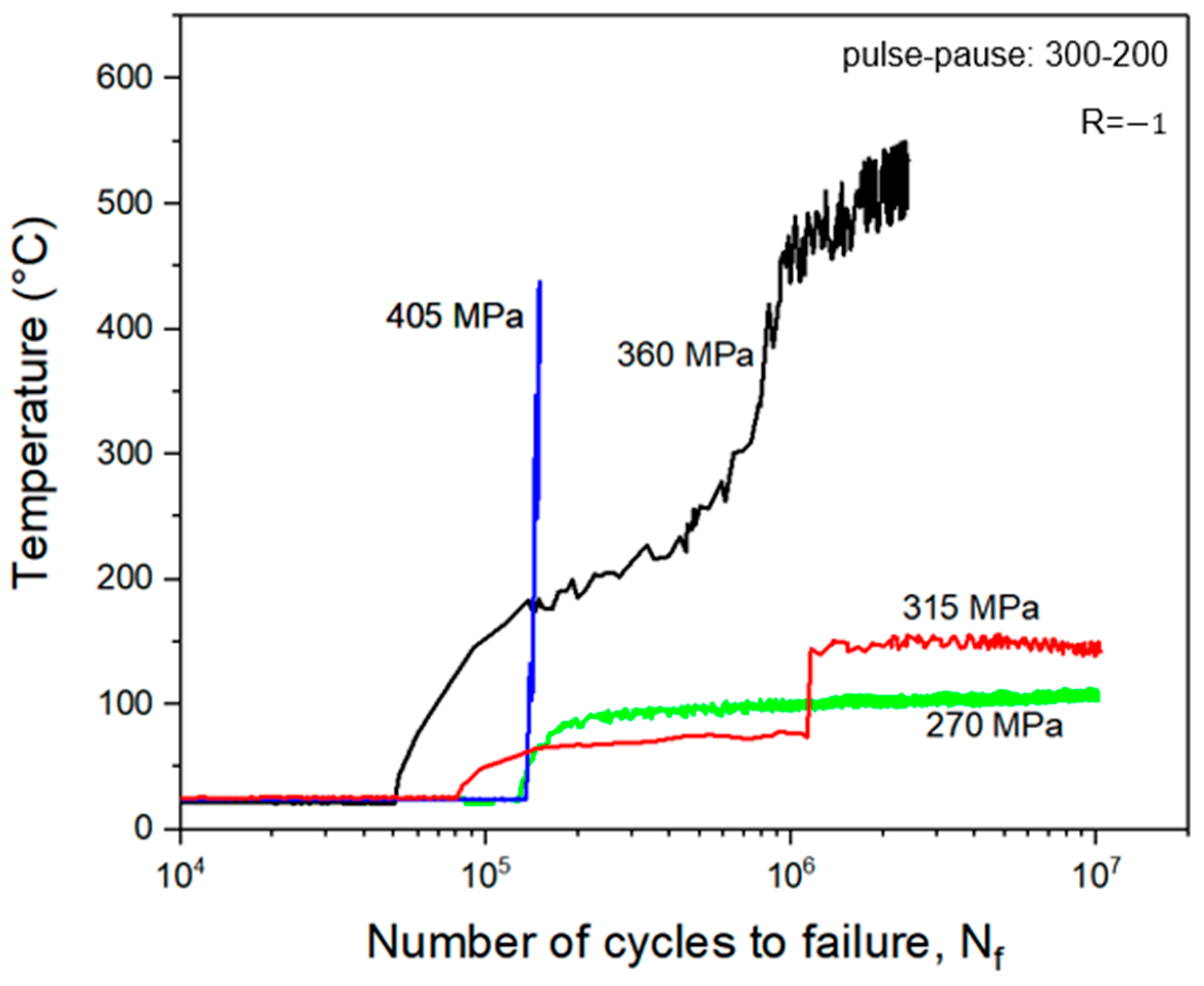
4.1. T–N Curves

The graphs and thermographic images obtained using the thermography method are shown in Figure 5, Figure 6, Figure 7, Figure 8 and Figure 9. These images illustrate the thermal gradients measured at the center of the specimen, where the maximum stress is concentrated. Figure 5, Figure 6, Figure 7 and Figure 8 display the T–N curves corresponding to identical stress levels under varying intermittent loading conditions.

These graphs highlight the significance of the pulse–pause technique in facilitating cooling during the tests. The influence of intermittent loading on each σ_a is evident. Longer pulse–pause durations result in higher temperatures at the center of the specimens.

Tests with a pulse–pause interval of 300–200 ms produced the highest temperatures across all stress levels, as anticipated. Specimens subjected to 45% and 40% of σ_u, equivalent to 405 MPa and 360 MPa, respectively, failed under these conditions, with temperatures exceeding 300 °C.

Figure 8 depicts the thermal gradients for a pulse–pause interval of 300–500 ms. This intermittent loading scheme was selected based on the initial results shown in Figure 5, Figure 6 and Figure 7. The test began at a stress level of 450 MPa, corresponding to 50% of σ_u. The thermal gradients indicated that the specimen maintained temperatures below 25 °C. Consequently, subsequent tests were conducted at higher stress levels, revealing that under this condition, even at 66% of σ_u, the specimens did not exhibit elevated temperatures. All tests maintained temperatures below 40 °C.

The thermal gradients shown in Figure 9 illustrate the effect of the cooling system during VHCF tests. Specimens without cooling did not reach a steady-state temperature until after 10⁶ cycles. In contrast, cooled specimens achieved steady-state temperature before completing 100,000 cycles. Cooling reduced the maximum temperature by approximately 45 °C at a stress amplitude of 360 MPa. At a stress level corresponding to 30% of the ultimate tensile strength (σ_u), air cooling reduced the temperature by 15 °C.

In comparison with previous results with higher f_eff, the specimens experienced significant temperature effects that compromised the material’s fatigue performance. In contrast, the 300–500 ms pulse–pause interval minimized temperature-related impacts, preserving the material’s fatigue capability.

Figure 10 highlights the influence of intermittent loading and stress levels on temperature rise. It is evident that higher stress amplitudes (σ_a) and increased loading frequencies result in a more pronounced initial temperature gradient (R_ϴ). For instance, the combination of 300–200 ms pulse–pause intervals and 45% σ_u produced the steepest temperature gradient at the start of the VHCF test.

However, Figure 11 shows that R_ϴ did not exhibit significant variation across conditions. Most R_ϴ values obtained for pulse–pause intervals of 300–500 ms were less than 5 × 10 ⁻⁴, whereas R_ϴ values from Figure 10 demonstrated magnitudes closer to 10⁻³.

4.2. S–N Curve

The S–N curve was attained considering tests in RT in order to avoid the temperature effect and its impact on fatigue performance. The results present higher scatter, which is expected for fatigue tests and mainly in VHCF, as illustrated in Figure 12. In fatigue tests, the materials can be affected by several conditions, but in ultrasonic fatigue tests, the influence of internal defects is more pronounced, and this is reflected in the dispersed results. It can be observed that higher stress levels achieve run-out in 10⁹ cycles. The σ_a equivalent of 40% of σ_u reached 2 × 10⁹ cycles and did not fail. Some stress levels presented fatigue life three orders higher in magnitude.

The material constants obtained by the Basquin equation are 816 for A and −0.0310 for B, and their relation is presented in Equation (1).

$$N_f=816{\left({\sigma }_a\right)}^{-0.0310}$$

(1)

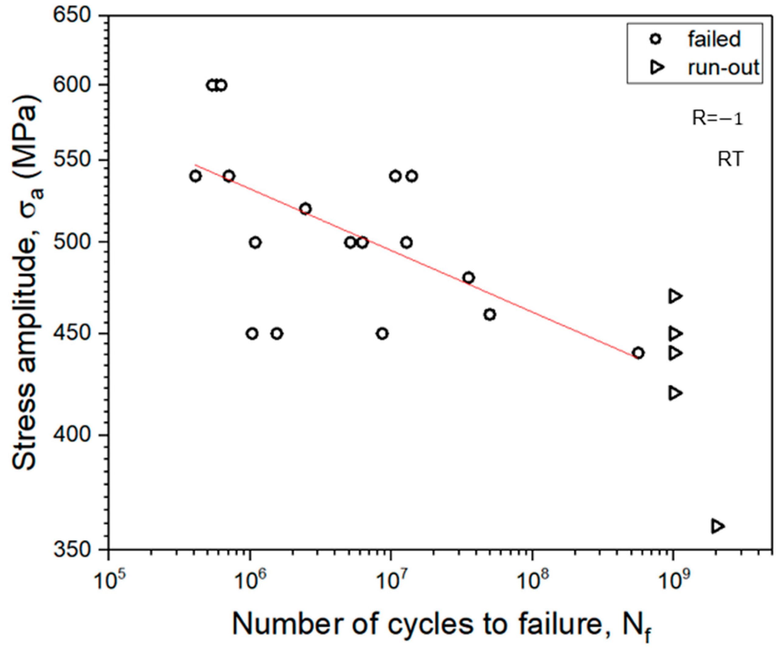
To evaluate the theoretical results, a correlation with predicted life (N_{f_pre}) and experimental life (N_{f_exp}) was applied and presented in Figure 13. Although there is higher scatter, most of the results are reliable (within 1:2 scatter bands) and also conservative.

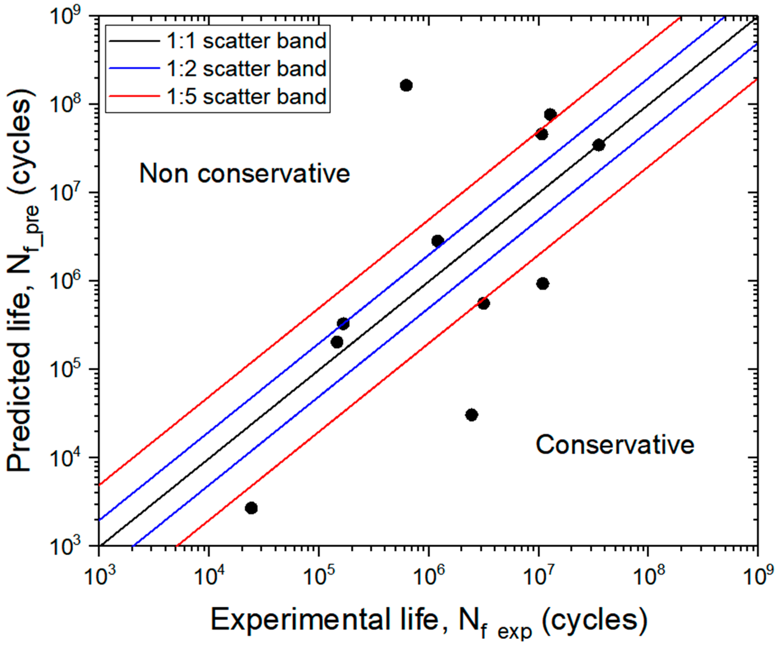
4.3. Model Evaluation

The main goal of this topic is to assess the models, described in Table 1, and identify which failure criteria provided a better agreement with ultrasonic fatigue results.

Jiang and Fargione’s models are inapt to apply in some cases. Most of the T–N curves did not present phase II, and using these models requires steady-state temperature. In light of this, these models are inappropriate to apply for the obtained T–N curves in this study.

With the results of the tested specimens failing, the heat dissipation (Q_cyc) was calculated based on the equation provided in Table 1 and associated with the number of cycles to failure (N_f) to obtain a more general failure criterion. As mentioned before, energy heat dissipation according to Meneghetti [15,17] is independent of the test frequency and the geometry of the specimen.

Figure 14 demonstrates the estimated Q_cyc related to the N_f. The results reveal that N_f decreases linearly with increasing Q_cyc. The fatigue function $Q_{cyc}=C{\left(N_f\right)}^m$ was obtained, where C and m are the constants of the material. The material in this study encountered values of C and m equal to 4.52 and −0.489, respectively.

With the purpose of verifying the accuracy of the predicted life results, they were evaluated and compared with the experimental results. Figure 15 presents this comparison and analysis for 1:5 and 1:2 scatter bands. According to Figure 14, the fatigue life estimated by the energy dissipation presented good accuracy. Around 90% of the fatigue data are within the scatter band and in the conservative region.

Although the specific heat capacity of steel varies with temperature, a constant value was used in this study to simplify the analysis. Future studies could benefit from incorporating temperature-dependent thermodynamic parameters to provide a more detailed understanding of their influence on VHCF performance [5,24,25,26,27].

The latest model by Amiri and Khonsari [16,20] was assessed by relating the R_ϴ with the N_f. R_ϴ data were estimated by the T–N curves and evaluated in Section 4.1. Figure 16 shows the R_ϴ vs. N_f. The constant parameters, c1 and c2, were attained by the fitted curve and have values of 1.21 and 0.489, respectively. It can be seen that the slope of the curve obtained by the fitted curve in Figure 14 and Figure 16 is the same. This is expected, given that Q_cyc is dependent on R_ϴ.

Similarly, in Figure 14, the predicted life estimated by R_ϴ presented in Figure 17 demonstrates great reliability. Most of the data are in the 1:2 and 1:5 boundaries.

4.4. Fracture Surfaces

In this section, selected specimens are used to demonstrate and compare the effect of temperature. As observed in the S–N curve, materials subjected to high stress levels were not significantly affected by temperature. However, specimens tested under pulse–pause conditions of 300–200 ms, 200–200 ms, and 200–300 ms, which failed before 10⁷ cycles, experienced significant temperature effects that reduced their fatigue life. This effect is evident on the fracture surfaces, which display different burn colors. Figure 18 shows the fracture surfaces obtained through stereoscopy, revealing the burned areas.

The fracture surface in Figure 18a failed at 1.20 × 10⁶ cycles, with 200–200 ms of pulse–pause and 360 MPa for σ_a. The specimen in Figure 18b was performed with 200–300 ms of pulse–pause under 405 MPa and failed at 1.66 × 10⁵ cycles. These specimens achieved temperatures above 350°C. It is important to highlight that 360 MPa under 300–500 ms of pulse–pause reached 2 × 10⁹ cycles without failure.

5. Conclusions

This study aimed to investigate the impact of intermittent loading on material fatigue performance and evaluate existing models based on temperature during very high cycle fatigue (VHCF) tests. The key findings are summarized below:

Temperature Effects:

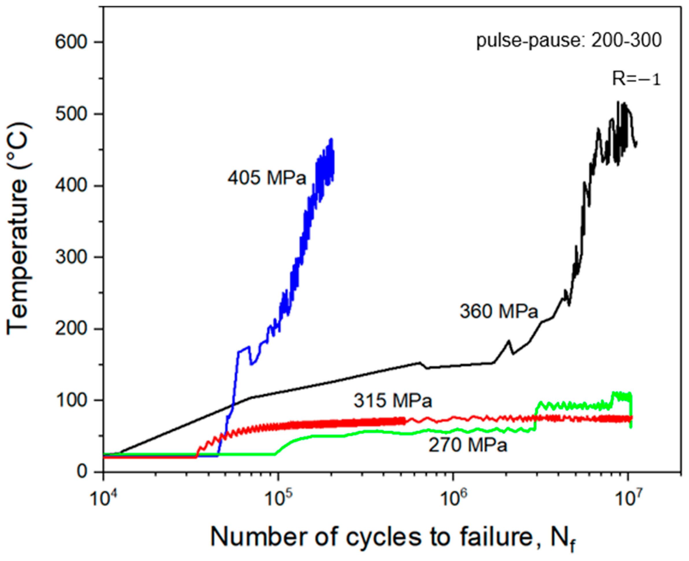
• In all T–N curves, temperature increases were observed as test time decreased.
• Specimens tested with intermittent loads of 300–200, 200–200, and 200–300 ms at stress levels of 40% and 45% σ_u showed that the maximum temperature exceeded 300 °C.
• Fatigue life was shortened in these cases compared with tests with a 300–500 ms pulse–pause time due to high temperatures.
• The steady-state temperature was not clearly defined for specimens that failed before reaching 10⁷ cycles.
• Specimens experienced an increase in surface temperature in relation to f_eff for a constant σ_a.
• Higher values of f_eff and σ_a led to a steeper temperature slope at the start of the test.
• S–N Curve and Fatigue Life:
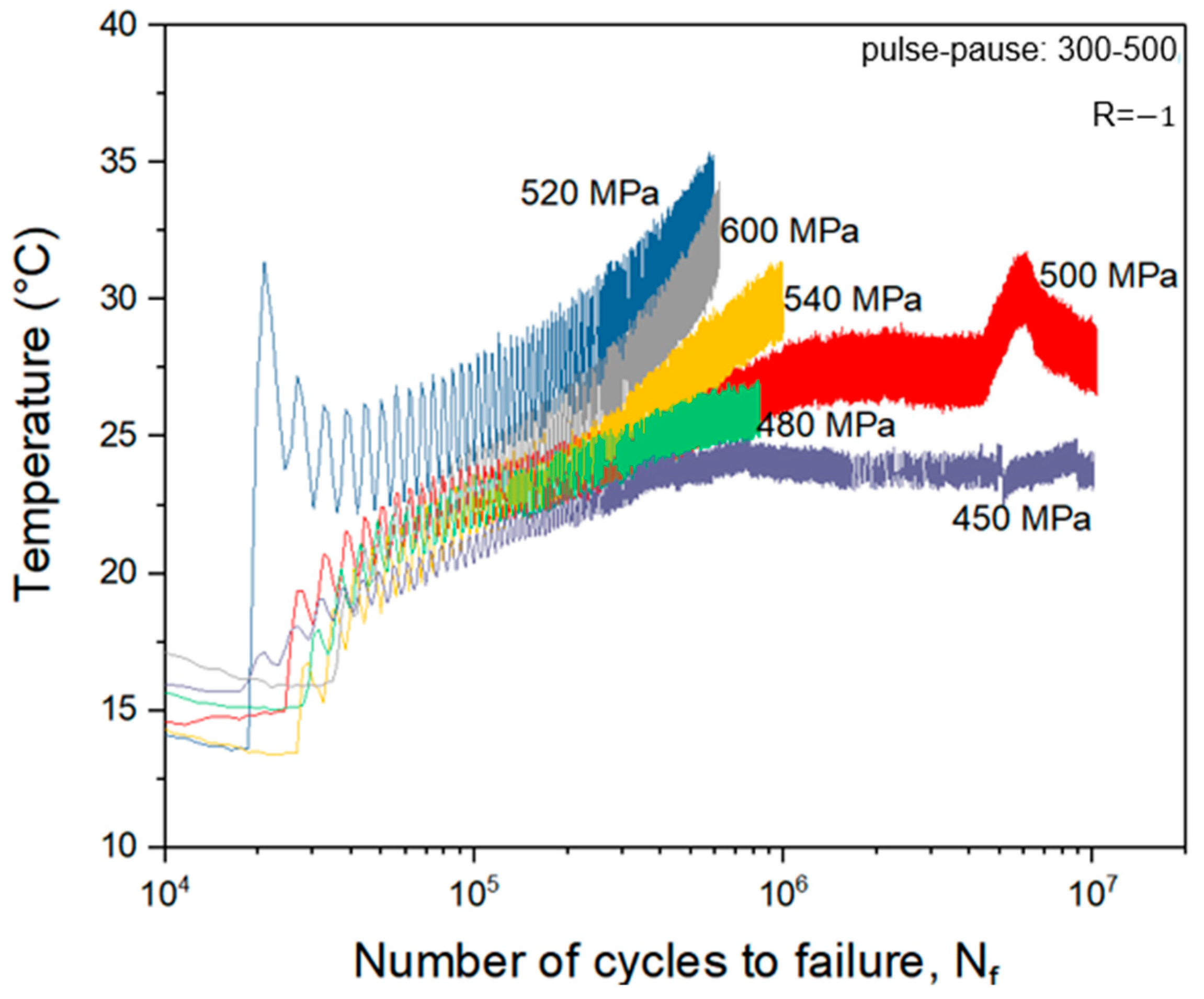
• An S–N curve was obtained under 300–500 ms pulse–pause conditions, exhibiting a higher level of scatter, as expected.
• The maximum temperature observed during these loadings was below 40 °C.
• The Jiang and Fargione models were found to be unsuitable for the experimental conditions of this study.
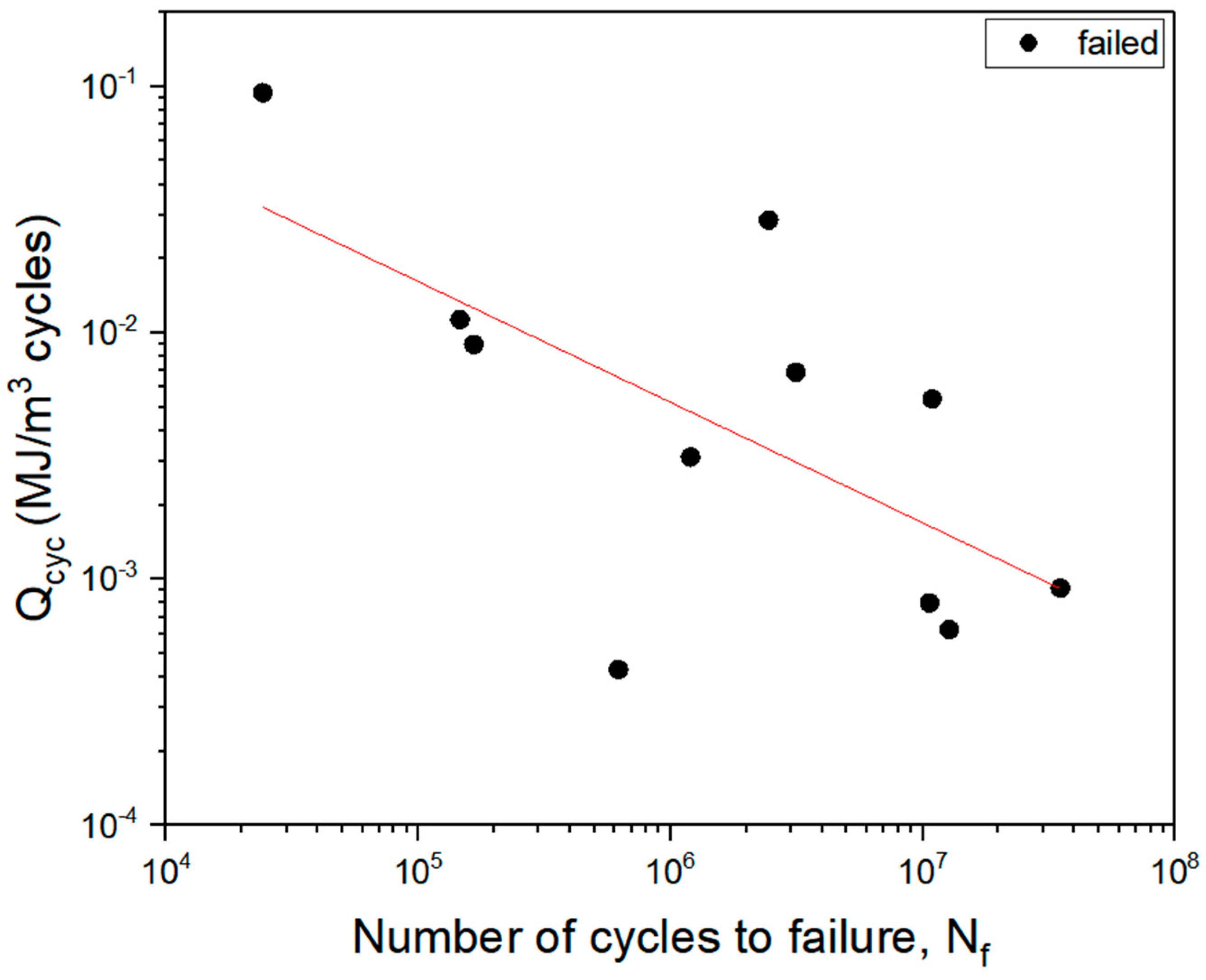
• The Q_cyc-N_f and R_ϴ-N_f curves aligned with those found in the literature for low-frequency tests, indicating that N_f increases as Q_cyc and R_ϴ decrease.

Model Accuracy and Prediction:

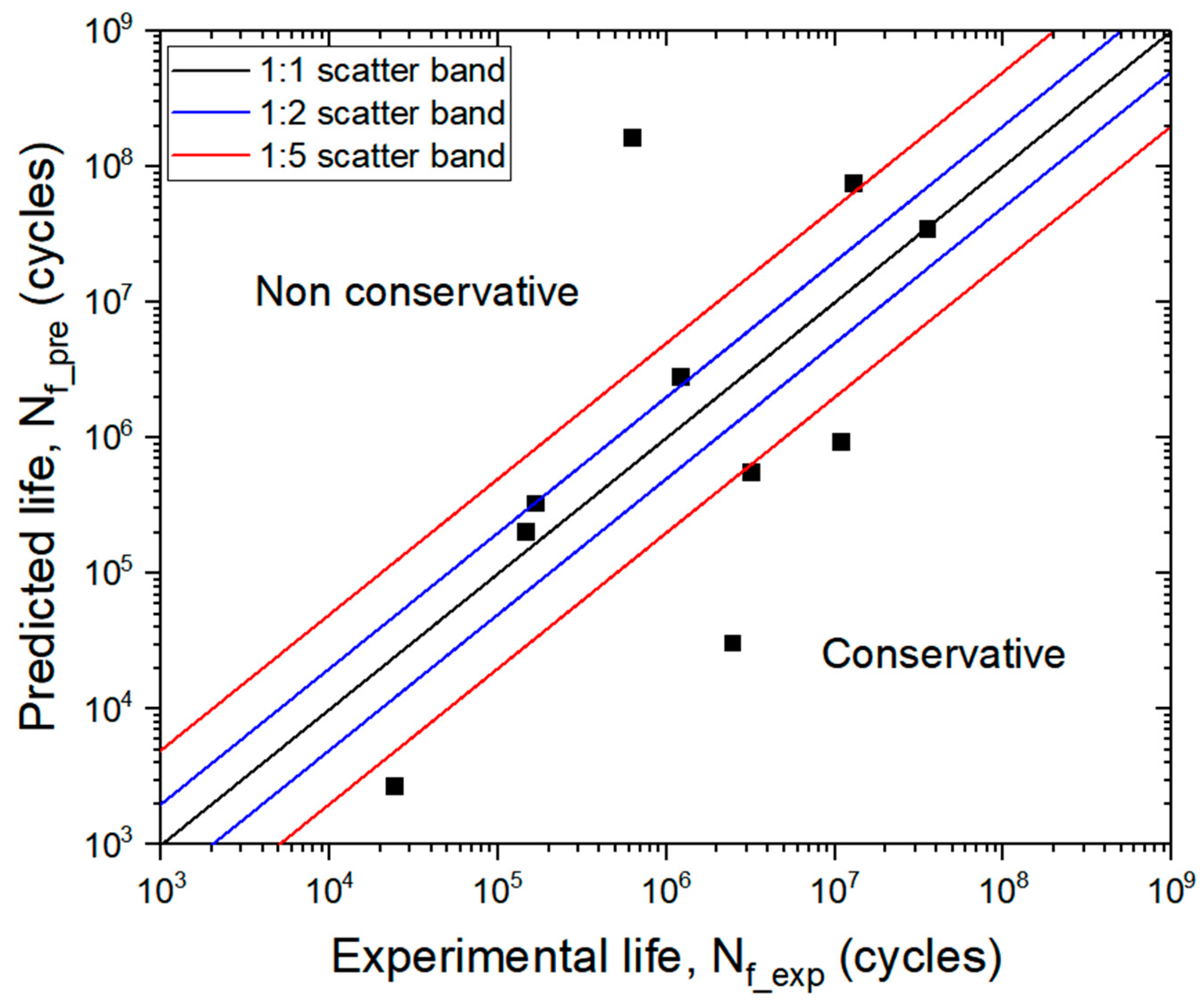
• Fatigue functions for both models were derived, with predicted results showing good accuracy compared with experimental tests.
• High scatter in ultrasonic fatigue tests may influence results.
• The Meneghetti and Amiri-Khonsari models showed strong potential for predicting fatigue life based on temperature, even under VHCF conditions.

Crack Surface Observations:

• Some specimens exhibited burning on the crack surfaces due to high temperatures, negatively impacting their fatigue performance.

Cooling System for VHCF Tests:

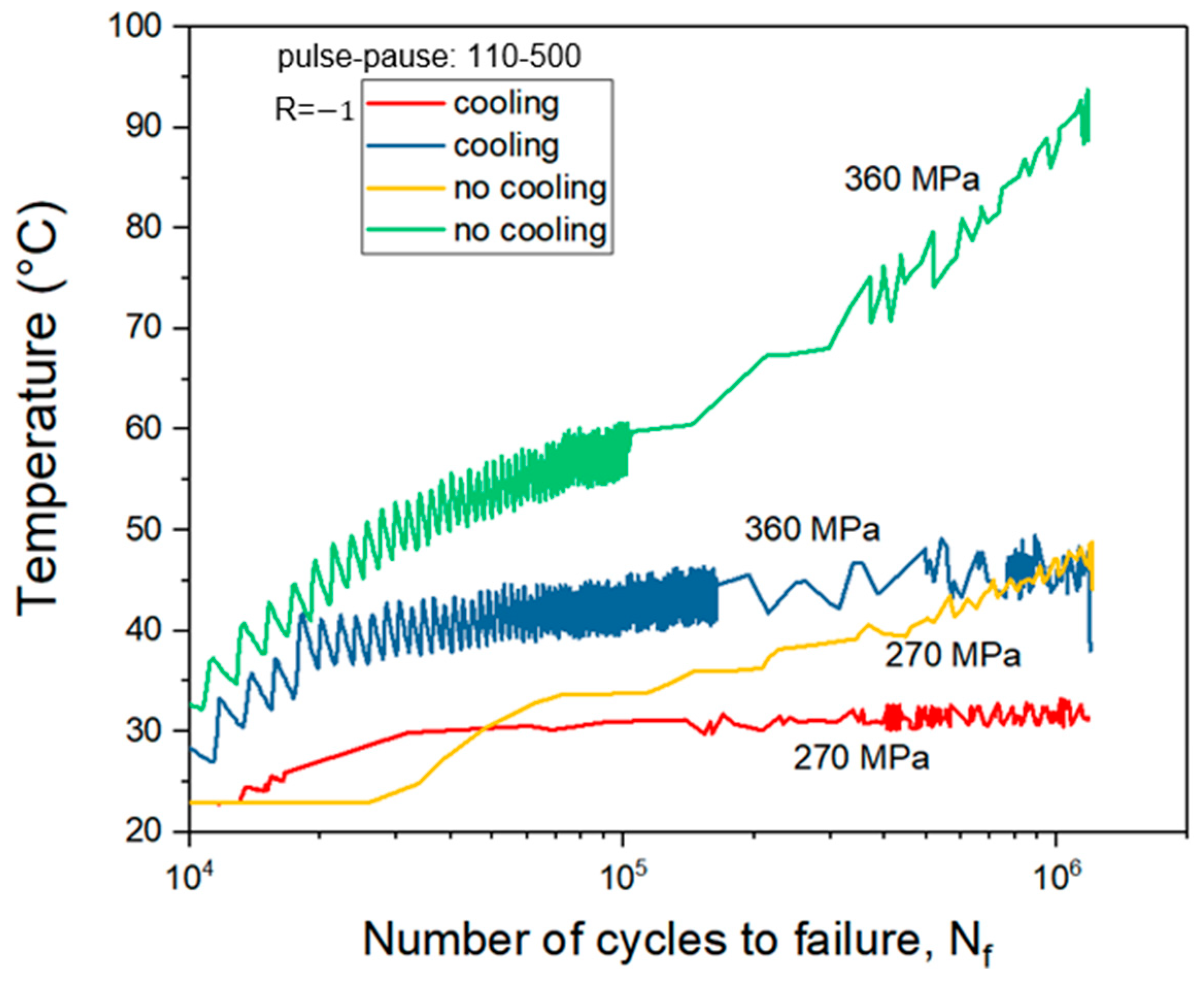
• A cooling system is essential for VHCF tests to manage high temperatures.
• Depending on the material studied, it may be necessary to increase pause times to maintain temperature control.
• An additional cooling mechanism may be required to keep the test at room temperature.

References

- Suresh, S. Fatigue of Materials; Cambridge University Press: New York, NY, USA, 1998. [Google Scholar]
- Downling, N.E. Mechanical Behavior of Materials: Engineering Methods for Deformation, Fracture, and Fatigue, 4th ed.; Pearson Education: Upper Saddle River, NJ, USA, 2012. [Google Scholar]
- Bathias, C.; Paris, P.C. Gigacycle Fatigue in Mechanical Practice; Informa UK Limited: London, UK, 2005. [Google Scholar]
- Bathias, C. There is no infinite fatigue life in metallic materials. Fatigue Fract. Eng. Mater Struct. 1999, 22, 559–565. [Google Scholar] [CrossRef]
- Kazymyrovych, V. Very high cycle fatigue of engineering materials: A literature review. Mater. Sci. Eng. 2009. [Google Scholar]
- Teixeira, M.C.; Brandão, A.L.T.; Parente, A.P.; Pereira, M.V. Artificial intelligence modeling of ultrasonic fatigue test to predict the temperature increase. Int. J. Fatigue 2022, 163, 106999. [Google Scholar] [CrossRef]
- Jeddi, D.; Palin-Luc, T. A review about the effects of structural and operational factors on the gigacycle fatigue of steels. Fatigue Fract. Eng. Mater Struct. 2018, 41, 969–990. [Google Scholar] [CrossRef]
- Crupi, V.; Epasto, G.; Guglielmino, E.; Risitano, G. Analysis of temperature and fracture surface of AISI4140 steel in very high cycle fatigue regime. Theor. Appl. Fract. Mech. 2015, 80, 22–30. [Google Scholar] [CrossRef]
- Peng, W.; Zhang, Y.; Qiu, B.; Xue, H. A Brief Review of the Application and Problems in Ultrasonic Fatigue Testing. AASRI Procedia 2012, 2, 127–133. [Google Scholar] [CrossRef]
- Ebara, R. The present situation and future problems in ultrasonic fatigue testing—Mainly reviewed on environmental effects and materials’ screening. Int. J. Fatigue 2006, 28, 1465–1470. [Google Scholar] [CrossRef]
- Peng, W.; Xue, H.; Ge, R.; Peng, Z. The influential factors on very high cycle fatigue testing results. MATEC Web Conf. 2018, 165, 20002. [Google Scholar]
- Lee, H.W.; Basaran, C. Predicting high cycle fatigue life with unified mechanics theory. Mech. Mater. 2022, 164, 104116. [Google Scholar] [CrossRef]
- Ellyin, F. Fatigue Damage, Crack Growth and Life Prediction; Springer Nature: Dordrecht, The Netherlands, 1996. [Google Scholar]
- Halford, G.R. The energy required for fatigue. J. Mater. 1966, 1, 3–18. [Google Scholar]
- Meneghetti, G.; Ricotta, M. The use of the specific heat loss to analyse the low and high cycle fatigue behavior of plain and notched specimens made of a stainless steel. Eng. Fract. Mech. 2012, 81, 2–16. [Google Scholar] [CrossRef]
- Amiri, M.; Khonsari, M.M. Introduction to Thermodynamics of Mechanical Fatigue; CRC Press: Boca Raton, FL, USA, 2013. [Google Scholar]
- Ricotta, M.; Meneghetti, G.; Atzori, B.; Risitano, G.; Risitano, A. Comparison of Experimental Thermal Methods for the Fatigue Limit Evaluation of a Stainless Steel. Metals 2019, 9, 677. [Google Scholar] [CrossRef]
- Meneghetti, G. Analysis of the fatigue strength of a stainless steel based on the energy dissipation. Int. J. Fatigue 2007, 29, 81–94. [Google Scholar] [CrossRef]
- Meneghetti, G.; Ricotta, M.; Atzori, B. A synthesis of the push-pull fatigue behavior of plain and notched stainless steel specimens by using the specific heat loss. Fatigue Fract. Eng. Mater Struct. 2013, 36, 1306–1322. [Google Scholar] [CrossRef]
- Amiri, M.; Khonsari, M.M. Rapid determination of fatigue failure based on temperature evolution: Fully reversed bending load. Int. J. Fatigue 2010, 32, 382–389. [Google Scholar] [CrossRef]
- Jiang, J.Y.; Khonsari, M.M. On the evaluation of fracture fatigue entropy. Theor. Appl. Fract. Mech. 2018, 96, 351–361. [Google Scholar] [CrossRef]
- Jiang, L.; Wang, H.; Liaw, P.K.; Brooks, C.R.; Klarstrom, D.L. Characterizartion of the temperatura evolution during high cycle fatigue. Metall. Mater. Trans. A 2001, 32, 2279–2296. [Google Scholar] [CrossRef]
- Fargione, G.; Geraci, A.; La Rosa, G.; Risitano, A. Rapid determination of the fatigue curve by thermographic method. Int. J. Fatigue 2002, 24, 11–19. [Google Scholar] [CrossRef]
- Sakai, T.; Nakagawa, A.; Oguma, N.; Nakamura, Y.; Ueno, A.; Kikuchi, S.; Sakaida, A. A review on fatigue fracture modes of structural metallic materials in very high cycle regime. Int. J. Fatigue 2016, 93, 339–351. [Google Scholar] [CrossRef]
- Wang, L.; Qian, X. Optimization-improved thermal–mechanical simulation of welding residual stresses in welded connections. Comput. Aided Civ. Infrastruct. Eng. 2024, 39, 1275–1293. [Google Scholar] [CrossRef]
- Wang, L.; Qian, X.; Feng, L. Effect of welding residual stresses on the fatigue life assessment of welded connections. Int. J. Fatigue 2024, 189, 108570. [Google Scholar] [CrossRef]
- Wang, L.; Qian, X. Welding residual stresses and their relaxation under cyclic loading in welded S550 steel plates. Int. J. Fatigue 2022, 162, 106992. [Google Scholar] [CrossRef]