

Mixed Convection Heat Transfer and Fluid Flow of Nanofluid/Porous Medium Under Magnetic Field Influence


Abstract
1. Introduction
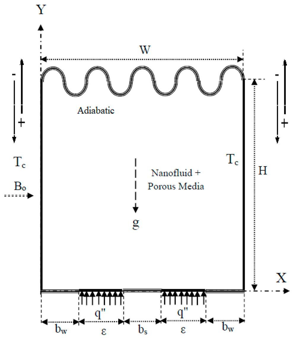
2. Problem Description
3. Mathematical Formulation
3.1. Assumptions
- The porous medium is homogeneous and isotropic.
- The nanofluid with a nanoparticle volume fraction ≤ 0.15 is Newtonian and incompressible.
- Laminar flow.
- Regular shape of the nanoparticles.
- Thermal equilibrium is assumed between the base fluid and the nanoparticles, along with no-slip conditions.
- The thermophysical properties of the nanofluid are fixed, except for variations in density that cause the body force term in the vertical component of the momentum equation (Equation (3)).
- A fixed and uniform magnetic field.
3.2. Distributions of the Velocity and Temperature
3.3. Streamfunction and Heatfunction
3.4. Entropy Generation
3.5. Boundary Conditions
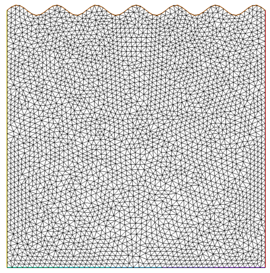
4. Numerical Method and Validation
5. Results and Discussion
- Case-1, where the isothermal vertical walls move from top to bottom ( = −1).
- Case-2, where the isothermal vertical walls move oppositely, the right wall moving from top to bottom ( = −1), and the left wall moving from bottom to top ( = 1).
- Case-3, where the isothermal vertical walls move from bottom to top ( = 1).
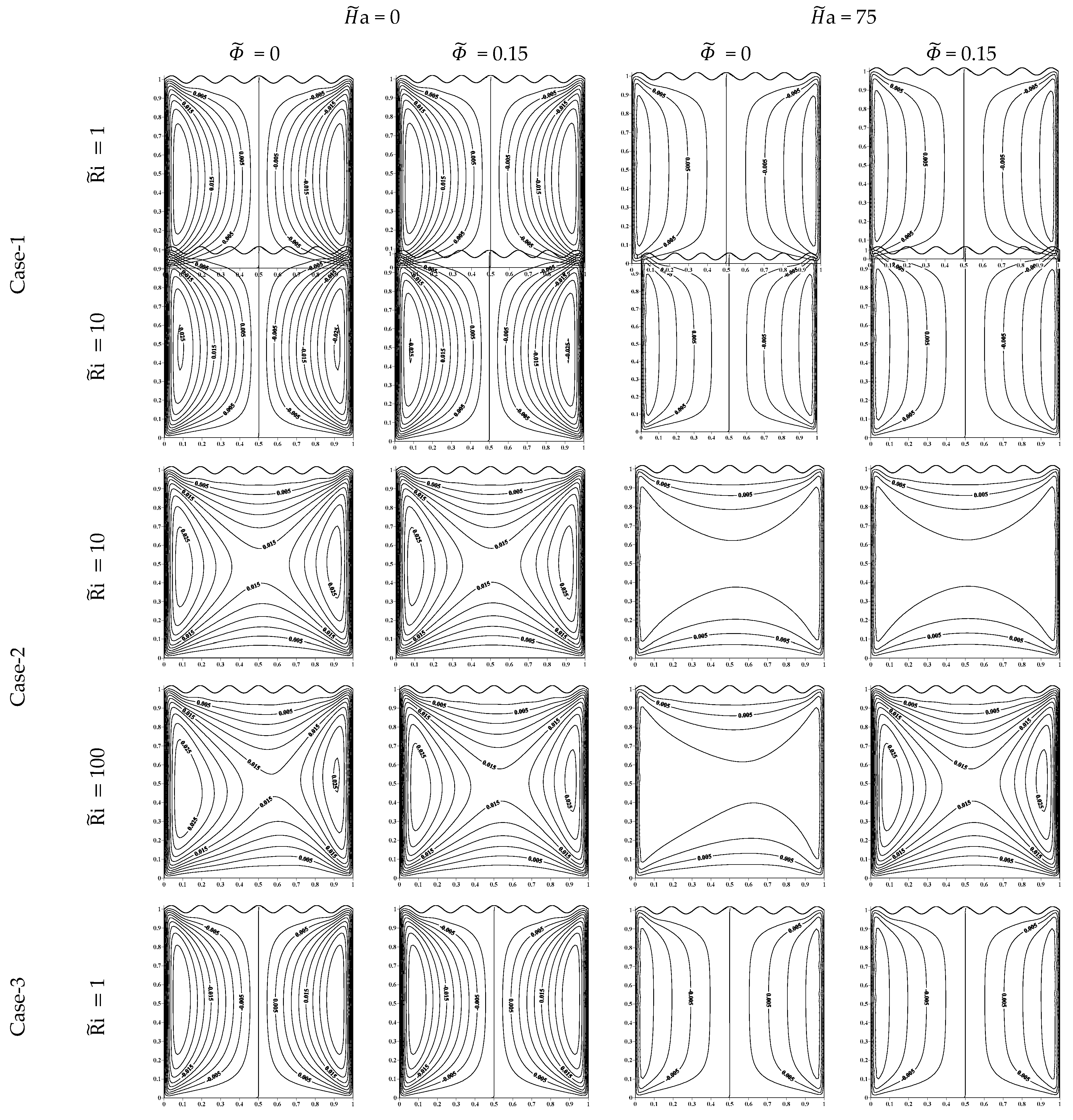
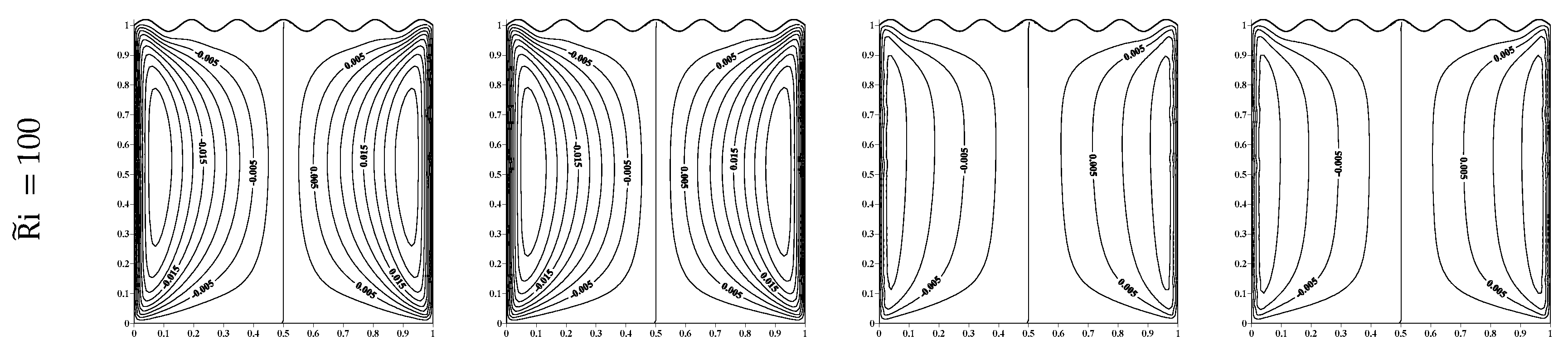
5.1. Streamfunction
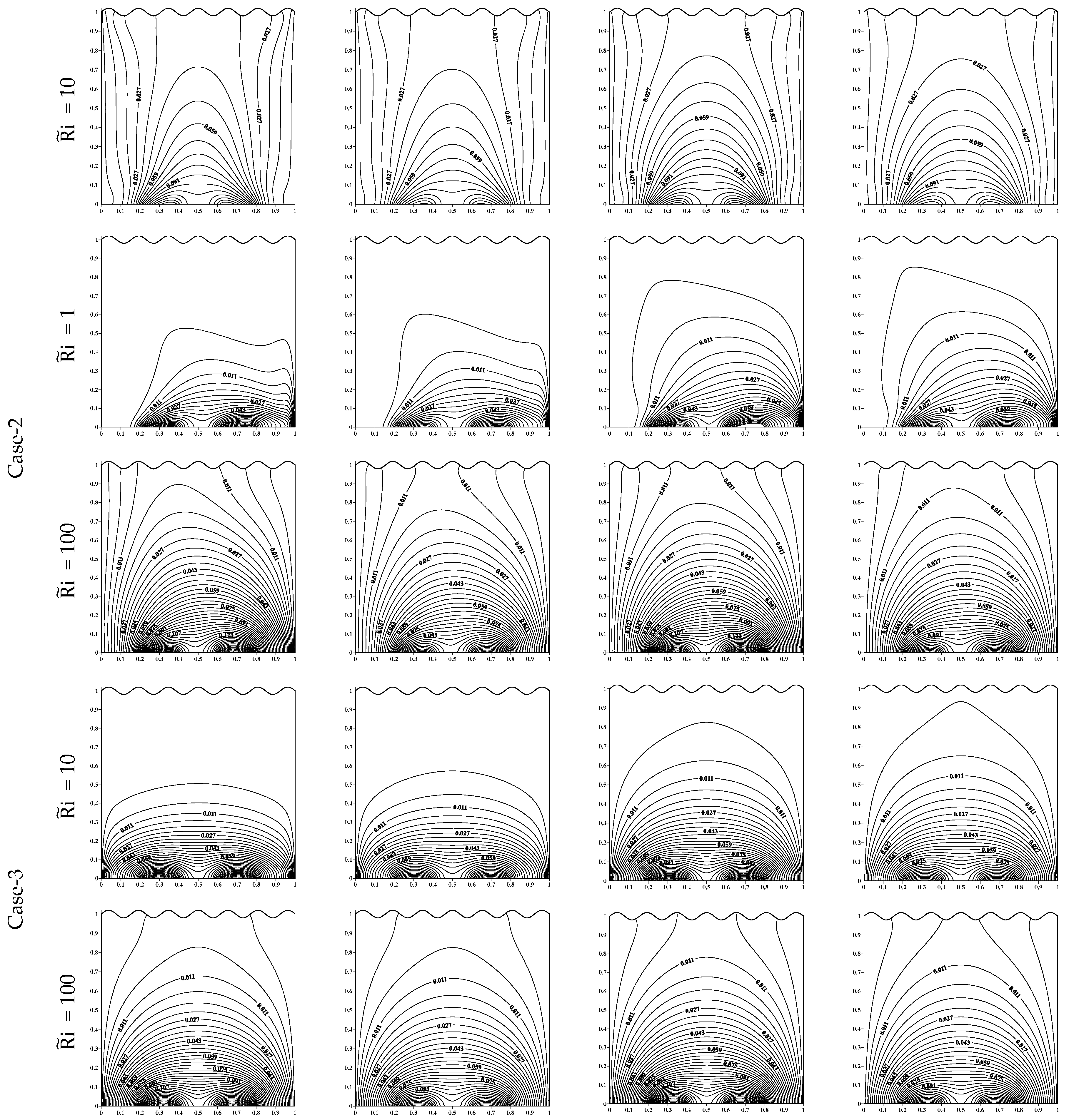
5.2. Isotherms
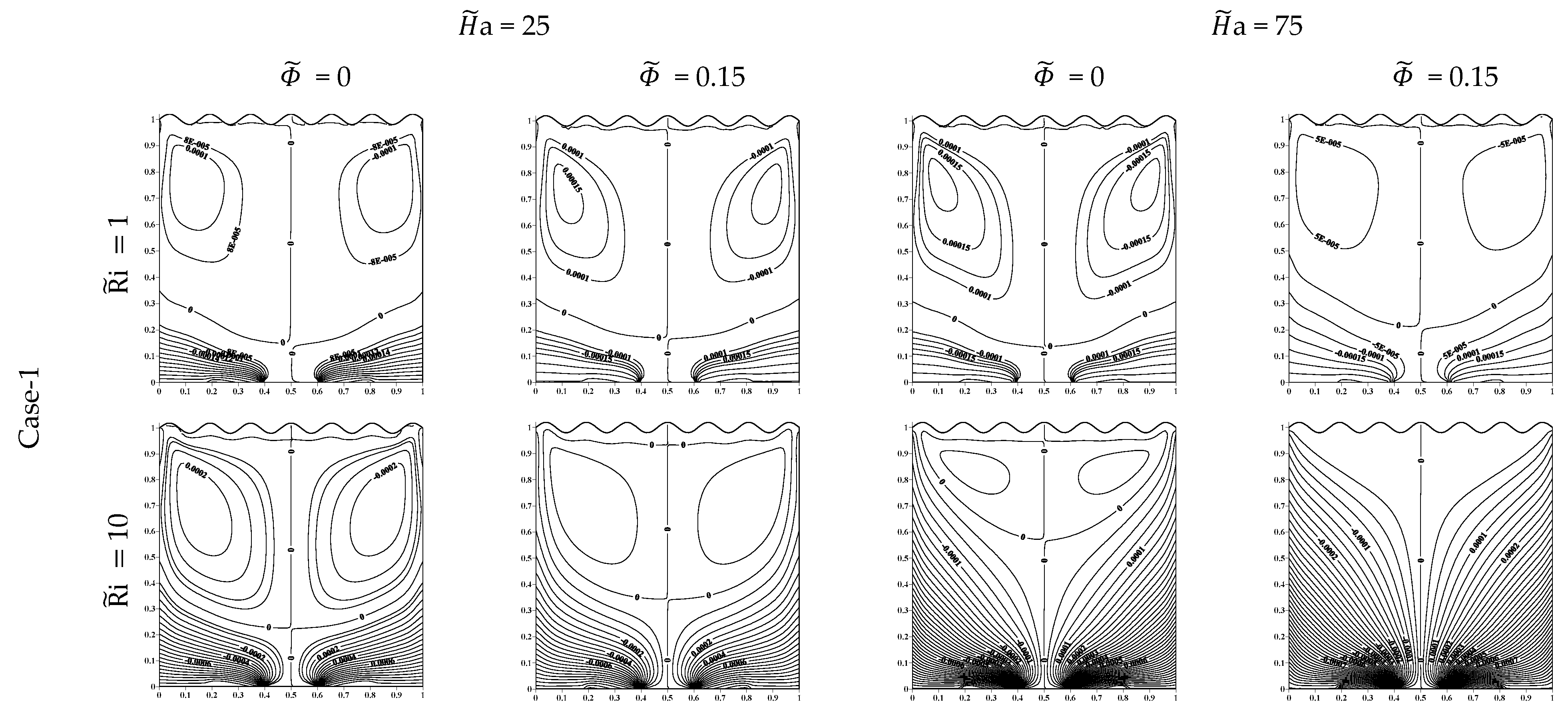
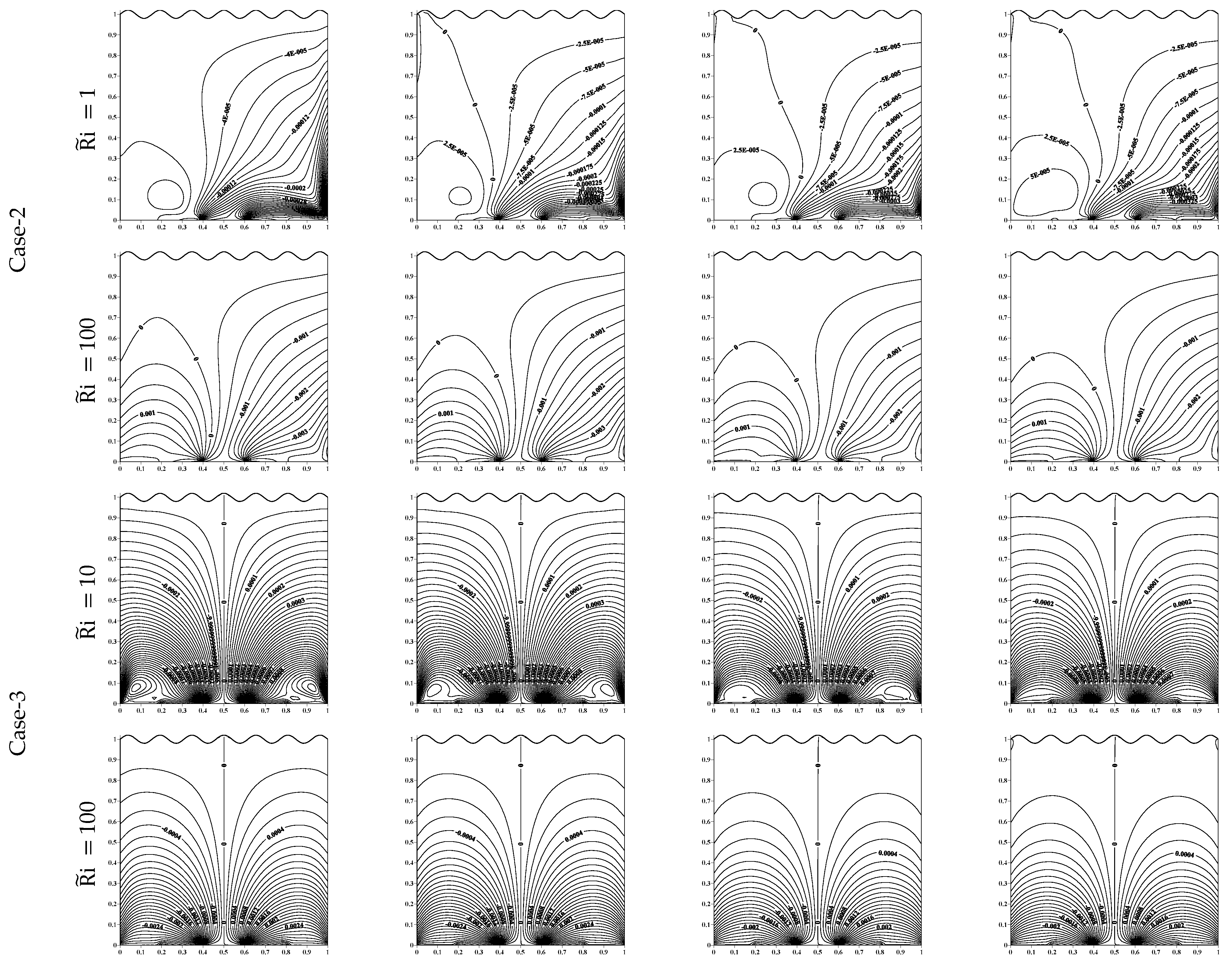
5.3. Heatfunction
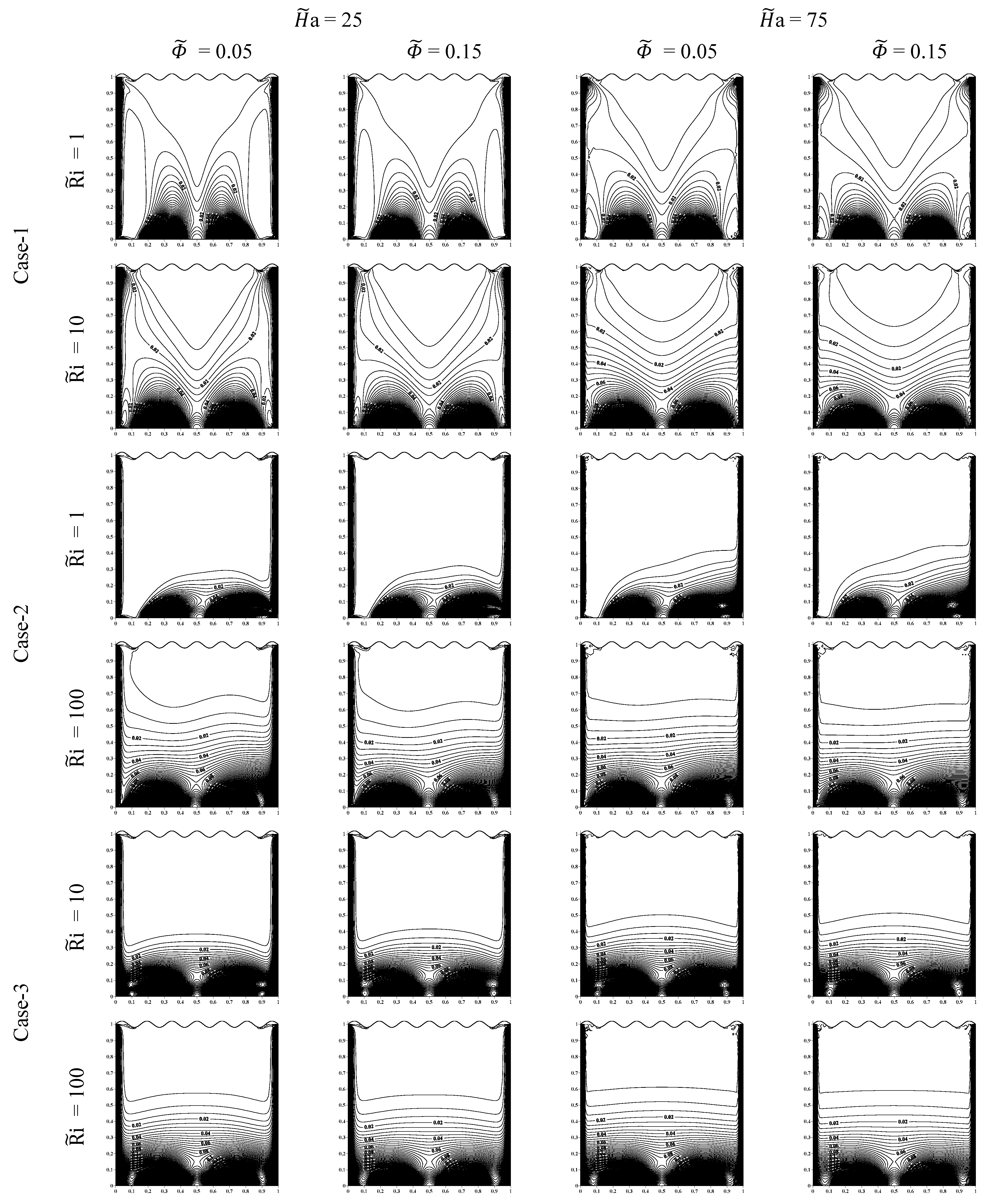
5.4. Entropy Generation
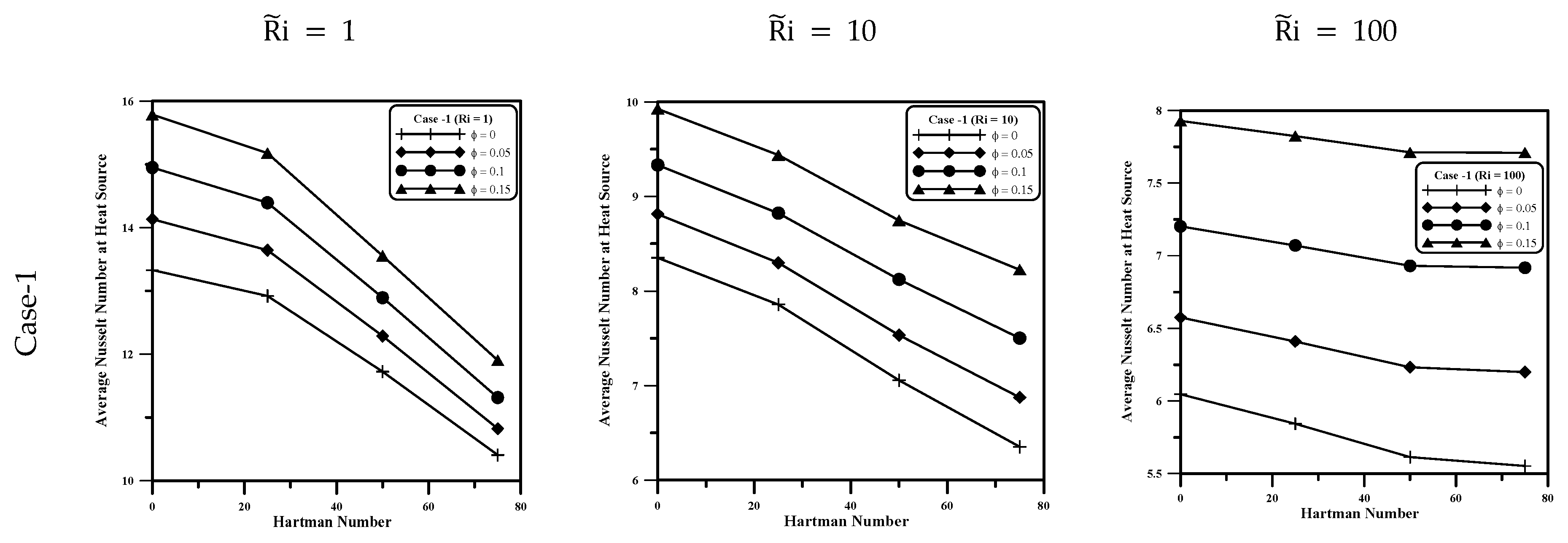
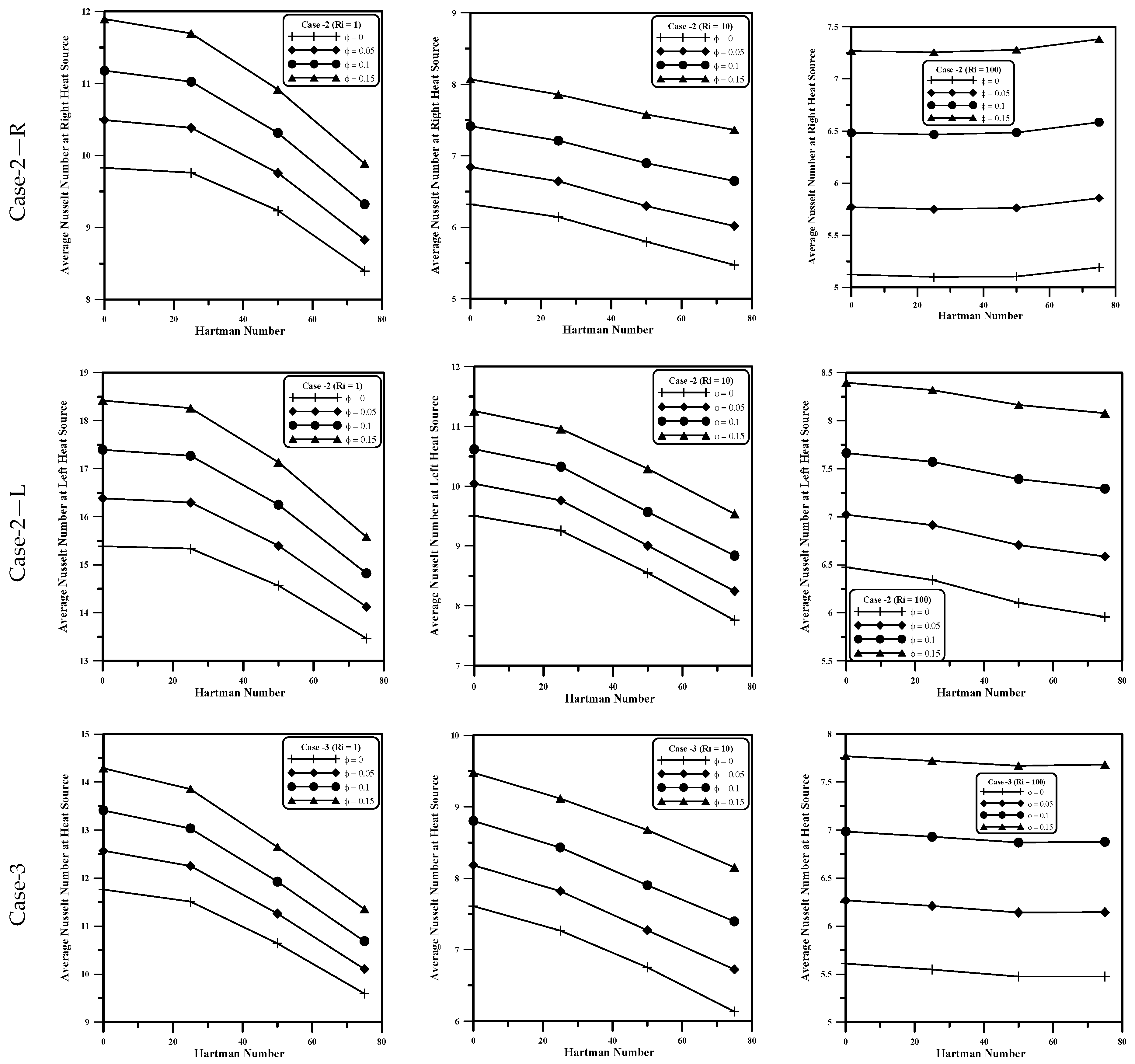
5.5. Average Nusselt Number at Hot Source
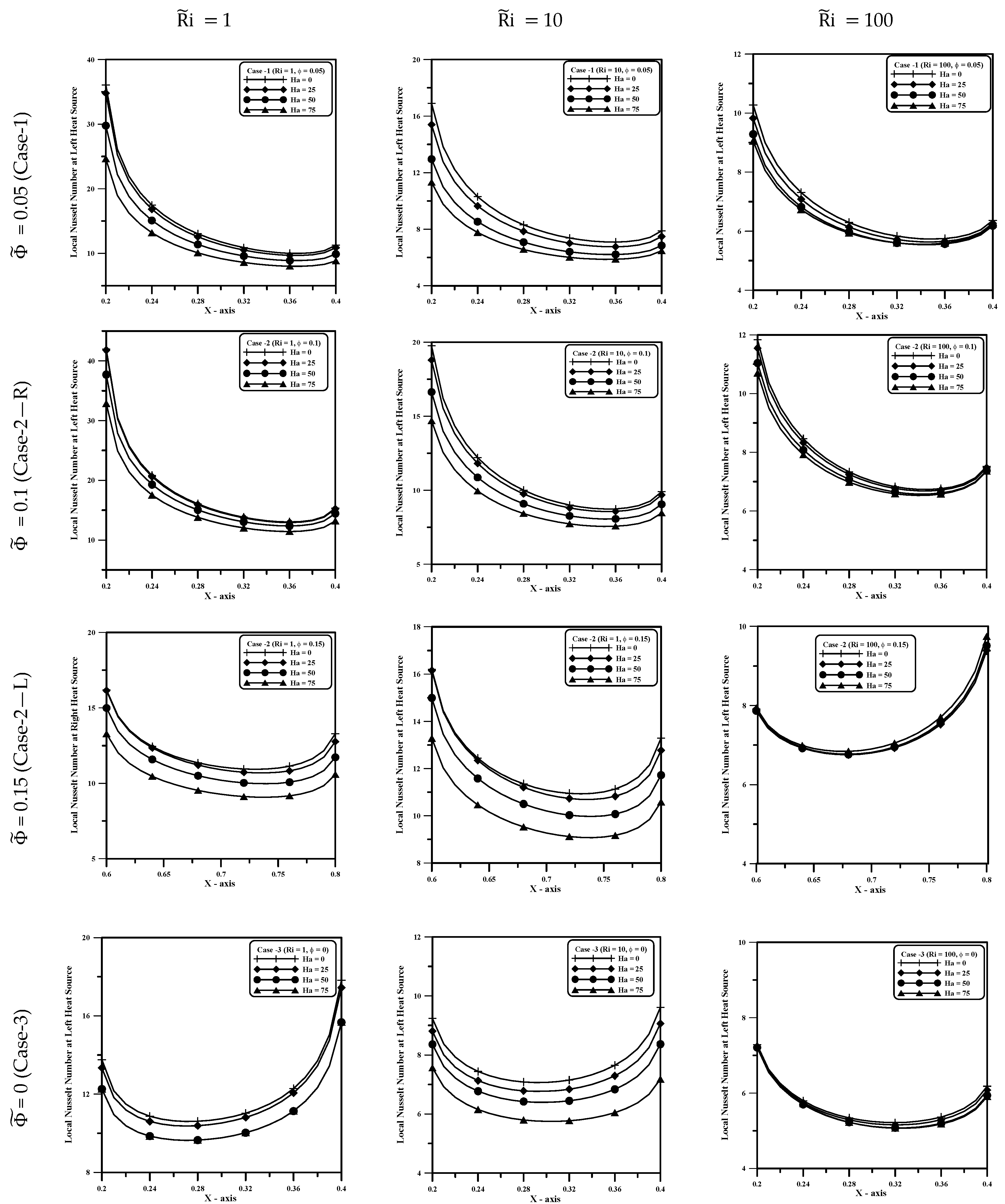
5.6. Local Nusselt Number
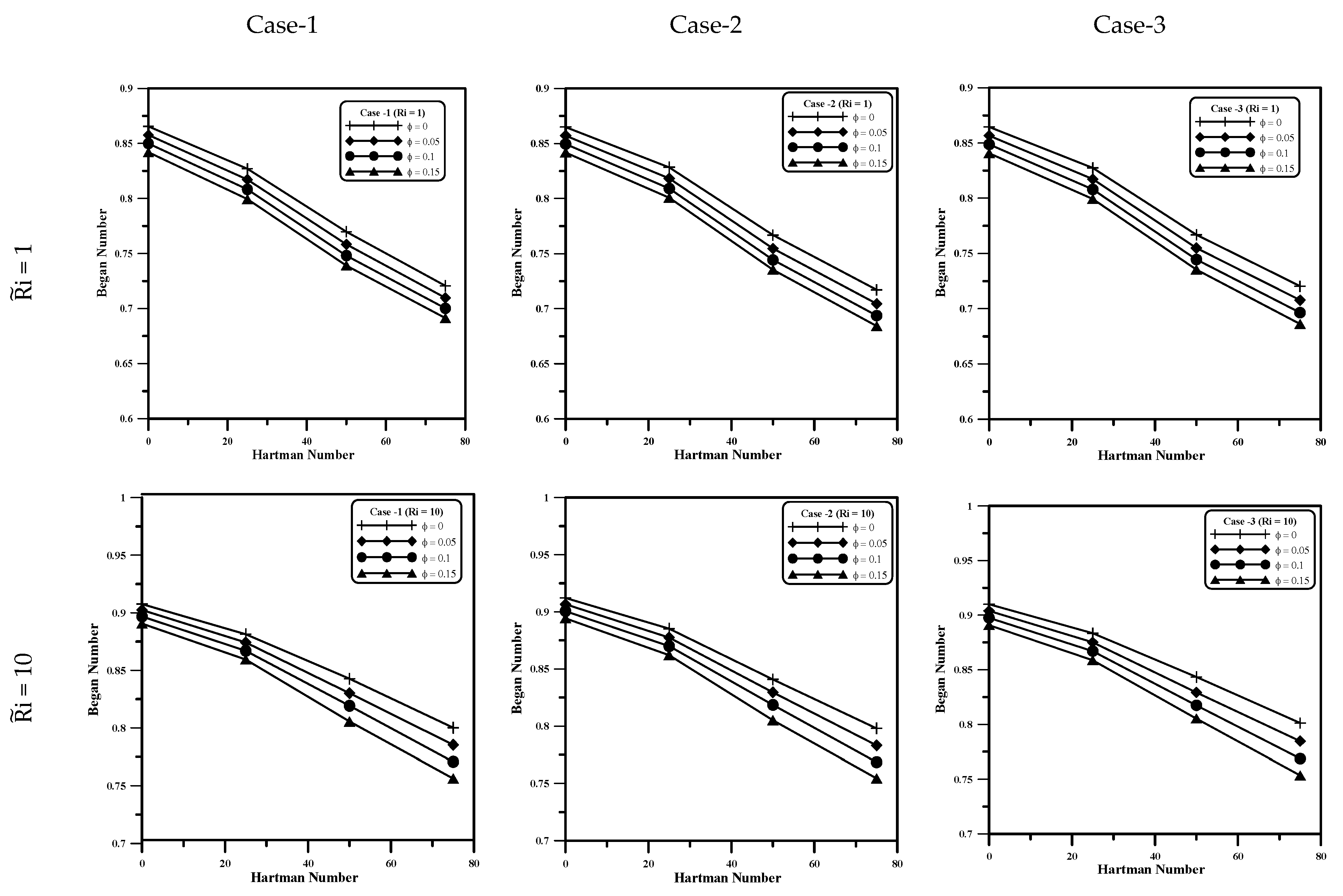
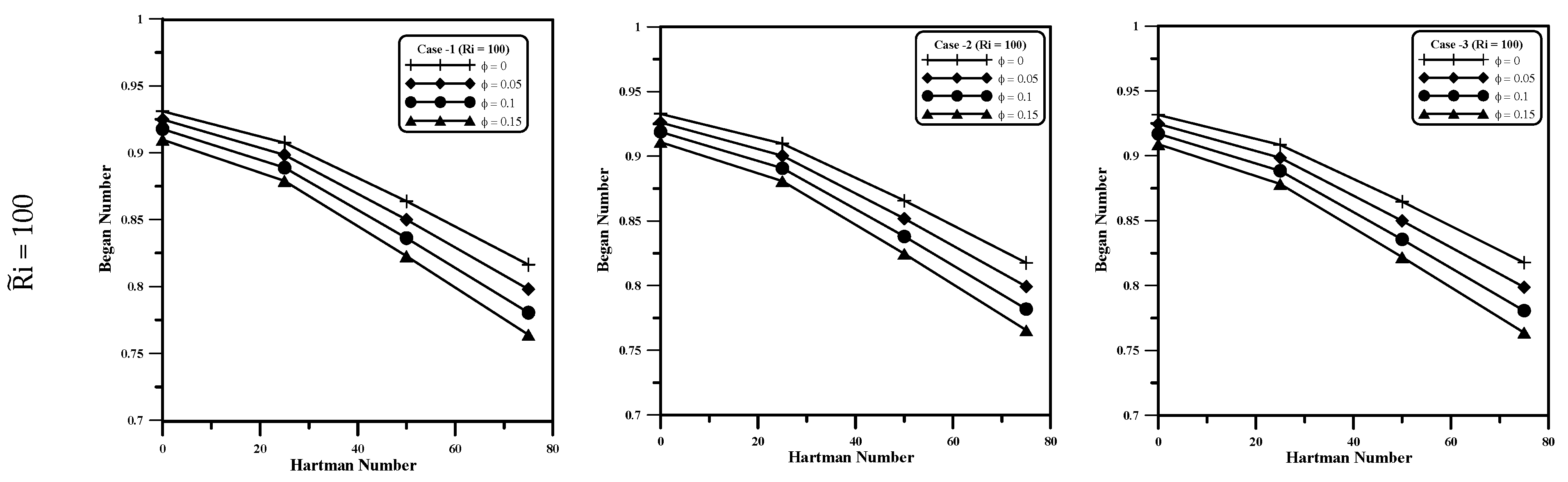
5.7. Bejan Number
6. Conclusions
- Case-3 is the most efficient scenario among others with similar physical parameters.
- The maximum streamfunction value decreases as a and increase, except for low where the maximum streamfunction increases as increases ( = 0.15).
- The increase in nanoparticle volume fraction will reduce the maximum temperature, and this reduction increases as a and increase.
- At low , circular heatlines appear at the top portion near the vertical wall, which has a negative sign (V = −1), and at the lower portion near the vertical wall, which has a positive sign (V = +1). These circular lines disappear at high .
- The dense entropy generation is located in the center and near the heat sources. At high values of = 100 and a, the entropy generation lines are distributed horizontally (parallel to the base wall) in the middle of the cavity.
- For all cases, the average number decreases as and a increase. The increase in the nanoparticle volume fraction inside the porous medium causes an increase in the average number and the rate of increment depends on the value of the .
- The local Nusselt number increases as and decrease, and a increases. The effect of on the local Nusselt number above the heat sources decreases at a high value of = 100.
- The e number decreases as and a increase. The effect of on the e increases significantly at high values of and a for all cases. The direction of the vertical wall movement (positive or negative) does not noticeably affect the e number. The variation of the average Number and e Number is linear with a for all volume fractions of nanoparticles.
Author Contributions
Funding
Institutional Review Board Statement
Informed Consent Statement
Data Availability Statement
Acknowledgments
Conflicts of Interest
Nomenclature
| o | magnetic field strength |
| e | Bejan number |
| bw, bs | Insulated wall dimensionless length at the bottom wall |
| p | Specific heat (kJ/kg·K) |
| a | Number of Darcy |
| r | Grashof number |
| Acceleration of gravity (m/s2) | |
| H | Enclosure height (m) |
| a | Hartmann number |
| Coefficient of thermal conductivity (W/m·K) | |
| c | Characteristic Length = W (m) |
| Local Nusselt number | |
| Average Nusselt number | |
| Dimensionless pressure | |
| Pressure (Pa) | |
| r | Prandtl number |
| ” | Heat flux (W/m2) |
| a | Number of Rayleigh |
| Richardson number (Gr/Re2) | |
| gen | Entropy generation |
| Temperature (K) | |
| X-direction dimensionless velocity component | |
| X-direction velocity component (m/s) | |
| Y-direction dimensionless velocity component | |
| Y-direction velocity component (m/s) | |
| W | enclosure Width (m) |
| Horizontal direction dimensionless coordinate | |
| Horizontal direction in cartesian coordinate (m) | |
| Vertical direction dimensionless coordinate | |
| Vertical direction in cartesian coordinate (m) | |
| Greek Symbols | |
| Thermal diffusivity (m2/s) | |
| Dimensionless temperature | |
| Dimensionless heat source length | |
| Dimensionless streamfunction | |
| Dynamic viscosity (kg·s/m) | |
| Kinematic viscosity (m2/s) | |
| volume fraction of nanoparticle | |
| Electrical conductivity | |
| Δ | Ref. temperature difference (°C) |
| Thermal expansion volumetric coefficient (K−1) | |
| Density (kg/m3) | |
| Dimensionless of heatfunction | |
| Subscripts | |
| c | Cold |
| f | Pure fluid |
| hf | at heat flux |
| max | Maximum |
| min | Minimum |
| nf | Nanofluid |
| p | Nanoparticles |
References
- Al-Zamily, A.M.J. Analysis of natural convection and entropy generation in a cavity filled with multi-layers of porous medium and nanofluid with a heat generation. Int. J. Heat Mass TranTransf. 2017, 106, 1218–1231. [Google Scholar] [CrossRef]
- Shah, S.S.; Haq, R.U.; Al-Kouz, W. Mixed convection analysis in a split lid-driven trapezoidal cavity having elliptic shaped obstacle. Int. Commun. Heat Mass Transf. 2021, 126, 105448. [Google Scholar] [CrossRef]
- Yeasmin, S.; Islam, Z.; Azad, A.; Alam, E.M.M.; Rahman, M.; Karim, M. Thermal performance of a hollow cylinder with low conductive materials in a lid-driven square cavity with partially cooled vertical wall. Ther. Sci. Eng. Prog. 2022, 35, 101454. [Google Scholar] [CrossRef]
- Sarker, S.; Alam, M.; Munshi, M. Modeling of Mixed Convection in a Lid Driven Wavy Enclosure with Two Square Blocks Placed at Different Positions. J. Appl. Math. Physics 2023, 11, 3984–3999. [Google Scholar] [CrossRef]
- Akhter, R.; Ali, M.M.; Alim, M.A. Magnetic field impact on double diffusive mixed convective hybrid-nanofluid flow and irreversibility in porous cavity with vertical wavy walls and rotating solid cylinder. Results Eng. 2023, 19, 101292. [Google Scholar] [CrossRef]
- Mahian, O.; Kolsi, L.; Amani, M.; Estellé, P.; Ahmadi, G.; Kleinstreuer, C.; Marshall, J.S.; Taylor, R.A.; Abu-Nada, E.; Rashidi, S.; et al. Recent advances in modeling and simulation of nanofluid flows—Part II. Appl. Phys. Rep. 2019, 791, 1–59. [Google Scholar] [CrossRef]
- Tian, X.; Gao, W.; Li, B.; Zhang, Z.; Leng, X. Mixed convection of nanofluid by two-phase model in an inclined cavity with variable aspect ratio. Chin. J. Phys. 2022, 77, 57–72. [Google Scholar] [CrossRef]
- Alsabery, A.I.; Abosinnee, A.S.; Al-Hadraawy, S.K.; Ismael, M.A.; Fteiti, M.A.; Hashim, I.; Sheremet, M.; Ghalambaz, M.; Chamkha, A.J. Convection heat transfer in enclosures with inner bodies: A review on single and two-phase nanofluid models. Renew. Sustain. Energy Rev. 2023, 183, 113424. [Google Scholar] [CrossRef]
- Colak, E.; Ekici, O.; Oztop, H.F. Mixed convection in a lid-driven cavity with partially heated porous block. Int. Commun. Heat Mass Transf. 2021, 126, 105450. [Google Scholar] [CrossRef]
- Shruti, B.; Dhinakaran, S. Lattice Boltzmann modeling of buoyant convection in an enclosure with differentially heated porous cylinders. Therm. Sci. Eng. Prog. 2024, 50, 102460. [Google Scholar] [CrossRef]
- Bouzennada, T.; Abderrahmane, A.; Aich, W.; Younis, O.; Ben Ali, N.; Kolsi, L. Heat transfer and fluid flow in nano-encapsulated PCM-filled undulated cavity. Ain Shams Eng. J. 2024, 15, 102669. [Google Scholar] [CrossRef]
- Devi, N.; Gnanasekaran, M.; Satheesh, A.; Kanna, P.; Taler, J.; Kumar, D.; Taler, D.; Sobota, T. Double-diffusive mixed convection in an inclined square cavity filled with nanofluid: A numerical study with external magnetic field and heated square blockage effects. Case Stud. Therm. Eng. 2024, 56, 104210. [Google Scholar] [CrossRef]
- Chattopadhyay, A. Exploring magnetohydrodynamic mixed convection in a complex chamber with hybrid nanoliquids: A numerical approach. Int. J. Therm. 2024, 22, 100629. [Google Scholar] [CrossRef]
- Bourantas, G.; Skouras, E.; Loukopoulos, V.; Burganos, V. Heat transfer and natural convection of nanofluids in porous media. Eur. J. Mech.-B/Fluids 2014, 43, 45–56. [Google Scholar] [CrossRef]
- Matin, M.H.; Ghanbari, B. Effects of Brownian Motion and Thermophoresis on the Mixed Convection of Nanofluid in a Porous Channel Including Flow Reversal. Trans. Porous Med. 2014, 101, 115–136. [Google Scholar] [CrossRef]
- Shuvo, M.S.; Hasib, M.H.; Saha, S. Entropy generation and characteristics of mixed convection in lid-driven trapezoidal tilted enclosure filled with nanofluid. Heliyon 2022, 8, e12079. [Google Scholar] [CrossRef]
- Moolya, S.; Satheesh, A. Role of magnetic field and cavity inclination on double diffusive mixed convection in rectangular enclosed domain. Int. Commun. Heat Mass Transf. 2020, 118, 104814. [Google Scholar] [CrossRef]
- Mondal, P.; Mahapatra, T.; Parveen, R. Entropy generation in nanofluid flow due to double diffusive MHD mixed convection. Heliyon 2021, 7, e06143. [Google Scholar] [CrossRef]
- Ibrahim, W.; Hirpho, M. Finite element analysis of mixed convection flow in a trapezoidal cavity with non-uniform temperature. Heliyon 2021, 7, e05933. [Google Scholar] [CrossRef]
- Akhter, R.; Ali, M.M.; Billah, M.M.; Uddin, M.N. Hybrid-nanofluid mixed convection in square cavity subjected to oriented magnetic field and multiple rotating rough cylinders. Results Eng. 2023, 18, 101100. [Google Scholar] [CrossRef]
- Ahmad, S.; Cham, B.M.; Liu, D.; Islam, S.U.; Hussien, M.A.; Waqas, H. Numerical analysis of heat and mass transfer of MHD natural convection flow in a cavity with effects of source and sink. Case Stud. Therm. Eng. 2024, 53, 103926. [Google Scholar] [CrossRef]
- Islam, S.; Islam, M.M.; Rana, B.M.J.; Islam, M.S.; Reza-E-Rabbi, S.; Hossain, M.S.; Rahman, M.M. Numerical investigation with sensitivity study of MHD mixed convective hexagonal heat exchanger using TiO2–H2O nanofluid. Res. Eng. 2023, 18, 101136. [Google Scholar] [CrossRef]
- Ahmed, S.E.; Raizah, Z.; Arafa, A.A.; Hussein, S.A. FEM treatments for MHD highly mixed convection flow within partially heated double-lid driven odd-shaped enclosures using ternary composition nanofluids. Int. Commun. Heat Mass Transf. 2023, 145, 106854. [Google Scholar] [CrossRef]
- Alomari, M.A.; Al-Farhany, K.; Al-Salami, Q.H.; Ali, I.R.; Biswas, N.; Mohamed, M.H.; Alqurashi, F. Numerical analysis to investigate the effect of a porous block on MHD mixed convection in a split lid-driven cavity with nanofluid. Int. J. Therm. 2024, 22, 100621. [Google Scholar] [CrossRef]
- Rajarathinam, M.; Akermi, M.; Khan, M.I.; Nithyadevi, N. MHD mixed convection heat transfer of copper water nanofluid in an inclined porous cavity having isothermal solid block. J. Magn. Magn. Mater. 2024, 593, 171845. [Google Scholar] [CrossRef]
- Mittal, N.; Manoj, V.; Kumar, D.S.; Satheesh, A. Numerical simulation of mixed convection in a porous medium filled with water/Al2O3 nanofluid. Heat Transf.—Asian Res. 2013, 42, 46–59. [Google Scholar] [CrossRef]
- Khorasanizadeh, H.; Nikfar, M.; Amani, J. Entropy generation of Cu–water nanofluid mixed convection in a cavity. Eur. J. Mech.-B/Fluids 2013, 37, 143–152. [Google Scholar] [CrossRef]
- Ahmed, S.E.; Mansour, M.; Mahdy, A. MHD mixed convection in an inclined lid-driven cavity with opposing thermal buoyancy force: Effect of non-uniform heating on both side walls. Nucl. Eng. Des. 2013, 265, 938–948. [Google Scholar] [CrossRef]
- Roy, M.; Biswal, P.; Roy, S.; Basak, T. Heat flow visualization during mixed convection within entrapped porous triangular cavities with moving horizontal walls via heatline analysis. Int. J. Heat Mass Transf. 2017, 108, 468–489. [Google Scholar] [CrossRef]
- Al-Khaleel, M.; Abderrahmane, A.; Younis, O.; Jamshed, W.; Guedri, K.; Safdar, R.; Tag, S.M. A Galerkin finite element-based study of MHD mixed convective of Ostwald-de Waele nanofluids in a lid-driven wavy chamber. Res. Phy. 2024, 5, 107232. [Google Scholar] [CrossRef]
- Abedallh, A.S.; Alomar, O.R.; Yasin, N.J. Numerical and experimental investigation on mixed convection heat transfer inside cavity heated from below with reciprocating moving upper surface. Int. Commun. Heat Mass Transf. 2024, 159, 108242. [Google Scholar] [CrossRef]
- Biswal, P.; Basak, T. Sensitivity of heatfunction boundary conditions on invariance of Bejan’s heatlines for natural convection in enclosures with various wall heatings. Int. J. Heat Mass Transf. 2015, 89, 1342–1368. [Google Scholar] [CrossRef]


| Properties | Pure Water | Titanium Oxide (TiO2) |
|---|---|---|
| (J/kg·K) | 4179 | 686.2 |
| (W/m.K) | 0.613 | 8.953 |
| (kg/m3) | 997.1 | 4250 |
| (1/K) × 105 | 21 | 0.9 |
| Σ (Ω·m)−1 | 0.05 | 3.7 × 10³ |
| (pa·s) | 0.00091 | |
| r | 6.2 |
| Elements | Grid | |max| | max | |
|---|---|---|---|---|
| 2052 | 30 × 30 | 0.056116 | 0.065968 | 17.1827 |
| 3809 | 40 × 40 | 0.056445 | 0.065017 | 17.4335 |
| 6023 | 50 × 50 | 0.056495 | 0.064776 | 17.5001 |
| 8930 | 60 × 60 | 0.056508 | 0.064404 | 17.5406 |
| 12,226 | 70 × 70 | 0.056511 | 0.064304 | 17.5570 |
| 15,993 | 80 × 80 | 0.056510 | 0.064300 | 17.5590 |
| a | r = 100 | r = 10,000 | ||||
|---|---|---|---|---|---|---|
| Ref. | Present | Ref. | Present | Ref. | Present | |
| = 0% | = 0% | = 5% | = 5% | = 2% | = 2% | |
| 0.001 | 1.0020 | 1.0017 | 1.1520 | 1.1520 | 1.4300 | 1.4000 |
| 0.01 | 1.0060 | 1.0055 | 1.1550 | 1.1560 | 2.5140 | 2.4000 |
| 0.1 | 1.0060 | 1.0059 | 1.1580 | 1.1590 | 2.8500 | 2.8000 |
| a | e | ||||
|---|---|---|---|---|---|
| Ref. | Present | ||||
| 105 | 1 | 0 | 0.0001 | 5.200 | 5.100 |
| 105 | 100 | 0.05 | 0.0001 | 9.700 | 9.560 |
| 104 | 10 | 0.05 | 0.0001 | 4.000 | 3.950 |
| e | r | Ref. | Present |
|---|---|---|---|
| 50 | 104 | 0.110 | 0.115 |
| 100 | 103 | 0.097 | 0.102 |
| 250 | 104 | 0.108 | 0.113 |
| 500 | 105 | 0.135 | 0.139 |
| i | Ref. | Present |
|---|---|---|
| 1 | 2 | 2.11 |
| 10 | 2.875 | 2.92 |
| = 0.05 | = 0.1 | = 0.15 | ||
| = 1 | a = 0 | −0.0377 | −0.0683 | −0.0919 |
| a = 25 | −0.3975 | −0.3625 | 0.0413 | |
| a = 50 | −0.7548 | −0.6533 | 0.1814 | |
| a = 75 | −0.9180 | −0.7908 | 0.2335 | |
| = 100 | a = 0 | −1.9115 | −3.3081 | −4.3558 |
| a = 25 | −1.8495 | −2.8556 | −3.1980 | |
| = 0.05 | = 0.1 | = 0.15 | ||
| 1 | a = 25 | −0.3475 | −0.2911 | 0.1095 |
| a = 75 | −0.9306 | −0.7790 | 0.3023 | |
| 10 | a = 0 | −0.1130 | −0.2203 | −0.3216 |
| a = 50 | −0.8070 | −0.7646 | 1.2492 | |
| 100 | a = 0 | −1.4046 | −2.4334 | −3.2035 |
| a = 75 | −1.2811 | −1.3874 | −0.5031 | |
| = 0.05 | = 0.1 | = 0.15 | ||
| 1 | a = 0 | −0.0076 | −0.0105 | −0.0093 |
| a = 75 | −0.8915 | −0.7368 | 0.3146 | |
| 100 | a = 0 | −0.3534 | −0.6851 | −0.9711 |
| a = 50 | −0.5563 | −0.2997 | −0.6740 | |
| = 0.05 | = 0.1 | = 0.15 | ||
| = 1 | a = 25 | −7.0116 | −13.415 | −19.2531 |
| a = 75 | −6.1149 | −12.1202 | −18.0556 | |
| = 10 | a = 0 | −6.9715 | −13.613 | −19.96 |
| a = 75 | −8.9113 | −17.393 | −25.285 | |
| = 100 | a = 25 | −9.823 | −18.902 | −27.109 |
| a = 50 | −10.602 | −20.017 | −28.379 | |
| = 0.05 | = 0.1 | = 0.15 | ||
| 1 | a = 25 | −6.3891 | −12.227 | −17.634 |
| a = 75 | −5.5019 | −11.008 | −16.57 | |
| 10 | a = 0 | −7.8314 | −15.135 | −22.155 |
| a = 75 | −9.1976 | −17.813 | −25.79 | |
| 100 | a = 0 | −11.144 | −20.828 | −29.298 |
| a = 50 | −11.314 | −21.105 | −29.637 | |
| = 0.05 | = 0.1 | = 0.15 | ||
| 1 | a = 0 | −6.8709 | −13.0376 | −18.6837 |
| a = 75 | −5.6269 | −11.1926 | −16.7592 | |
| 10 | a = 25 | −7.2647 | −14.1153 | −20.6392 |
| a = 75 | −8.7446 | −16.9719 | −24.6290 | |
| 100 | a = 0 | −10.4928 | −19.6325 | −27.6950 |
| a = 50 | −10.8242 | −20.2358 | −28.4800 | |
| = 0.05 | = 0.1 | = 0.15 | = 0.05 | = 0.1 | = 0.15 | |||
|---|---|---|---|---|---|---|---|---|
| Case-1 | Case-2—R | |||||||
| 1 | a = 0 | 6.0314 | 12.1656 | 18.4543 | a = 50 | 5.7124 | 11.5635 | 17.6364 |
| a = 75 | 3.9877 | 8.7239 | 14.3719 | a = 75 | 4.8852 | 10.0608 | 15.6804 | |
| 10 | a = 25 | 5.6283 | 12.2966 | 20.1092 | a = 0 | 5.6416 | 11.7158 | 18.4518 |
| a = 75 | 8.2621 | 18.1148 | 29.5096 | a = 75 | 6.2869 | 13.9295 | 22.9128 | |
| 100 | a = 0 | 8.7163 | 19.1010 | 31.0973 | a = 0 | 8.4530 | 18.3633 | 29.6857 |
| a = 75 | 11.6315 | 24.5817 | 38.8383 | a = 25 | 8.9660 | 19.3598 | 31.1549 | |
| Case-2—L | Case-3 | |||||||
| 1 | a = 25 | 6.3846 | 12.9623 | 19.8239 | a = 0 | 6.8837 | 14.0251 | 21.4829 |
| a = 75 | 5.1647 | 11.0236 | 17.7445 | a = 25 | 6.4682 | 13.2405 | 20.3778 | |
| 10 | a = 0 | 8.1944 | 17.2683 | 27.6383 | a = 50 | 4.6370 | 13.8467 | 29.4897 |
| a = 50 | 8.1840 | 18.4074 | 34.2044 | a = 75 | 9.6157 | 20.5602 | 32.9092 | |
| 100 | a = 0 | 12.6280 | 26.5325 | 41.8510 | a = 25 | 11.9096 | 24.9062 | 39.1550 |
| a = 75 | 12.7955 | 26.8032 | 42.1463 | a = 75 | 12.2510 | 25.6390 | 40.3154 | |
| Case-1 | Case-2 | Case-3 | ||||||||||
|---|---|---|---|---|---|---|---|---|---|---|---|---|
| a | 0.05 | 0.1 | 0.15 | a | 0.05 | 0.1 | 0.15 | a | 0.05 | 0.1 | 0.15 | |
| 1 | 0 | −0.8992 | −1.8001 | −2.7056 | 25 | −1.2219 | −2.3261 | −3.3334 | 0 | −0.9124 | −1.8318 | −2.7604 |
| 75 | −1.5221 | −2.8467 | −4.0660 | 50 | −1.5953 | −2.9474 | −4.0988 | 25 | −1.2233 | −2.3478 | −3.3861 | |
| 10 | 0 | −0.5726 | −1.1814 | −1.8679 | 25 | −0.8619 | −1.7249 | −2.6050 | 50 | −0.5618 | −1.9784 | −4.6275 |
| 50 | −0.2965 | −1.6199 | −5.0097 | 75 | −1.8668 | −3.6994 | −5.4666 | 75 | −2.0629 | −4.0507 | −5.9542 | |
| 100 | 25 | −0.9887 | −2.0359 | −3.1259 | 0 | −0.7114 | −1.4946 | −2.3495 | 0 | −0.7597 | −1.5718 | −2.4445 |
| 75 | −2.2338 | −4.3877 | −6.4092 | 25 | −1.0315 | −2.0949 | −3.1847 | 75 | −2.3306 | −4.5329 | −6.6013 | |
Disclaimer/Publisher’s Note: The statements, opinions and data contained in all publications are solely those of the individual author(s) and contributor(s) and not of MDPI and/or the editor(s). MDPI and/or the editor(s) disclaim responsibility for any injury to people or property resulting from any ideas, methods, instructions or products referred to in the content. |
© 2025 by the authors. Licensee MDPI, Basel, Switzerland. This article is an open access article distributed under the terms and conditions of the Creative Commons Attribution (CC BY) license (https://creativecommons.org/licenses/by/4.0/).
Share and Cite
Al-Kaby, R.N.; Abdulhaleem, S.M.; Hameed, R.H.; Yasiry, A. Mixed Convection Heat Transfer and Fluid Flow of Nanofluid/Porous Medium Under Magnetic Field Influence. Appl. Sci. 2025, 15, 1087. https://doi.org/10.3390/app15031087
Al-Kaby RN, Abdulhaleem SM, Hameed RH, Yasiry A. Mixed Convection Heat Transfer and Fluid Flow of Nanofluid/Porous Medium Under Magnetic Field Influence. Applied Sciences. 2025; 15(3):1087. https://doi.org/10.3390/app15031087
Chicago/Turabian StyleAl-Kaby, Rehab N., Samer M. Abdulhaleem, Rafel H. Hameed, and Ahmed Yasiry. 2025. "Mixed Convection Heat Transfer and Fluid Flow of Nanofluid/Porous Medium Under Magnetic Field Influence" Applied Sciences 15, no. 3: 1087. https://doi.org/10.3390/app15031087
APA StyleAl-Kaby, R. N., Abdulhaleem, S. M., Hameed, R. H., & Yasiry, A. (2025). Mixed Convection Heat Transfer and Fluid Flow of Nanofluid/Porous Medium Under Magnetic Field Influence. Applied Sciences, 15(3), 1087. https://doi.org/10.3390/app15031087