Abstract
This study presents six degrees of freedom (6-DoF) pose estimation of an object from a single RGB image and retrieval of the matching CAD model by measuring the similarity between RGB and CAD rendering images. The 6-DoF pose estimation of an RGB object is one of the important techniques in 3D computer vision. However, in addition to 6-DoF pose estimation, retrieval and alignment of the matching CAD model with the RGB object should be performed for various industrial applications such as eXtended Reality (XR), Augmented Reality (AR), robot’s pick and place, and so on. This paper addresses 6-DoF pose estimation and CAD model retrieval problems simultaneously and quantitatively analyzes how much the 6-DoF pose estimation affects the CAD model retrieval performance. This study consists of two main steps. The first step is 6-DoF pose estimation based on the PoseContrast network. We enhance the structure of PoseConstrast by adding variance uncertainty weight and feature attention modules. The second step is the retrieval of the matching CAD model by an image similarity measurement between the CAD rendering and the RGB object. In our experiments, we used 2000 RGB images collected from Google and Bing search engines and 100 CAD models from ShapeNetCore. The Pascal3D+ dataset is used to train the pose estimation network and DELF features are used for the similarity measurement. Comprehensive ablation studies about the proposed network show the quantitative performance analysis with respect to the baseline model. Experimental results show that the pose estimation performance has a positive correlation with the CAD retrieval performance.
1. Introduction
In 3D computer vision, 6-DoF (degrees of freedom) pose estimation is a study of finding the 3D position and 3D orientation of a real object in images or videos. Precise knowledge of the object’s 6-DoF pose with respect to the camera coordinate system enhances the performance in various applications such as eXtended Reality (XR), Augmented Reality (AR), robotic pick and place, autonomous vehicle, etc. In the studies of robotic pick and place, precise pose estimation is essential for picking up objects using camera images. The complete pose information of an object can be effectively used even when the object is partially occluded. In the studies of autonomous vehicles, estimating the pose of surrounding objects is necessary for recognizing the environment and obstacles, thereby enabling stable and safe driving [1].
For XR and AR applications, 6-DoF pose estimation of real objects is necessary to precisely align graphic models with the objects in the image space. A graphic model, such as a CAD model in the world coordinate system, should be transformed and projected to the image plane of the camera so that the projection of the CAD model is precisely aligned with the object area. Especially for XR and AR applications, the shape-matching model with the real object should be retrieved from a CAD model database before aligning the CAD model with the object in the image space. Therefore, not only the pose estimation of an RGB object but also the CAD model retrieval problem should be addressed simultaneously to align the RGB real object and CAD model exactly.
Conventional computer vision methods for estimating 6-DoF pose involve extracting and matching image features. Well-known image features include Scale-Invariant Feature Transform (SIFT) [2], Speeded Up Robust Features (SURF) [3], Oriented FAST and Rotated BRIEF (ORB) [4], and so on. Conventional feature-based 6-DoF pose estimation methods face limitations when the number of extracted features is small or when an object is placed with a complex background due to high sensitivity to data quality and outliers. Other 6-DoF methods include Iterative Closest Point (ICP) [5] and Perspective-n-Point (PnP) algorithm [6]. ICP estimates correspondences between different point clouds to find rotation and translation transformations, and PnP estimates object pose using the perspective projections between 3D points and corresponding 2D image points.
Recent advances in deep learning techniques and the availability of big data have overcome some limitations of traditional feature-based methods. In addition to RGB images, 3D data from depth cameras, such as RGB-D and point clouds, have been utilized. Several approaches have been developed to estimate the 6-DoF pose of objects using deep learning methods. PoseCNN [7] and Deep-6DPose [8] employ convolutional neural networks (CNNs) for regression-based pose estimation. PoseNet [9] and PPR-Net [10] use point clouds as input data for pose estimation, while DenseFusion [11] combines various data types to extract comprehensive information for accurate pose estimation. Furthermore, methods such as Dpod [12] and Rnnpose [13] utilize deep learning networks to predict object pose even when parts of the object are occluded. These advancements highlight the capability of deep learning networks to estimate object pose more accurately, even in the presence of various obstacles.
The 3D CAD model retrieval problem is to search for a CAD model from CAD datasets, which is the best matching with an input RGB object. Conventional CAD retrieval methods mostly address the search for matching CAD models from RGB or RGB-D images [14]. However, there are few studies of simultaneous searching for the best CAD model and estimating the 6-DoF pose of an input RGB image [15,16]. Park et al. [15] and Gümeli C. et al. [16] introduced frameworks similar to the proposed method. These methods detect an RGB object from an input image, estimate the 4-DoF or 6-DoF pose, and search the matching CAD model. Because each problem of 6-DoF pose estimation and CAD model retrieval from an input RGB is inherently not easy, simultaneous pose estimation and CAD model retrieval has not been commonly addressed.
In this study, we propose a combined method of simultaneous 6-DoF pose estimation and CAD model retrieval from a single RGB image. From the single RGB image, we detect a real object and estimate the rotational and translational transformation of the object from the reference CAD to the camera coordinate systems. Then, the best-matching CAD model is retrieved from a dataset by the proposed similarity measurement between RGB and rendered CAD images.
Our contributions are twofold, and the summary of the proposed methods is as follows. First, for 6-DoF pose estimation, we employ “PoseContrast: Class-Agnostic Object Viewpoint Estimation in the Wild with the Pose-Aware Contrastive Learning” (PoseContrast) [17] as the baseline model. PoseConstrast estimates the 3-DoF rotational pose of an object regardless of the object classes. In the original PoseContrast, the number of public datasets for pose estimation is relatively small compared to those used for other tasks [18]. Therefore, using PoseContrast as the baseline model is advantageous since it is based on contrastive learning. In the proposed pose estimation network, we add new modules to the baseline to generate attention weights, which are used to update the feature output from the network rather than using features extracted by the multilayer perceptron (MLP) of the baseline network.
Subsequently, several network modules are added to increase the attention weights of the important parts of the features. To do this, the probability variance of each 3-DoF rotational angle is estimated, and the attention weights to meaningful aspects of the features are refined. Then, the refined features are used as inputs for the MLP. Additionally, we enhance the network’s performance by utilizing a loss function based on quaternion.
Second, we propose a CAD model retrieval method to determine the best matching CAD model with the RGB object. The CAD model retrieval is based on deep features by “Large-Scale Image Retrieval with Attentive Deep Local Features” (DELF) [19], which has been introduced to find the 2D affine transformation between images. For the retrieval experiment, we select ten CAD candidates in each object class. Using the pose estimation result, all candidates are transformed to the camera coordinate system, and 2D projections are rendered. Then, image similarity between the candidates and the RGB object is measured to determine the best matching model.
Therefore, the image similarity between the rendered CAD model and the RGB object is directly related to the pose estimation result. The better the pose of the RGB object is estimated, the more the image similarity between the matching CAD model and the RGB object is increased. To evaluate this correlation, we propose a correlation measurement between the two performances of pose estimation and CAD retrieval. The experimental results show that there is a positive correlation between the two performances.
The architecture of the proposed method is shown in Figure 1 and it can be summarized as follows. First, an RGB object is detected and segmented from a single RGB image using DetectoRS [20]. Second, 3-DoF rotation transformation is estimated by the proposed pose estimation network. Third, by using Blender [21], several 2D rendered images of 3D CAD candidates of the detected object category are generated. Fourth, the best CAD model is retrieved by similarity matching between the rendered and the object images. Finally, the translation parameters of the RGB object are determined by aligning the CAD rendering with the RGB segmentation area.
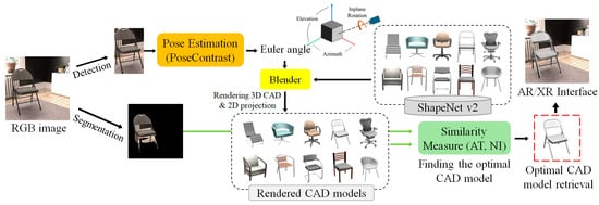
Figure 1.
The architecture of the proposed 6-DoF pose estimation and CAD retrieval method.
In the experiment, we show that the enhanced pose estimation performance also enhances the performance of CAD model retrieval. The performance relationship between the pose estimation and CAD model retrieval is quantitatively analyzed by a correlation parameter. The structure of this paper is as follows. In Section 2, we briefly explain camera parameters related to this study. Section 3 describes all the steps of the proposed method. In Section 4, we show several quantitative and qualitative evaluation results. Section 5 presents the ablation study for the proposed pose estimation model. Finally, in Section 6, we conclude this paper.
2. Internal and External Pose Parameters
The 6-DoF pose estimation of a 3D object in an RGB camera image is to determine the external orientation and translation of the object from a reference coordinate system to the camera coordinate system. In addition, the projection of the transformed 3D object into the image plane is expressed by the internal camera parameters. If we know the 6-DoF pose of the object and the camera parameters, we can transform and project a shape-matching CAD model into the image space so that the projection exactly aligns with the object area.
To project a 3D CAD model into an RGB image space, it is essential to understand the projection of a 3D point into the image plane. Let be a point in the 3D space (reference coordinate system), the corresponding point in the camera coordinate system, and the projected point in the image plane (pixel coordinate system). Point is determined through the following Equations (1)–(3). We assume where represents the focal length of the camera.
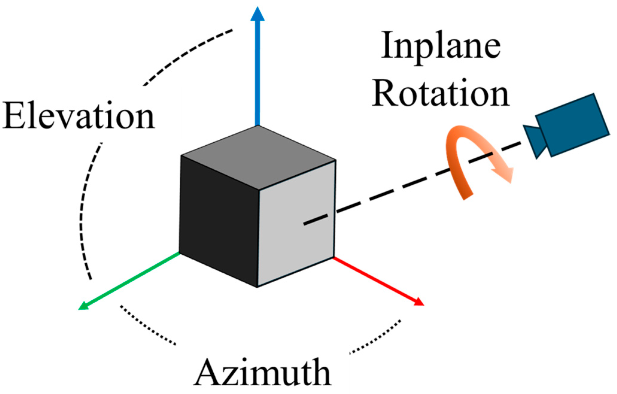
In this paper, the 3-DoF rotation parameters are represented by the Euler angles, as shown in Figure 2. The other 3-DoF is related to the translation between the reference to the camera coordinate systems. Among the 3-DoF translation parameters, the translation along the z-axis affects the size of the object in the image plane, as the size is affected by both the translation along the z-axis and the camera’s focal length (). The camera translations along the x and y axes, and , do not affect the object’s size. However, estimation of z-axis translation has inherent ambiguity because the object size is also affected by the focal length. Therefore, to estimate the 3-DoF parameters associated with the translation, both and the two scale factors () should be estimated.

Figure 2.
Representation of 3-DoF rotation from the reference to the camera coordinate systems.
3. Proposed Methods
3.1. Dataset for Reference CAD Models
Pascal3D+ [22] has been commonly used in many 6-DoF pose estimation studies. This study also uses Pascal3D+ to train the proposed pose estimation network. In addition, we use Pascal3D+, Pix3D [23], and ObjectNet3D [24] as the test datasets. The Pascal3D+ dataset consists of 12 categories, including airplanes, bicycles, chairs, and automobiles, and consists of approximately 36,000 images. Among these, 28,100 images are used for training, and 2113 images are used for testing. The Pix3D dataset contains 9 indoor object categories, generally categorized for IKEA household items, with about 10,000 images. Among them, the chair category contains the largest portion, with around 4000 images. ObjectNet3D includes 100 categories and consists of approximately 90,000 images. Unlike the previous two datasets, ObjectNet3D encompasses categories for relatively small objects such as keys, pencils, and pens.
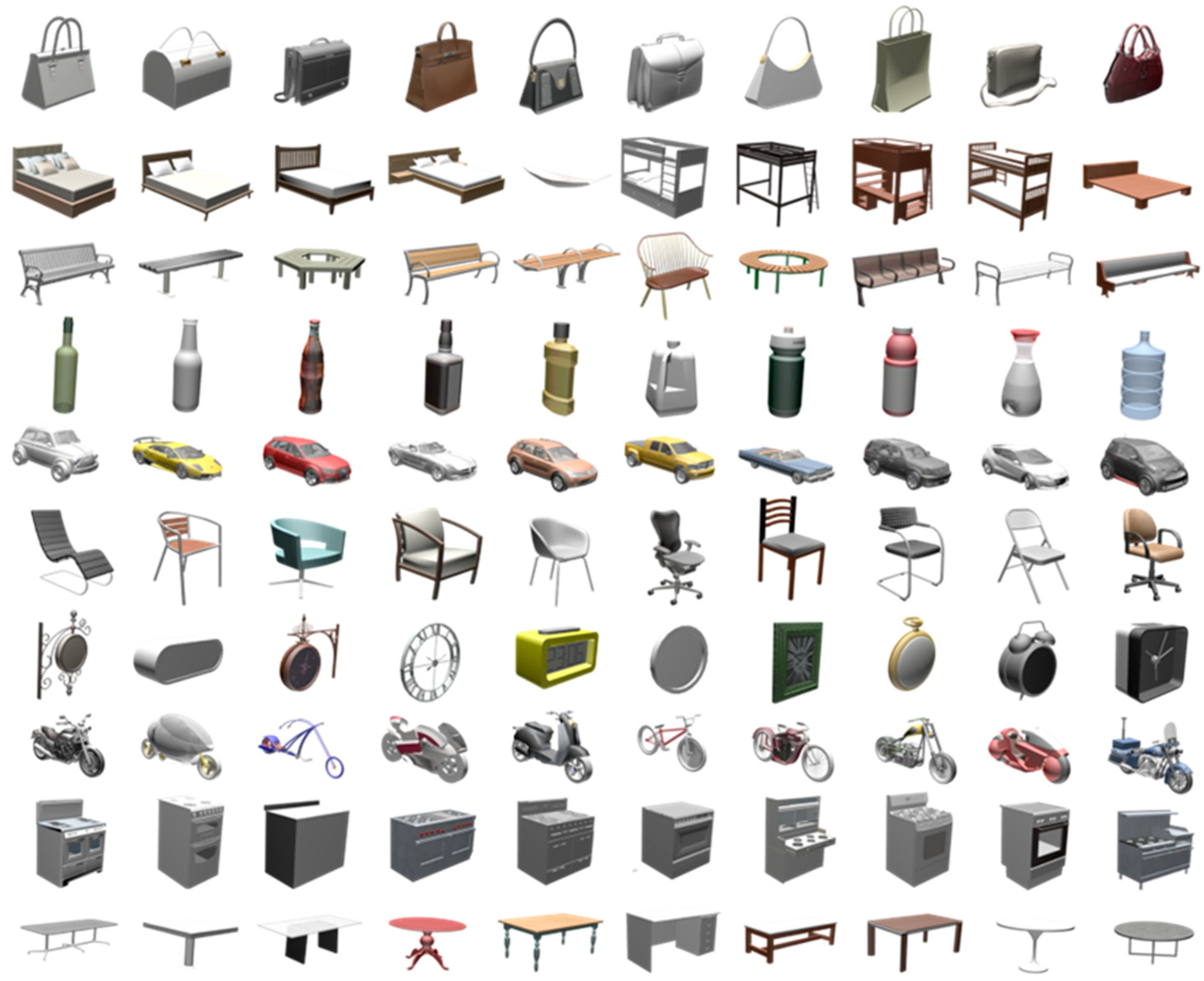
For CAD model retrieval, the 3D CAD dataset from ShapeNetCore is used. It is a subset of the ShapeNet [12] database. ShapeNetCore provides 3D CAD models across 55 upper categories for indoor and outdoor objects, with various subcategories. In this study, 10 upper categories (bag, bed, bottle, bench, car, chair, clock, motorcycle, stove, and table) and 10 subcategories within each category are selected, resulting in a total of 100 CAD models. The selection criteria for these categories are based on the following principles, and the 100 CAD models are shown in Figure 3.

Figure 3.
For CAD model retrieval, 10 CAD object categories with 10 subcategories are used.
- The upper category should have a matching category in the Microsoft COCO dataset [25] because the object detection network is trained on this dataset.
- The appearance of the CAD models in a subcategory should be different enough to facilitate similarity measurement.
- The appearance and shape of the CAD models across all categories should be general so that they appear in a sufficient amount of RGB image data.
3.2. Dataset for RGB Images
The RGB images were collected by the authors from Google Images and Bing Search Images, along with the 100 reference CAD models. The criteria for the collection of RGB images are summarized below. A total of 20 RGB images were collected for each model, resulting in a total of 2000 RGB images.
- To ensure usability in object detection and pose estimation networks, the image size is constrained between 224 × 224 and 1600 × 1600 pixels.
- Accepted image formats include jpg, jpeg, and png.
- For similarity measurement between the RGB object and the CAD rendering, it is necessary that the RGB object is minimally occluded.
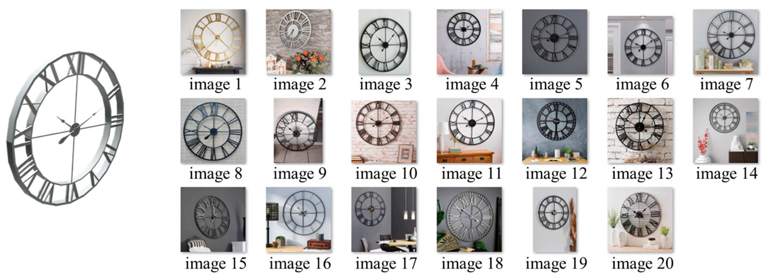
Given a single RGB image, object detection and segmentation are performed using DetectoRS [20]. If there is no detected object in the image, it is excluded from the dataset. Furthermore, when multiple types of objects are detected within a single RGB image, it is used when any object in the image is in the same category as one in the CAD dataset. When the objects in an image are different types from the CAD dataset, it is excluded. For images with multiple instances of the same object, all instances are retained. Following this inclusion and exclusion process, a total of 1562 RGB images are used for CAD model retrieval. Figure 4 shows examples of RGB images collected for a clock CAD model.

Figure 4.
Example of 20 RGB images collected for a clock CAD model.
3.3. Proposed Pose Estimation Network
As mentioned in an earlier section, the proposed 6-DOF pose estimation is performed by a deep learning network whose baseline is PoseContrast [17]. PoseContrast estimates the rotational pose of an object from a single RGB image. This network uses ResNet50 [26] as the encoder backbone and a multilayer perceptron (MLP) as the predictor. Here, the 3-DoF rotational pose is represented by three Euler angles from the reference CAD coordinate system to the camera coordinate system. The three Euler angles are defined as Azimuth, Elevation, and Inplane rotation. In PoseContrast, each rotation angle is predicted into 15° sized bins with an offset value ranging from −1 to +1. The final rotation angle is then calculated as in Equation (4).
The loss functions employed in the bin prediction and offset prediction are Cross Entropy Loss [27] (Equation (5)) and Smooth L1 Loss [28] (Equation (6)), respectively. In Equation (5), and can be considered as bin vectors of MLP prediction and GT, respectively. Each bin vector consists of 24 elements of probability to each 15° bin. In Equation (6), is the MLP prediction to the angle offset. In PoseContrast, the same loss functions are applied to predict all three rotation angles.
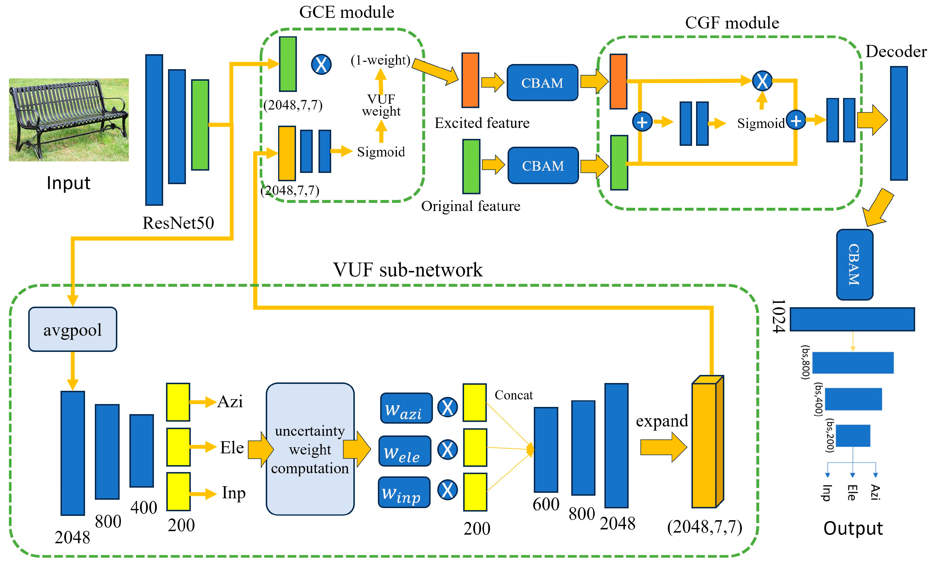
In this paper, we modify the original PoseContrast network by adding one sub-network (VUF) and two attention modules (GCE and CGF) to the original network. The structure of the proposed network is illustrated in Figure 5. First, we introduce a sub-network that generates variational uncertainty features from the output of ResNet50. The sub-network generates uncertainty features and they are used to generate the uncertainty weight to the original ResNet50 features. Thus, we call this sub-network the VUF (Variational Uncertainty Feature) network.

Figure 5.
Architecture of our proposed pose estimation network.
Similar to the original PoseContrast, VUF also predicts Azimuth, Elevation, and Inplane rotation using two MLP networks, as shown in Figure 5. The first MLP provides the probability to each angle bin, and the highest bin index is determined based on the probability values. The output of the first MLP is used to compute the uncertainty weight of each angle bin, as shown in the figure. To compute the uncertainty weight, is first calculated as in Equation (7) to represent the degree of difference between the highest probability bin index , and another bin index . To provide smooth weight values to the next process, the bin angle difference is represented in the logarithm scale as in Equation (7). Once in each angle bin is obtained, , variance uncertainty, is calculated using Equation (8). Here, is the probability of bin index i. The final weight, , for each angle bin is calculated as in Equation (9). This process is applied respectively to Azimuth, Elevation, and Inplane rotation.
where, .
where, .
Weight obtained in Equation (9) is multiplied to the original features trained for angle prediction. In each angle prediction, the features consist of 200 channels. The weighted 200 features are then concatenated to form an integrated feature module. Through the second MLP, the integrated feature module is then refined and expanded to a feature map of size 2048 × 7 × 7, which is the same size as the original feature map from the ResNet50.
Our second modification consists of two modules, the Guided Cost Volume Excitation (GCE [29]) module and the Context and Geometry Fusion (CGF [30]) module, as shown in Figure 5. The main purpose of adding two modules is to fuse the feature map from the original ResNet50 and the features from the VUF sub-network. Through the two modules, the features from ResNet50 are excited to predict the angular pose of an object. Following the GCE module, a Convolutional Block Attention Module (CBAM [31]) is applied to extract key features from the excited features and the original features. CBAM provides more attention to the key features; consequently, it enhances the pose estimation performance. These features are then processed through the CGF module, which generates a spatial attention weight. Finally, CBAM is applied again to the feature, and then it is used as input for the predictor.
In addition to the new sub-network and module employment, we enhance the proposed network by introducing a new loss function. Conventionally, the cross entropy loss function in Equation (5) computes the uniform loss between the prediction and the ground truth. For instance, when predicting an Azimuth angle with a GT angle of 0°, the prediction of 15° differs significantly from 225° in terms of angle difference. However, the cross entropy calculates both losses as the same magnitude. To address this issue, we propose a quaternion-based loss function. Quaternion is a generalized form of a complex number comprising three real components and one imaginary component, as shown in Equation (10). To employ the quaternion-based loss function, we convert the rotation angles from PoseContrast and the ground truth (GT) into quaternions using Equations (11)–(14). Here, Azimuth is denoted as , Elevation as and Inplane rotation as . Equation (15) shows the quaternion loss function, with the parameter α empirically set to 3. Given the importance of accurately predicting the bin index, we formulate the final loss function by integrating the quaternion loss into the existing loss function.
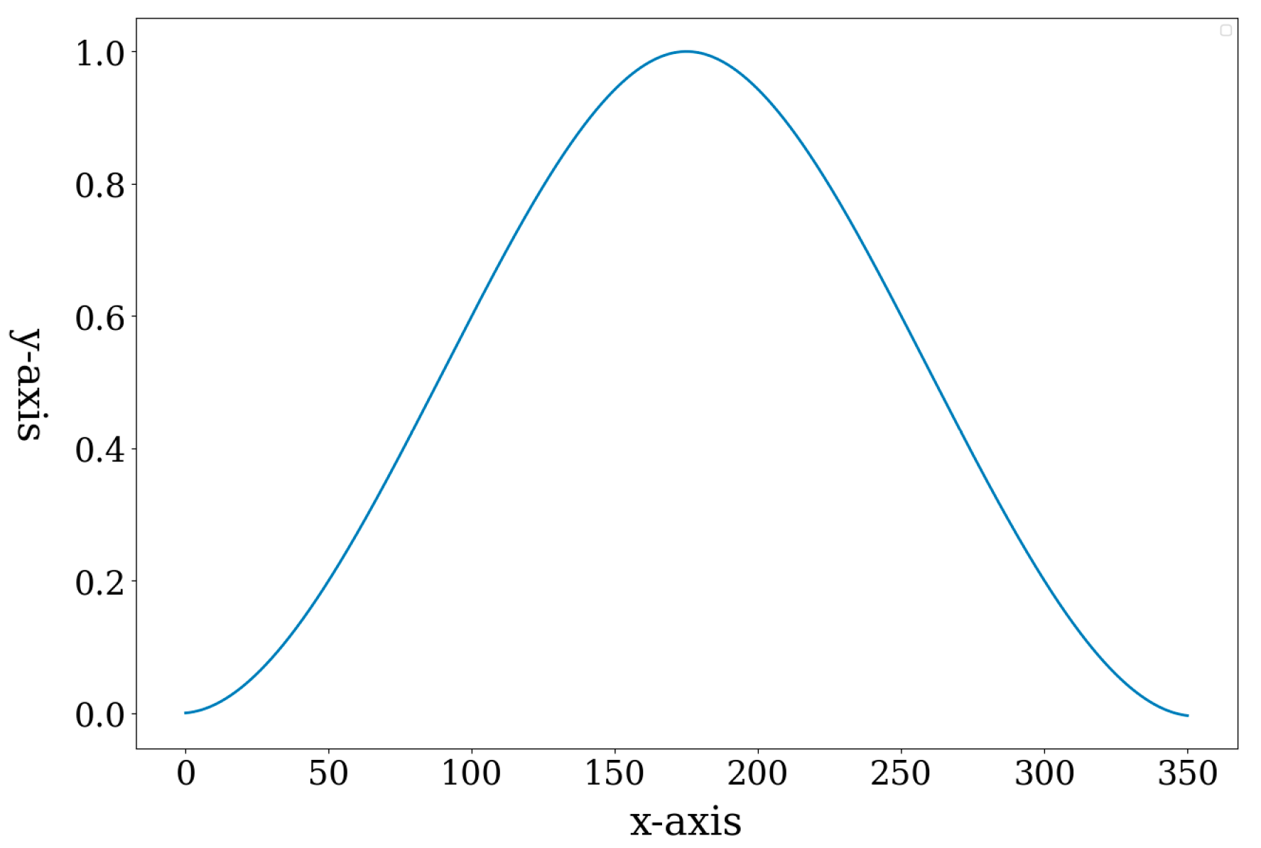
The quaternion-based loss function solves the issue of uniform loss between predicted and GT bin indices in the cross entropy loss function. For example, when the GT bin index is 0 and the predicted bin index is 1 (15°) or 15 (225°), the network is trained with different loss values. On the contrary, when the predicted bin is 23 (335°) or 1 (15°), the same loss value is obtained because they are equidistant from the GT. Especially, when the predicted bin index is 12, exactly opposite angle to the GT bin, the loss value becomes maximum, as shown in Figure 6. By employing these non-uniform loss values, the proposed quaternion-based loss function enhances the performance of angular pose estimation with the proposed network.

Figure 6.
An example of quaternion-based loss function (α = 1, GT index = 0). The X-axis represents the bin index, and the y-axis represents loss value.
3.4. Similarity Measurement Between RGB Image and CAD Rendering
Using the modified PoseContrast network, the rotational pose of a real object in a single RGB image has been predicted. Using the predicted rotational pose, we can transform a CAD model from the reference to the camera coordinate system. However, to apply the proposed 6-DoF pose estimation technique to AR or XR applications, it is necessary to retrieve and transform the CAD model whose category and shape match exactly with the RGB object. However, because the PoseContrast network is a class-agnostic pose estimator, we need to find the exact subcategory of the RGB object before projecting the CAD model to the image space.
Until the previous section, we have known that the upper category of an RGB object from the DetectRS network. However, there are various shapes of CAD models in the same upper category from the dataset. Examples of the bench category in the ShapeNetCore are shown in Figure 7. On the left side of the figure is a bench RGB image and the right side shows bench CAD models. On the right side, 10 different shapes of the bench category are shown, and in this study, we call each different shape a subcategory.

Figure 7.
Rendering of 10 CAD subcategories using the pose estimation result of a bench object.
This section describes how to determine the best matching subcategory from 10 candidate models. To find a matching subcategory, we employ a deep feature matching network, DELF (Large-Scale Image Retrieval with Attentive Deep Local Features) [19]. As shown in Figure 7, the rotational pose estimation result is used to transform candidate CAD models to the camera coordinate system and to render them into the 2D image plane. Therefore, using DELF, we propose to measure 2D image similarity between the RGB object and the rendered CAD images and to determine the best similar rendering as the final matching model.
Details of similarity measurement are as follows. First, the background of the RGB object is removed using the DetectRS segmentation result. Second, we obtain 10 rendered images of subcategories. Third, between each pair of the RGB object and rendered image, we derive a 2D affine transformation matrix using DELF. From the DELF feature detection and RANSAC outlier removal, we obtain the affine transformation matrix. The motivation for obtaining a 2D affine matrix is that the ideal image space transformation between the RGB object and the rendered CAD model is only unknown scaling. The ideal rotational pose of the matching CAD model results in only scale difference with unknown z-axis translation and focal length.
The 2D affine transformation matrix in Equation (16) consists of six elements representing 2D rotation, scaling, and skewing transformations, as well as translation. In this equation, two translation elements are not needed because only rotational pose is applied to the CAD rendering. Thus, only the front 2 × 2 matrix in is considered, and it is defined as matrix , as in Equation (17). The four elements of consist of multiplications of scale (S), skew (,) and 2D rotation ().
The first image similarity measurement is based on the 2D affine transformation, called SM-AT. The size of the 2D rendering image is fixed at 600 × 600 pixels, whereas the size of RGB object images varies significantly in the collected dataset. Therefore, even if the rotational poses of the RGB object and CAD rendering are identical, there is still an image scale difference. Thus, practically, the 2D rotation transformation between RGB and CAD rendering should not be an identity matrix but rather multiplied by two scale factors, as shown in Equation (18). As the rotational pose between the RGB object and the CAD rendering becomes similar, matrix should have only scale elements in Equation (18). In the ideal case, if the rotational poses in both RGB and CAD rendering images are the same, and . Here, scale S can be obtained from Equation (19). To normalize , we derive the scale-normalized affine matrix as in Equation (20).
From the scale-normalized matrix , we define and using Equations (22) and (23). Finally, the rank for CAD model retrieval is determined by the value as in Equation (24), where a higher value means a higher rank. Additionally, by defining as in Equation (24), we consider not only the error for the rotation angle but also the affine consistency for retrieving the matching CAD model. In Equation (24), is the number inlier in deriving the affine transformation matrix .
As the second measurement, we only use the number of feature-matching inliers (SM-NI). With this measurement, the CAD retrieval ranking is determined from the highest number of inliers to the lowest number.
Using these two measurements, the similarity between every pair of RGB image and CAD rendering image within a detected upper category is evaluated. For the evaluation of the two measurements, we have manually generated the annotations of CAD subcategories for all 2000 RGB images. In the experiments, we show quantitative analysis of CAD model retrieval based on SM-AT and SM-NI with the ground truth.
3.5. Translation and Focal Length Estimation
After retrieving the matching CAD model, it is now possible to estimate the scale factor ( by projecting the CAD model to the RGB image space. In the pin-hole camera model, the projection size of the CAD model is affected by both and . However, solving both parameters together is an ambiguous problem. Thus, one parameter must be set as an arbitrary value while the remaining parameter is estimated. In this study, we define the limited range of focal length and z-axis translation because there is no GT focal length parameter in the RGB images from the Internet. Using the limited ranges and an iterative algorithm, we estimate both parameters.
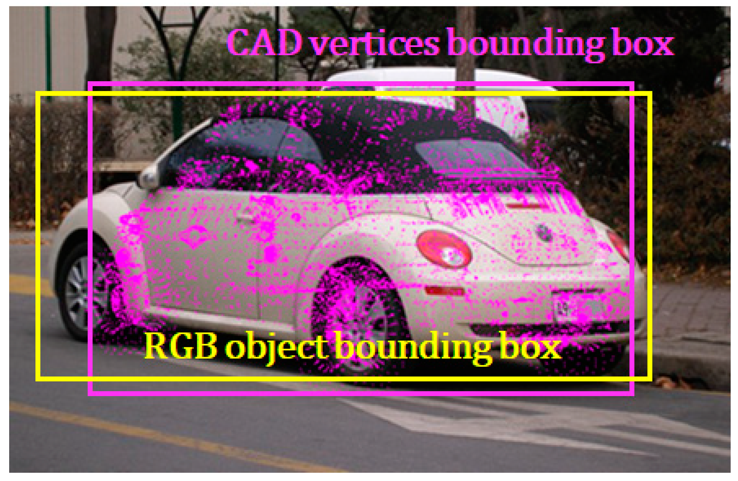
In this iterative algorithm, and are set to 0 because we assume the center of the bounding box corresponds to the center of the object. By the pin-hole camera model, a 3D vertex point on the 3D CAD model is projected to a 2D image point , where and is the number of vertices in the 3D CAD model. The scale parameters are ranged as follows: and . Principal points and are decided to be at the center of the cropped image. By applying these values from Equations (1)–(3), the 3D vertices are projected into the image plane. A new bounding box is created using the 2D projection points such as and . Then, the Intersection Over Union (IoU) between this newly created bounding box and the existing RGB object bounding box is calculated. The values of and that maximize the IoU are selected as the final estimation. An example of CAD vertex projection and bounding boxes is shown in Figure 8.

Figure 8.
Projection result of a car CAD model.
After estimating the scale factor, and must be recalculated from the original RGB image using Equations (1)–(3). Principal points and represent the center points of the original image. Scale factors are estimated from the cropped image without changing the pixel size; thus, these values remain valid in the original image. Since the center of the 3D CAD model is at the origin of the reference coordinate system, and can be determined by Equations (1)–(3). By setting and projecting it to the image space, we have the center of the 2D bounding box in the cropped RGB images. In the original image space, the center of the projected bounding box becomes , where is the upper-left corner of the bounding box in the original image. Then external translation and can be calculated as:
4. Experiment and Evaluation
4.1. Experimental Setup
We trained the proposed pose estimation network using Adam optimizer with a batch size of 16 and an initial learning rate of . We trained for 15 epochs on an Intel Xeon CPU with a single NVIDIA A5000 GPU equipped with 24 GB memory (Santa Clara, CA, USA).
4.2. Evaluation of Pose Estimation
We evaluated the pose estimation performance through two quantitative metrics, Acc30 and Median Error, as described in [32,33]. Acc30 evaluates the proportion of instances where the angular difference between the predicted and GT angles is within 30°. It is measured in percentage (%). Equations (26)–(31) show the conversion process of Euler angles into rotation transformation matrices, where and denote Azimuth, Elevation, and Inplane rotation, respectively. Median Error quantifies the median of the differences in rotational angles between the predicted and ground truth values, measured in degrees (°).
The performance was compared with PoseContrast using three test datasets, Pix3D, Pascal3D+, and ObjectNet3D, as shown in Table 1, Table 2 and Table 3. We trained our proposed model using the Pascal3D+ dataset. We tested the model on the Pix3D and ObjectNet3D datasets to evaluate generalization performance. Table 1 presents the quantitative results on Pascal3D+, showing that the proposed method outperforms the baseline, PoseContrast. Moreover, as shown in Table 2 and Table 3, our model performs better than the PoseContrast in generalization evaluations.

Table 1.
Pose estimation performance using Pascal3D+ (number of images is in parenthesis and bold font indicates the best performance in each column).

Table 2.
Pose estimation performance using Pix3D (number of images is in parenthesis and bold font indicates the best performance in each column).

Table 3.
Pose estimation performance using ObjectNet3D.
Employing two evaluation metrics enables complementary analysis. Evaluation only using Acc30 might lead to misleading conclusions; for instance, an error of 31° would be classified as incorrect despite being very close to the reference angle. Consequently, incorporating Median Error provides the distribution of errors, which is a more comprehensive evaluation for performance comparison.
4.3. Evaluation of CAD Model Retrieval
Table 4 presents the evaluation results of CAD model retrieval using 1562 RGB images. Originally, 2000 RGB images were used for CAD model retrieval; however, 438 images were rejected from the test by the rules described in Section 3.2. The matching CAD model with the RGB object is retrieved based on the image similarity between the RGB object and the CAD rendering images. Given an RGB object, renderings of the 10 subcategories of CAD models are ranked from 1st to 10th. In Table 4, the number of RGB images that find the matching CAD models among the top five rankings is shown.

Table 4.
Number of RGB images that retrieve the matching CAD model as the specific rank.
For the SM-AT method, the rate of retrieving the matching CAD model within the top three rankings is 72.087%, and within the top five rankings, it is 85.147%. For the SM-NI method, these rates are 75.416% and 87.708%, respectively. These results show that both similarity measurements are useful for evaluating the similarity between the RGB image and the CAD image domains.
4.4. Correlation Analysis Between Pose Estimation and CAD Retrieval
This study addresses not only the 6-DoF pose estimation of RGB objects but also CAD model retrieval for the purpose of AR and XR applications. Thus, it is expected that the performance enhancement of the proposed pose estimation positively affects the performance of the CAD retrieval. In this section, we investigate qualitative and quantitative analysis to verify the positive relationship between the performance of the two tasks.
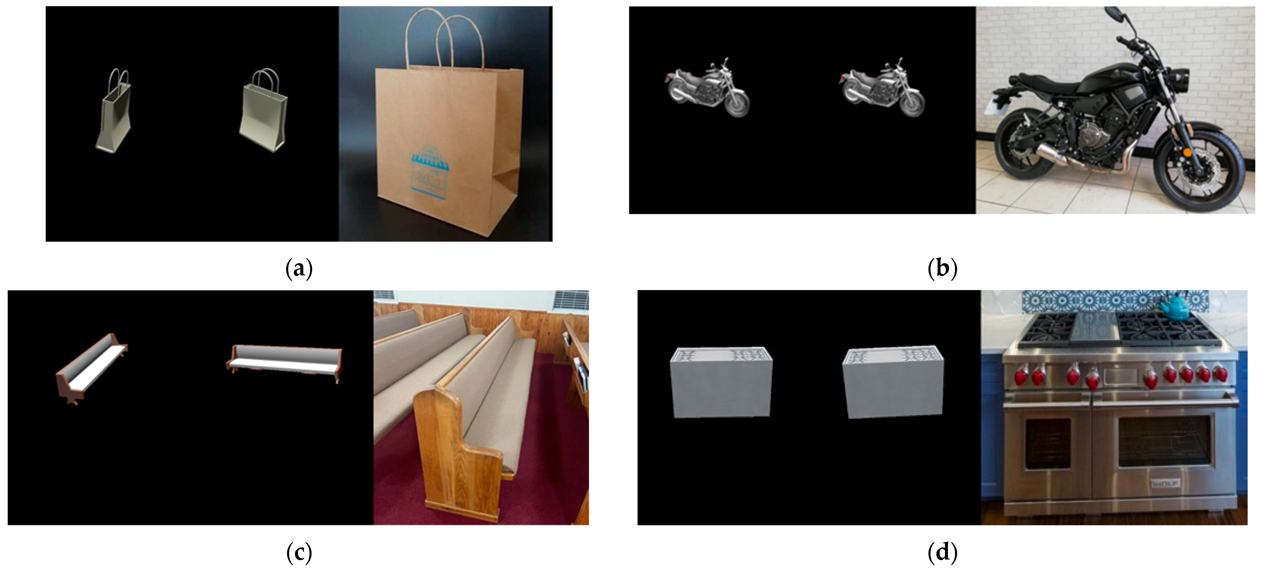
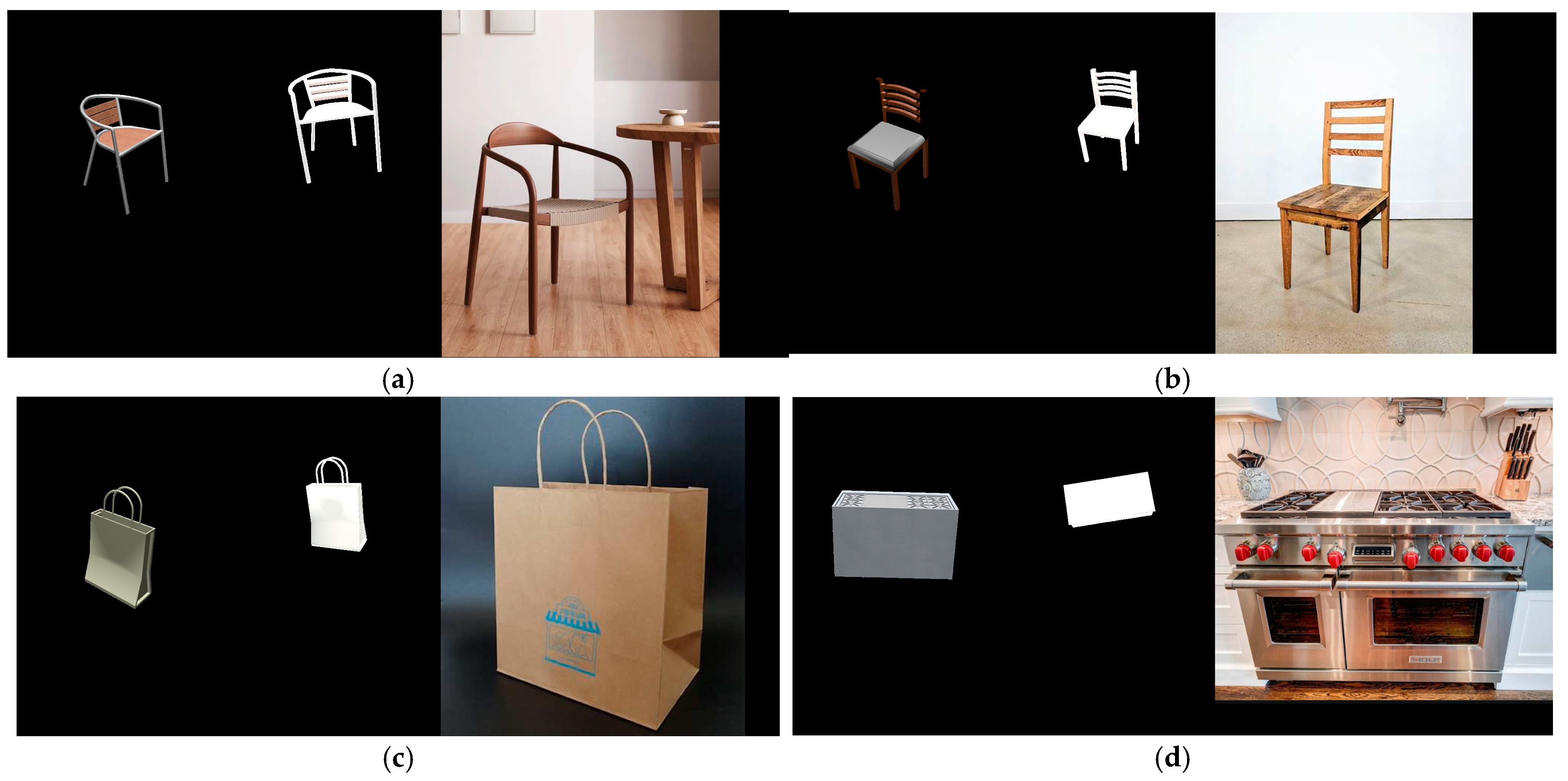
First, we evaluate the performance relationship qualitatively. In this evaluation, we visually compare 2D rendered images of the matching CAD model with the RGB object. If the predicted pose perfectly matches with the RGB object, then the pose appearance should be very similar. The visual comparison is performed with two conventional methods: one is PoseContrast, and the other is PosefromShape. In each comparison, we generate a side-by-side rendering image pair from the conventional and the proposed methods, as shown in Figure 9. For each RGB test image, the side-by-side rendering image pair is concatenated, and their poses are visually compared. Based on the comparison, we classify the results into four cases:

Figure 9.
Samples of CAD renderings and RGB images. From the left, renderings from PoseContrast, the proposed method, and the RGB object. The qualitative comparison is (a) Better, (b) SS, (c) Worse, and (d) Bad.
- Better: Rendering images from the proposed network yields a better pose appearance than the conventional method. An example is shown in Figure 9a and Figure 10a.
 Figure 10. Samples of CAD renderings and RGB images. From the left, renderings from the proposed method, PosefromShape, and RGB object. The qualitative comparison is (a) Better, (b) SS, (c) Worse, and (d) Bad.
We consider that the predicted rotational pose is significantly different from the RGB object if the pose difference is more than about 45°. For the performance correlation analysis, the ‘Bad’ case is excluded. In Figure 9, the left image is the estimation result from PoseContrast, the center image is from the proposed method, and the right image is RGB objects.
Table 5 and Table 6 present the results of the qualitative evaluation. Each evaluation is denoted as ‘Better’, ‘SS’, and ‘Worse’, respectively. Table 5 shows the evaluation with respect to PoseContast and Table 6 is to PosefromShape. The greater number of ‘Better’ evaluations is obtained in Table 6 because the performance enhancement compared to PosefromShape is much higher than that of PoseContrast. For comparative analysis with PosefromShape, we evaluate this method using the same dataset as our proposed method. Unlike PoseContrast, which predicts the pose from a single RGB image and renders the CAD model using the same predicted angle for all instances, PosefromShape predicts individual values for each pair of an RGB image and a CAD model used as input. Therefore, for our evaluation, we use the rendering of the ground truth CAD model to estimate the similarity measurement.

Table 5.
Results of the qualitative evaluation compared to PoseContrast (number of detected images is in parenthesis).

Table 6.
Results of the qualitative evaluation compared to PosefromShape (number of detected images is in parenthesis).
Using the visual evaluation of the pose estimation, we performed an additional quantitative analysis by introducing a correlation score between the pose estimation and the CAD retrieval. In Table 4, we have shown the rank numbers of the matching CAD model using the two image similarity measurements.
Let be the rank number of the matching CAD model with the i-th test RGB images, the rank number results from the proposed method, and the rank number results from the conventional methods, PoseContrast or PosefromShape. We use Equation (32) to get the correlation score of the i-th test image. This simple equation gives a positive reward score if the image similarity rank from the proposed method is higher (rank number becomes small) than that from PoseContrast or PosefromShape. On the contrary, this equation gives a negative score if the image similarity rank from the proposed method is lower (rank number becomes large).
For example, if the matching CAD model is ranked 1st using the proposed network and 3rd using a conventional method, the score is +2. On the contrary, if the conventional method yields a better rank, we give a negative score. If both results yield the same rank, the score is 0. The proposed correlation score is based on the rank difference between the two networks rather than the absolute rank obtained from each network. After adding all scores from all RGB images, we get the average by dividing by the number of all RGB images. Table 7 and Table 8 show the correlation score of the proposed method with two image similarity measurements. In both measurements, a positive score is obtained in the ’Better’ case, while a negative score is obtained in the ’Worse’ case. Additionally, the ’SS’ case yields a score close to zero. This quantitative analysis shows that the performance improvement from the proposed pose estimation method also improves the performance of CAD model retrieval. In addition, the pose estimation failures also negatively affect the CAD model retrieval. As shown in Table 8, correlation scores with respect to PosefromShape, the positive correlation scores in the ‘Better’ case are higher than those in Table 7. This means that the correlation score evaluation with respect to PosefromShape is much higher than PoseContrast.

Table 7.
Correlation score per sample between pose performance and similarity measurement. Pose performance comparison is with respect to PoseContrast.

Table 8.
Correlation score per sample between pose performance and similarity measurement. Pose performance comparison is with respect to PosefromShape.
5. Ablation Study of the Proposed Pose Estimation Model
In this section, we perform ablation experiments on the Pascal3D dataset to validate the effectiveness of the proposed model. Unlike the baseline model, the proposed model includes three key modules and is trained using an additional quaternion loss function. Table 9 shows how we have conducted ablation studies for each of these modules. All model variants were trained under the same conditions outlined in the implementation details. Table 10 presents the results for each modified model. In Table 9, VUF refers to the variance uncertainty model in our proposed approach, GCE denotes the Guided Cost Volume Excitation module, CGF refers to Context and Geometry Fusion, and Q loss specifies whether a quaternion loss was employed during training.

Table 9.
Configurations of the ablation models. The baseline model is PoseContrast.

Table 10.
Comparison of the quantitative results of the ablation models. The baseline model is PoseContrast. The best performance is highlighted in bold.
As shown in Table 10, adding the proposed modules to the baseline progressively improves performance. Specifically, the VUF module alone shows little improvement over the baseline. The VUF module leverages variance uncertainty for each predicted angle to enhance performance; however, it incurs feature loss during the module’s internal attention process, so an additional auxiliary module is required to boost performance further. By supplementing VUF with the GCE module (VUF+GCE), the network compensates for this loss and improves performance, as observed in Table 10. Next, to assess the effect of the quaternion loss function, we compare the proposed model to a VUF-full ablation variant that excludes the quaternion loss. The results show that the addition of the quaternion loss during training enhances the performance of the proposed method.
6. Conclusions
In this study, we propose 6-DoF pose estimation and CAD model retrieval methods to align the projection of the CAD model with an object in an RGB image. The pose estimation is performed by using a deep learning network which is based on the PoseContrast network. To enhance the performance of the class-agnostic PoseContrast network, we add two sub-networks to emphasize the feature weight from the original ResNet50. Variance uncertainty weight and attention sub-network modules enhance the performance of pose estimation. After the pose estimation of the RGB object, we retrieve the matching CAD model from a CAD dataset. The quantitative analysis of the correlation between the 6-DoF pose estimation and the CAD model retrieval has been conducted. We evaluate the performance of pose estimation on Pascal3D+, Pix3D, and ObjectNet3D datasets. Through the experiments, we show that the proposed network reduces median errors in calculating the rotation angle of a 3D object in the RGB image. Furthermore, it is shown that the matching CAD model can be effectively retrieved using two similarity measurements (SM-AT and SM-NI). In addition, we find that there is a positive correlation between the pose estimation and CAD model retrieval performances.
In our experiments, there is a limitation in the training stage of the proposed network. The Pascal3D+ dataset, used for training, exhibits a bias in the distribution of Euler angles of the RGB objects. This bias may affect the network’s ability to estimate the pose of the objects. In future studies, we will focus on developing a new training dataset with evenly distributed training angles.
Author Contributions
Conceptualization, S.-Y.P.; methodology, software, validation, formal analysis, S.P., M.M. and W.-J.J.; investigation, S.P., W.-J.J., M.M. and S.-Y.P.; writing—original draft preparation, S.P. and W.-J.J.; writing—review and editing, S.-Y.P.; supervision, S.-Y.P.; project administration, S.-Y.P.; funding acquisition, S.-Y.P. All authors have read and agreed to the published version of the manuscript.
Funding
This research was supported partly by Institute of Information & Communications Technology Planning & Evaluation (IITP) grant funded by the Korea government (MSIT) (No.2021-0-00320, Manipulation and Augmentation for XR in the Real-World Environment) and partly by Culture, Sports and Tourism R&D Program through the Korea Creative Content Agency grant funded by the Ministry of Culture, Sports and Tourism in 2024 (No. RS-2024-00341886).
Institutional Review Board Statement
Not applicable.
Informed Consent Statement
Not applicable.
Data Availability Statement
The raw data supporting the conclusions of this article will be made available by the authors on request.
Conflicts of Interest
The authors declare no conflicts of interest.
References
- Wang, S.; Clark, R.; Wen, H.; Trigoni, N. DeepVO: Towards End-to-End Visual Odometry with Deep Recurrent Convolutional Neural Networks. In Proceedings of the 2017 IEEE International Conference on Robotics and Automation (ICRA), Singapore, 29 May–3 June 2017; pp. 2043–2050. [Google Scholar]
- Lowe, D.G. Distinctive Image Features from Scale-Invariant Keypoints. Int. J. Comput. Vis. 2004, 60, 91–110. [Google Scholar] [CrossRef]
- Bay, H.; Ess, A.; Tuytelaars, T.; Van Gool, L. “Speeded-Up Robust Features (SURF). ” Comput. Vis. Image Underst. 2008, 110, 346–359. [Google Scholar] [CrossRef]
- Rublee, E.; Rabaud, V.; Konolige, K.; Bradski, G. ORB: An Efficient Alternative to SIFT or SURF. In Proceedings of the 2011 International Conference on Computer Vision, Barcelona, Spain, 6–13 November 2011; IEEE: New York, NY, USA; pp. 2564–2571. [Google Scholar]
- Besl, P.J.; McKay, N.D. A Method for Registration of 3-D Shapes. IEEE Trans. Pattern Anal. Mach. Intell. 1992, 14, 239–256. [Google Scholar] [CrossRef]
- Fischler, M.A.; Bolles, R.C. Random Sample Consensus. Commun. ACM 1981, 24, 381–395. [Google Scholar] [CrossRef]
- Xiang, Y.; Schmidt, T.; Narayanan, V.; Fox, D. PoseCNN: A Convolutional Neural Network for 6D Object Pose Estimation in Cluttered Scenes. arXiv 2018, arXiv:1711.00199. [Google Scholar]
- Do, T.-T.; Cai, M.; Pham, T.; Reid, I. Deep-6DPose: Recovering 6D Object Pose from a Single RGB Image. arXiv 2018, arXiv:1802.10367. [Google Scholar]
- Kendall, A.; Grimes, M.; Cipolla, R. PoseNet: A Convolutional Network for Real-Time 6-DOF Camera Relocalization. In Proceedings of the 2015 IEEE International Conference on Computer Vision (ICCV) IEEE, Santiago, Chile, 7–13 December 2015; pp. 2938–2946. [Google Scholar]
- Dong, Z.; Liu, S.; Zhou, T.; Cheng, H.; Zeng, L.; Yu, X.; Liu, H. PPR-Net:Point-Wise Pose Regression Network for Instance Segmentation and 6D Pose Estimation in Bin-Picking Scenarios. In Proceedings of the 2019 IEEE/RSJ International Conference on Intelligent Robots and Systems (IROS), Macau, China, 3–8 November 2019; IEEE: New York, NY, USA; pp. 1773–1780. [Google Scholar]
- Wang, C.; Xu, D.; Zhu, Y.; Martin-Martin, R.; Lu, C.; Fei-Fei, L.; Savarese, S. DenseFusion: 6D Object Pose Estimation by Iterative Dense Fusion. In Proceedings of the 2019 IEEE/CVF Conference on Computer Vision and Pattern Recognition (CVPR), Long Beach, CA, USA, 16–20 June 2019; IEEE: New York, NY, USA; pp. 3338–3347. [Google Scholar]
- Zakharov, S.; Shugurov, I.; Ilic, S. DPOD: 6D Pose Object Detector and Refiner. In Proceedings of the 2019 IEEE/CVF International Conference on Computer Vision (ICCV), Seoul, Republic of Korea, 27 October–2 November 2019; IEEE: New York, NY, USA; pp. 1941–1950. [Google Scholar]
- Xu, Y.; Lin, K.-Y.; Zhang, G.; Wang, X.; Li, H. RNNPose: Recurrent 6-DoF Object Pose Refinement with Robust Correspondence Field Estimation and Pose Optimization. In Proceedings of the 2022 IEEE/CVF Conference on Computer Vision and Pattern Recognition (CVPR), New Orleans, LA, USA, 21–24 June 2022; IEEE: New York, NY, USA; pp. 14860–14870. [Google Scholar]
- Hu, N.; Zhou, H.; Liu, A.-A.; Huang, X.; Zhang, S.; Jin, G.; Guo, J.; Li, X. Collaborative Distribution Alignment for 2D image-based 3D shape retrieval. J. Vis. Commun. Image Represent. 2022, 83, 103426. [Google Scholar] [CrossRef]
- Park, S.-Y.; Son, C.-M.; Jeong, W.-J.; Park, S. Relative Pose Estimation between Image Object and ShapeNet CAD Model for Automatic 4-DoF Annotation. Appl. Sci. 2023, 13, 693. [Google Scholar] [CrossRef]
- Gümeli, C.; Dai, A.; Nießner, M. ROCA: Robust CAD Model Retrieval and Alignment from a Single Image. In Proceedings of the 2022 IEEE/CVF Conference on Computer Vision and Pattern Recognition (CVPR), New Orleans, LA, USA, 19–24 June 2022; pp. 4012–4021. [Google Scholar]
- Xiao, Y.; Du, Y.; Marlet, R. PoseContrast: Class-Agnostic Object Viewpoint Estimation in the Wild with Pose-Aware Contrastive Learning. In Proceedings of the 2021 International Conference on 3D Vision (3DV), London, UK, 1–3 December 2021; IEEE: New York, NY, USA; pp. 74–84. [Google Scholar]
- Tang, J.; Chen, Z.; Fu, B.; Lu, W.; Li, S.; Li, X.; Ji, X. ROV6D: 6D Pose Estimation Benchmark Dataset for Underwater Remotely Operated Vehicles. IEEE Robot. Autom. Lett. 2024, 9, 65–72. [Google Scholar] [CrossRef]
- Noh, H.; Araujo, A.; Sim, J.; Weyand, T.; Han, B. Large-Scale Image Retrieval with Attentive Deep Local Features. In Proceedings of the 2017 IEEE International Conference on Computer Vision (ICCV), Venice, Italy, 22–29 October 2017; IEEE: New York, NY, USA; pp. 3476–3485. [Google Scholar]
- Qiao, S.; Chen, L.-C.; Yuille, A. DetectoRS: Detecting Objects with Recursive Feature Pyramid and Switchable Atrous Convolution. In Proceedings of the 2021 IEEE/CVF Conference on Computer Vision and Pattern Recognition (CVPR), Nashville, TN, USA, 18–24 June 2021; IEEE: New York, NY, USA; pp. 10208–10219. [Google Scholar]
- Home of the Blender Project—Free and Open 3D Creation Software. Available online: https://www.blender.org/ (accessed on 1 June 2023.).
- Xiang, Y.; Mottaghi, R.; Savarese, S. Beyond PASCAL: A Benchmark for 3D Object Detection in the Wild. In Proceedings of the IEEE Winter Conference on Applications of Computer Vision, Steamboat Springs, CO, USA, 24–26 March 2014; IEEE: New York, NY, USA; pp. 75–82. [Google Scholar]
- Sun, X.; Wu, J.; Zhang, X.; Zhang, Z.; Zhang, C.; Xue, T.; Tenenbaum, J.B.; Freeman, W.T. Pix3D: Dataset and Methods for Single-Image 3D Shape Modeling. In Proceedings of the IEEE Conference on Computer Vision and Pattern Recognition, Salt Lake City, UT, USA, 18–22 June 2018. [Google Scholar]
- Xiang, Y.; Kim, W.; Chen, W.; Ji, J.; Choy, C.; Su, H.; Mottaghi, R.; Guibas, L.; Savarese, S. ObjectNet3D: A Large Scale Database for 3D Object Recognition. In Computer Vision—ECCV 2016; Leibe, B., Matas, J., Sebe, N., Welling, M., Eds.; Lecture Notes in Computer Science; Springer International Publishing: Cham, Switzerland, 2016; Volume 9912, pp. 160–176. ISBN 978-3-319-46483-1. [Google Scholar]
- Lin, T.-Y.; Maire, M.; Belongie, S.; Bourdev, L.; Girshick, R.; Hays, J.; Perona, P.; Ramanan, D.; Zitnick, C.L.; Dollár, P. Microsoft COCO: Common Objects in Context. In Proceedings of the Computer Vision–ECCV 2014: 13th European Conference, Zurich, Switzerland, 6–12 September 2014; Springer International Publishing: Cham, Switzerland, 2014. [Google Scholar]
- He, K.; Zhang, X.; Ren, S.; Sun, J. Deep Residual Learning for Image Recognition. In Proceedings of the 2016 IEEE Conference on Computer Vision and Pattern Recognition (CVPR), Las Vegas, NV, USA, 27–30 June 2016; IEEE: New York, NY, USA; pp. 770–778. [Google Scholar]
- Shannon, C.E. A Mathematical Theory of Communication. Bell Syst. Tech. J. 1948, 27, 379–423. [Google Scholar] [CrossRef]
- Girshick, R. Fast R-CNN. In Proceedings of the IEEE International Conference on Computer Vision (ICCV), Santiago, Chile, 7–13 December 2015; pp. 1440–1448. [Google Scholar] [CrossRef]
- Bangunharcana, A.; Cho, J.W.; Lee, S.; Kweon, I.S.; Kim, K.-S.; Kim, S. Correlate-and-Excite: Real-Time Stereo Matching via Guided Cost Volume Excitation. In Proceedings of the 2021 IEEE/RSJ International Conference on Intelligent Robots and Systems (IROS), Prague, Czech Republic, 27 September 2021; IEEE: New York, NY, USA; pp. 3542–3548. [Google Scholar]
- Xu, G.; Zhou, H.; Yang, X. CGI-Stereo: Accurate and Real-Time Stereo Matching via Context and Geometry Interaction. arXiv 2023, arXiv:2301.02789. [Google Scholar]
- Woo, S.; Park, J.; Lee, J.-Y.; Kweon, I.S. CBAM: Convolutional Block Attention Module. In Computer Vision—ECCV 2018; Ferrari, V., Hebert, M., Sminchisescu, C., Weiss, Y., Eds.; Lecture Notes in Computer Science; Springer International Publishing: Cham, Switzerland, 2018; Volume 11211, pp. 3–19. ISBN 978-3-030-01233-5. [Google Scholar]
- Su, H.; Qi, C.R.; Li, Y.; Guibas, L.J. Render for CNN: Viewpoint Estimation in Images Using CNNs Trained with Rendered 3D Model Views. In Proceedings of the 2015 IEEE International Conference on Computer Vision (ICCV), Santiago, Chile, 7–13 December 2015; IEEE: New York, NY, USA; pp. 2686–2694. [Google Scholar]
- Tulsiani, S.; Malik, J. Viewpoints and Keypoints. In Proceedings of the 2015 IEEE Conference on Computer Vision and Pattern Recognition (CVPR), Boston, MA, USA, 7–12 June 2015; IEEE: New York, NY, USA; pp. 1510–1519. [Google Scholar]
Disclaimer/Publisher’s Note: The statements, opinions and data contained in all publications are solely those of the individual author(s) and contributor(s) and not of MDPI and/or the editor(s). MDPI and/or the editor(s) disclaim responsibility for any injury to people or property resulting from any ideas, methods, instructions or products referred to in the content. |
© 2025 by the authors. Licensee MDPI, Basel, Switzerland. This article is an open access article distributed under the terms and conditions of the Creative Commons Attribution (CC BY) license (https://creativecommons.org/licenses/by/4.0/).


