
A Microseismic Phase Picking and Polarity Determination Model Based on the Earthquake Transformer


Abstract
1. Introduction
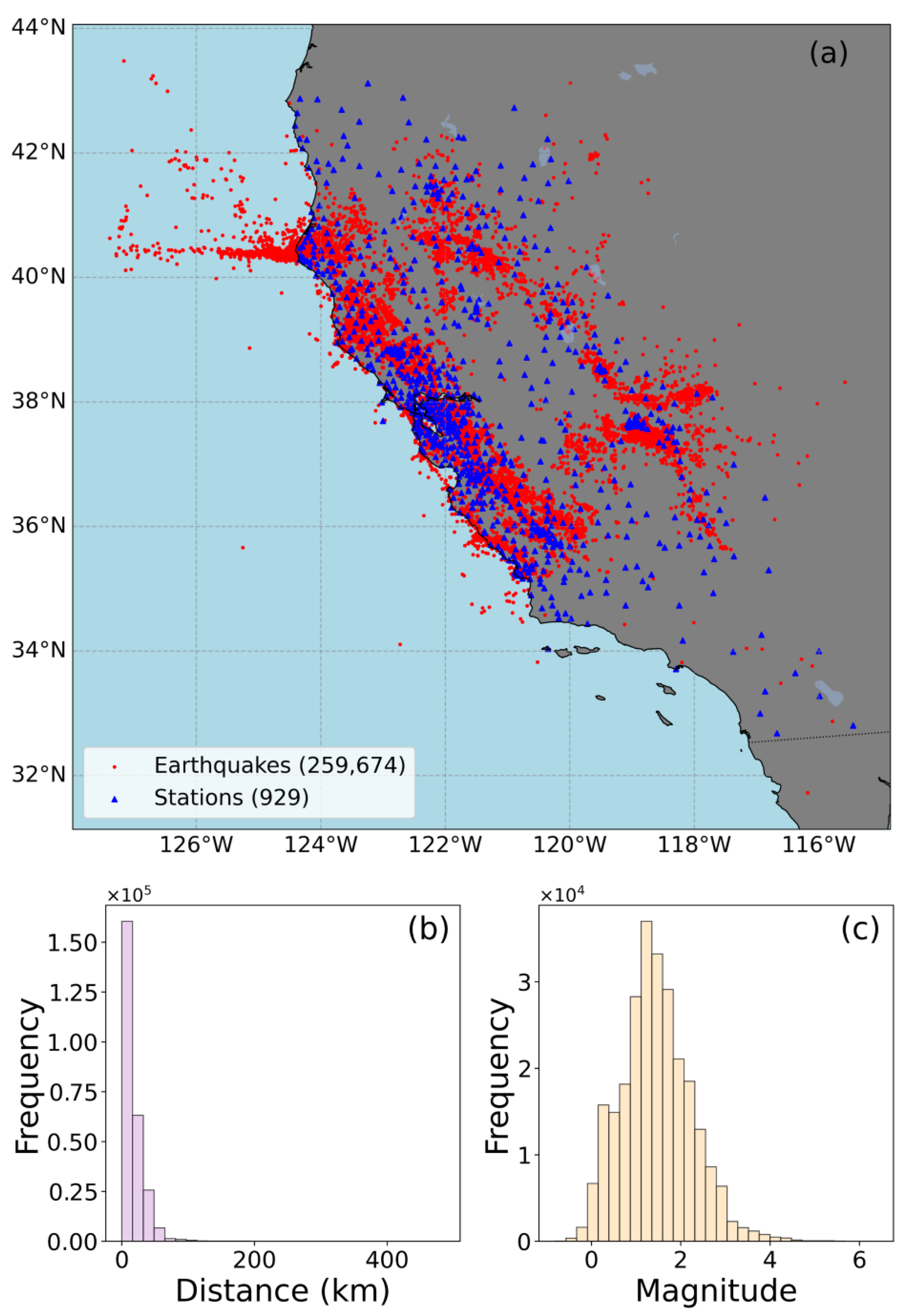
2. Data
3. Model
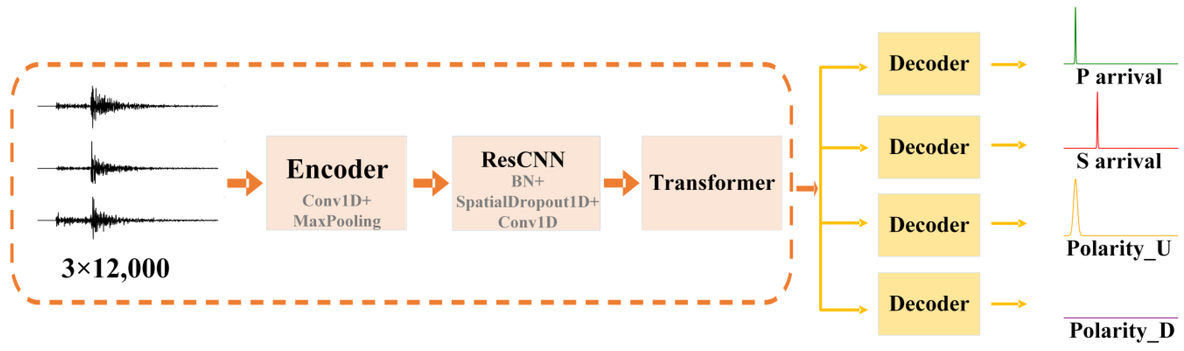
3.1. Model Building
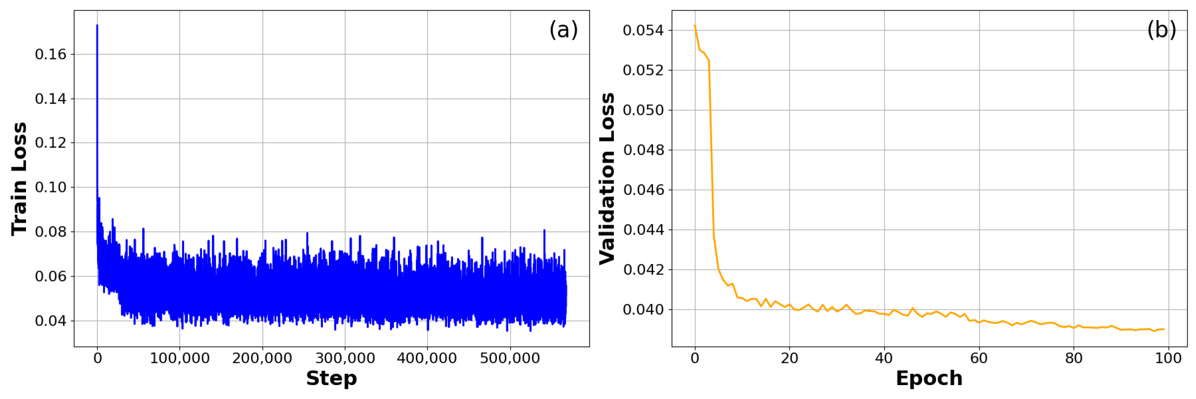
3.2. Model Training
4. Results
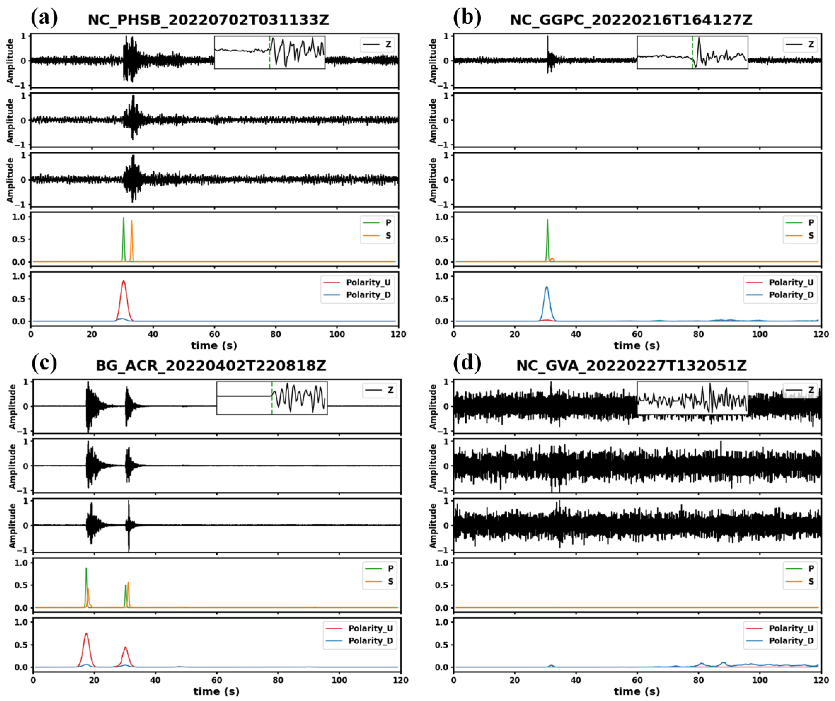
4.1. Test Set Analysis
4.2. The Geysers Dataset Analysis
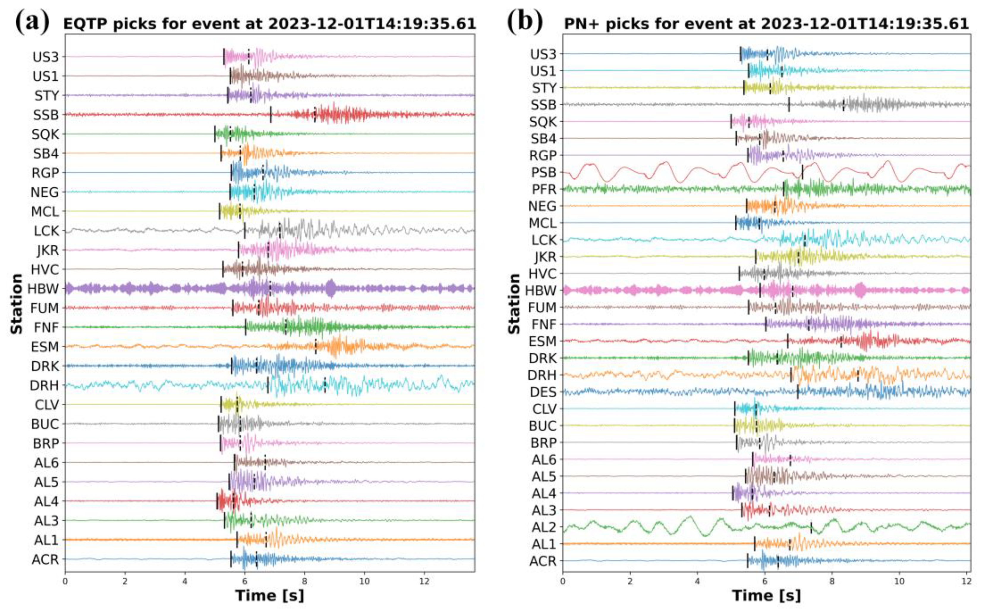
4.2.1. Phase Picking Analysis
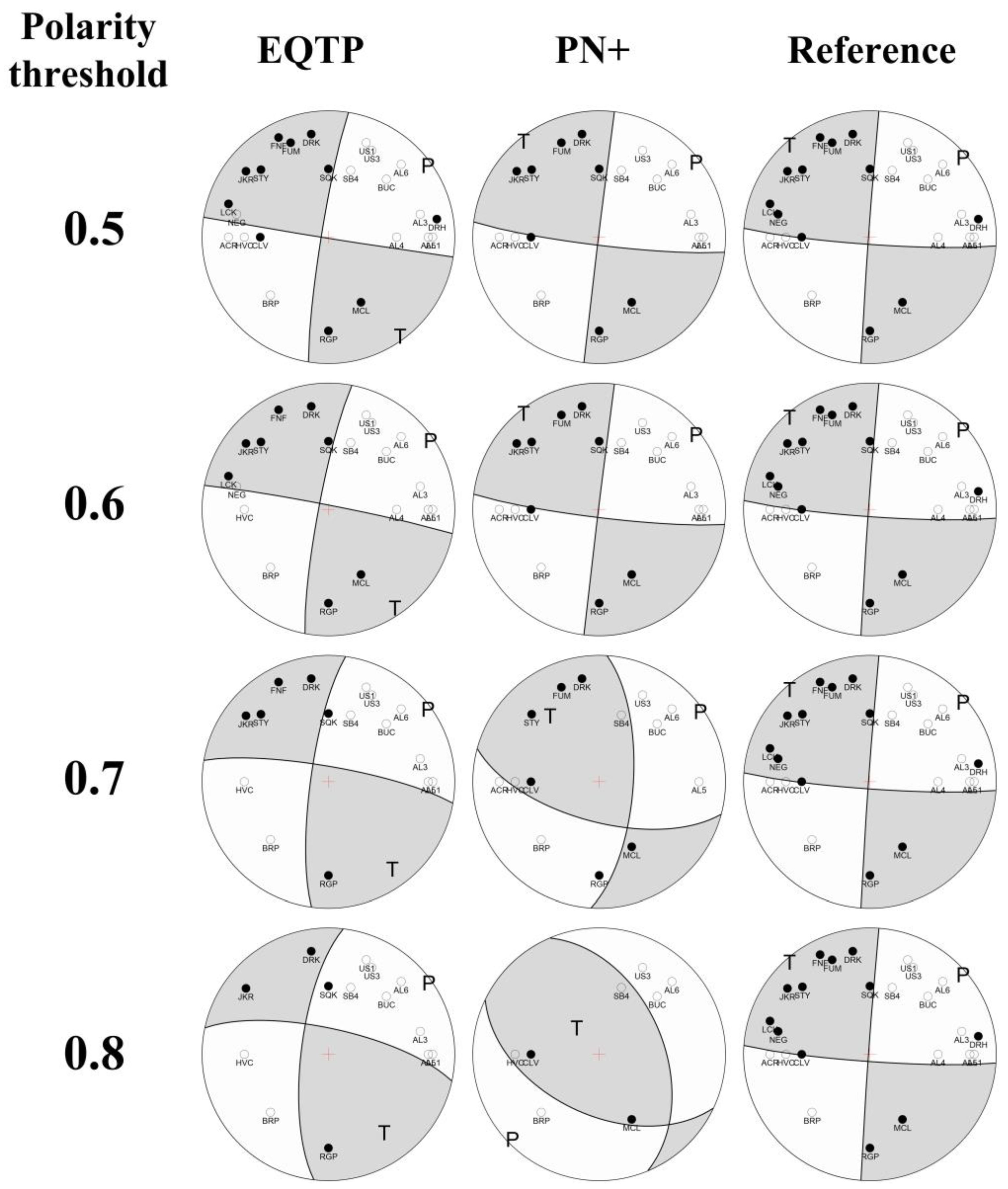
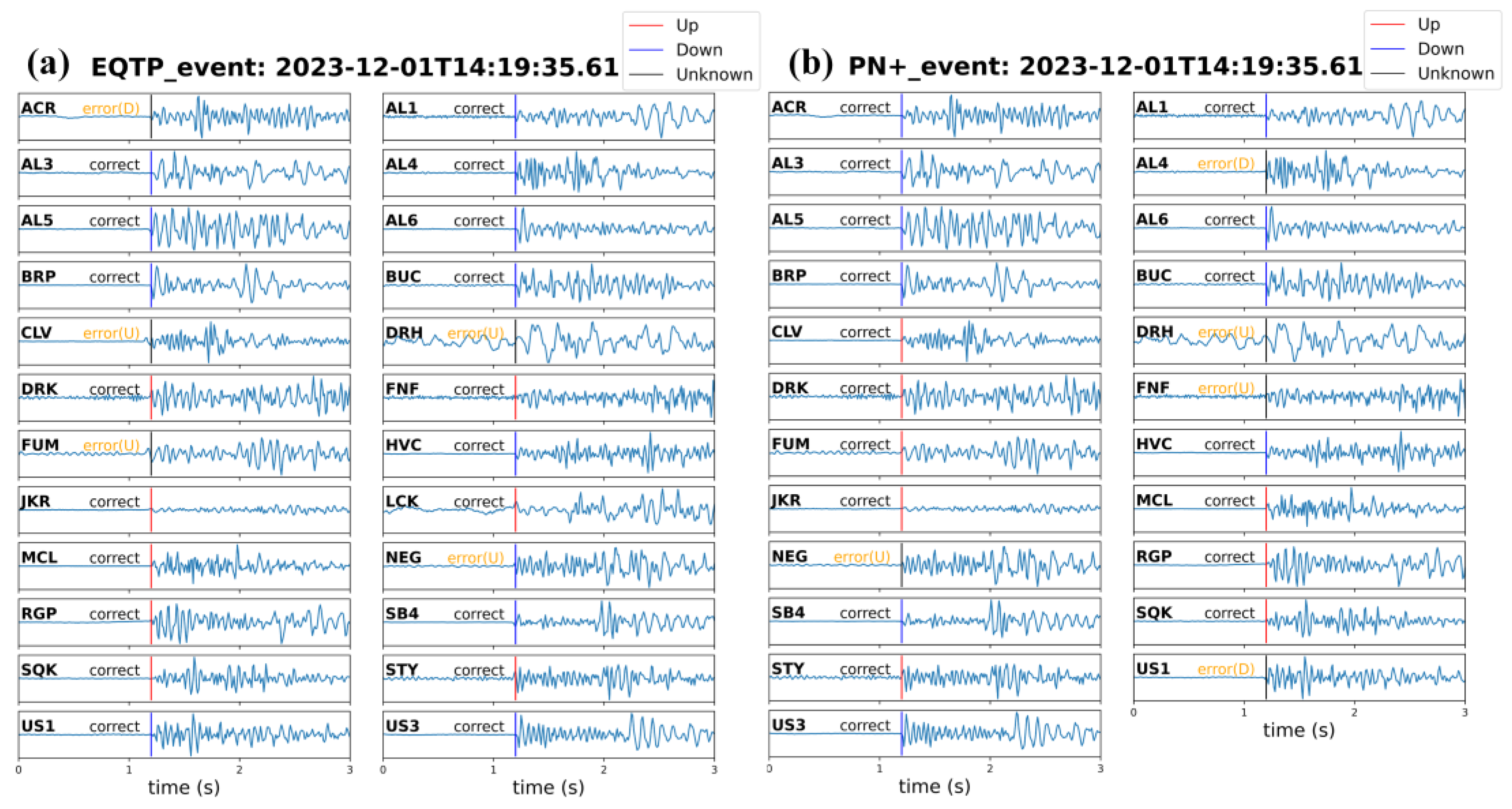
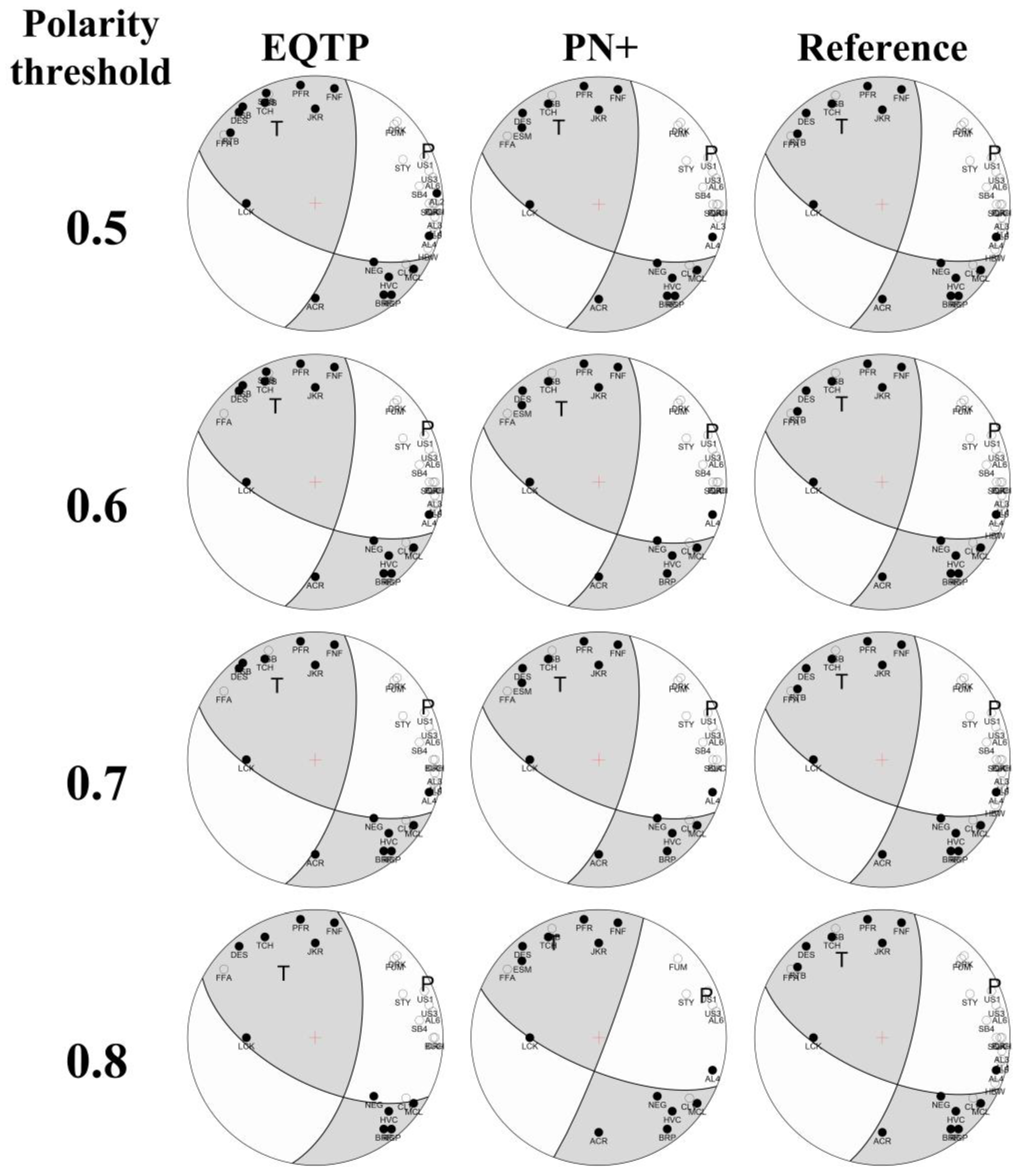
4.2.2. First-Arrival Polarity Determination Analysis
4.3. Generalization Ability Analysis
5. Discussion and Conclusions
Author Contributions
Funding
Institutional Review Board Statement
Informed Consent Statement
Data Availability Statement
Acknowledgments
Conflicts of Interest
References
- Eaton, D.W. Passive Seismic Monitoring of Induced Seismicity: Fundamental Principles and Application to Energy Technologies; Cambridge University Press: Cambridge, UK, 2018; ISBN 978-1-107-14525-2. [Google Scholar]
- Li, L.; Tan, J.; Wood, D.A.; Zhao, Z.; Becker, D.; Lyu, Q.; Shu, B.; Chen, H. A Review of the Current Status of Induced Seismicity Monitoring for Hydraulic Fracturing in Unconventional Tight Oil and Gas Reservoirs. Fuel 2019, 242, 195–210. [Google Scholar] [CrossRef]
- Li, L.; Tan, J.; Tan, Y.; Pan, X.; Zhao, Z. Chapter Eight—Microseismic Analysis to Aid Gas Reservoir Characterization. In Sustainable Geoscience for Natural Gas Subsurface Systems; Wood, D.A., Cai, J., Eds.; The Fundamentals and Sustainable Advances in Natural Gas Science and Eng; Gulf Professional Publishing: Houston, TX, USA, 2022; Volume 2, pp. 219–242. ISBN 978-0-323-85465-8. [Google Scholar]
- Xu, J.; Zhang, W.; Chen, X.; Guo, Q. An Effective Polarity Correction Method for Microseismic Migration-Based Location. Geophysics 2020, 85, KS115–KS125. [Google Scholar] [CrossRef]
- Barthwal, H.; van der Baan, M. Microseismicity Observed in an Underground Mine: Source Mechanisms and Possible Causes. Geomech. Energy Environ. 2020, 22, 100167. [Google Scholar] [CrossRef]
- Akaike, H. A New Look at the Statistical Model Identification. IEEE Trans. Autom. Control 1974, 19, 716–723. [Google Scholar] [CrossRef]
- Allen, R.V. Automatic Earthquake Recognition and Timing from Single Traces. Bull. Seismol. Soc. Am. 1978, 68, 1521–1532. [Google Scholar] [CrossRef]
- Pugh, D.J.; White, R.S.; Christie, P.A.F. Automatic Bayesian Polarity Determination. Geophys. J. Int. 2016, 206, 275–291. [Google Scholar] [CrossRef]
- Kim, J.; Woo, J.-U.; Rhie, J.; Kang, T.-S. Automatic Determination of First-Motion Polarity and Its Application to Focal Mechanism Analysis of Microseismic Events. Geosci. J. 2017, 21, 695–702. [Google Scholar] [CrossRef]
- Chen, C.; Holland, A.A. PhasePApy: A Robust Pure Python Package for Automatic Identification of Seismic Phases. Seismol. Res. Lett. 2016, 87, 1384–1396. [Google Scholar] [CrossRef]
- Tomassi, A.; de Franco, R.; Trippetta, F. High-Resolution Synthetic Seismic Modelling: Elucidating Facies Heterogeneity in Carbonate Ramp Systems. Pet. Geosci. 2025, 31, petgeo2024-47. [Google Scholar] [CrossRef]
- Anikiev, D.; Birnie, C.; bin Waheed, U.; Alkhalifah, T.; Gu, C.; Verschuur, D.J.; Eisner, L. Machine Learning in Microseismic Monitoring. Earth Sci. Rev. 2023, 239, 104371. [Google Scholar] [CrossRef]
- Lin, L.; Zhong, Z.; Li, C.; Gorman, A.; Wei, H.; Kuang, Y.; Wen, S.; Cai, Z.; Hao, F. Machine Learning for Subsurface Geological Feature Identification from Seismic Data: Methods, Datasets, Challenges, and Opportunities. Earth Sci. Rev. 2024, 257, 104887. [Google Scholar] [CrossRef]
- Yu, S.; Ma, J. Deep Learning for Geophysics: Current and Future Trends. Rev. Geophys. 2021, 59, e2021RG000742. [Google Scholar] [CrossRef]
- Li, L.; Zeng, X.; Pan, X.; Peng, L.; Tan, Y.; Liu, J. Microseismic Velocity Inversion Based on Deep Learning and Data Augmentation. Appl. Sci. 2024, 14, 2194. [Google Scholar] [CrossRef]
- LeCun, Y.; Boser, B.; Denker, J.S.; Henderson, D.; Howard, R.E.; Hubbard, W.; Jackel, L.D. Backpropagation Applied to Handwritten Zip Code Recognition. Neural Comput. 1989, 1, 541–551. [Google Scholar] [CrossRef]
- Chen, Y.; Zhang, G.; Bai, M.; Zu, S.; Guan, Z.; Zhang, M. Automatic Waveform Classification and Arrival Picking Based on Convolutional Neural Network. Earth Space Sci. 2019, 6, 1244–1261. [Google Scholar] [CrossRef]
- Dokht, R.M.H.; Kao, H.; Visser, R.; Smith, B. Seismic Event and Phase Detection Using Time–Frequency Representation and Convolutional Neural Networks. Seismol. Res. Lett. 2019, 90, 481–490. [Google Scholar] [CrossRef]
- Hara, S.; Fukahata, Y.; Iio, Y. P-Wave First-Motion Polarity Determination of Waveform Data in Western Japan Using Deep Learning. Earth Planets Space 2019, 71, 127. [Google Scholar] [CrossRef]
- Ross, Z.E.; Meier, M.-A.; Hauksson, E. P Wave Arrival Picking and First-Motion Polarity Determination with Deep Learning. J. Geophys. Res. Solid Earth 2018, 123, 5120–5129. [Google Scholar] [CrossRef]
- Tian, X.; Zhang, W.; Zhang, X.; Zhang, J.; Zhang, Q.; Wang, X.; Guo, Q. Comparison of Single-trace and Multiple-trace Polarity Determination for Surface Microseismic Data Using Deep Learning. Seismol. Res. Lett. 2020, 91, 1794–1803. [Google Scholar] [CrossRef]
- Uchide, T. Focal Mechanisms of Small Earthquakes beneath the Japanese Islands Based on First-Motion Polarities Picked Using Deep Learning. Geophys. J. Int. 2020, 223, 1658–1671. [Google Scholar] [CrossRef]
- Guo, T.Y.; Vanorio, T.; Ding, J. A Deep-Learning P-Wave Arrival Picker for Laboratory Acoustic Emissions: Model Training and Its Performance. Rock Mech. Rock Eng. 2024. [Google Scholar] [CrossRef]
- Shen, T.; Jiang, X.; Wang, S.; Peng, G. Improved U-Net3+ Network for First Arrival Picking of Noisy Earthquake Recordings. IEEE Trans. Geosci. Remote Sens. 2024, 62, 5912511. [Google Scholar] [CrossRef]
- Zhu, W.; Beroza, G.C. PhaseNet: A Deep-Neural-Network-Based Seismic Arrival Time Picking Method. Geophys. J. Int. 2019, 216, 261–273. [Google Scholar] [CrossRef]
- Chakraborty, M.; Cartaya, C.Q.; Li, W.; Faber, J.; Rümpker, G.; Stoecker, H.; Srivastava, N. PolarCAP—A Deep Learning Approach for First Motion Polarity Classification of Earthquake Waveforms. Artif. Intell. Geosci. 2022, 3, 46–52. [Google Scholar] [CrossRef]
- Vaswani, A.; Shazeer, N.; Parmar, N.; Uszkoreit, J.; Jones, L.; Gomez, A.N.; Kaiser, Ł.; Polosukhin, I. Attention Is All You Need. In Proceedings of the Advances in Neural Information Processing Systems; Curran Associates, Inc.: Newry, UK, 2017; Volume 30. [Google Scholar]
- Mousavi, S.M.; Ellsworth, W.L.; Zhu, W.; Chuang, L.Y.; Beroza, G.C. Earthquake Transformer—An Attentive Deep-Learning Model for Simultaneous Earthquake Detection and Phase Picking. Nat. Commun. 2020, 11, 3952. [Google Scholar] [CrossRef] [PubMed]
- Xiao, Z.; Wang, J.; Liu, C.; Li, J.; Zhao, L.; Yao, Z. Siamese Earthquake Transformer: A Pair-Input Deep-Learning Model for Earthquake Detection and Phase Picking on a Seismic Array. J. Geophys. Res. Solid Earth 2021, 126, e2020JB021444. [Google Scholar] [CrossRef]
- Zhao, M.; Xiao, Z.; Zhang, M.; Yang, Y.; Tang, L.; Chen, S. DiTingMotion: A Deep-Learning First-Motion-Polarity Classifier and Its Application to Focal Mechanism Inversion. Front. Earth Sci. 2023, 11, 1103914. [Google Scholar] [CrossRef]
- Li, S.; Fang, L.; Xiao, Z.; Zhou, Y.; Liao, S.; Fan, L. FocMech-Flow: Automatic Determination of P-Wave First-Motion Polarity and Focal Mechanism Inversion and Application to the 2021 Yangbi Earthquake Sequence. Appl. Sci. 2023, 13, 2233. [Google Scholar] [CrossRef]
- Chen, Y.; Saad, O.M.; Savvaidis, A.; Zhang, F.; Chen, Y.; Huang, D.; Li, H.; Aziz Zanjani, F. Deep Learning for P-Wave First-Motion Polarity Determination and Its Application in Focal Mechanism Inversion. IEEE Trans. Geosci. Remote Sens. 2024, 62, 5917411. [Google Scholar] [CrossRef]
- Chen, Y. Automatic Microseismic Event Picking via Unsupervised Machine Learning. Geophys. J. Int. 2020, 222, 1750–1764. [Google Scholar] [CrossRef]
- Li, H.; He, J.; Tuo, X.; Wen, X.; Yang, Z. Self-Supervised Convolutional Clustering for Picking the First Break of Microseismic Recording. IEEE Geosci. Remote Sens. Lett. 2024, 21, 7501105. [Google Scholar] [CrossRef]
- Mousavi, S.M.; Zhu, W.; Ellsworth, W.; Beroza, G. Unsupervised Clustering of Seismic Signals Using Deep Convolutional Autoencoders. IEEE Geosci. Remote Sens. Lett. 2019, 16, 1693–1697. [Google Scholar] [CrossRef]
- Zhang, J.; Li, Z.; Zhang, J. Simultaneous Seismic Phase Picking and Polarity Determination with an Attention-based Neural Network. Seismol. Res. Lett. 2023, 94, 813–828. [Google Scholar] [CrossRef]
- NCEDC. Northern California Earthquake Data Center. UC Berkeley Seismological Laboratory. Dataset 2014. [Google Scholar] [CrossRef]
- Zhu, W.; Wang, H.; Rong, B.; Yu, E.; Zuzlewski, S.; Tepp, G.; Taira, T.; Marty, J.; Husker, A.; Allen, R.M. California Earthquake Dataset for Machine Learning and Cloud Computing. arXiv 2025, arXiv:2502.11500. [Google Scholar]
- Martínez-Garzón, P.; Kwiatek, G.; Sone, H.; Bohnhoff, M.; Dresen, G.; Hartline, C. Spatiotemporal Changes, Faulting Regimes, and Source Parameters of Induced Seismicity: A Case Study from The Geysers Geothermal Field. J. Geophys. Res. Solid Earth 2014, 119, 8378–8396. [Google Scholar] [CrossRef]
- Yu, C.; Vavryčuk, V.; Adamová, P.; Bohnhoff, M. Moment Tensors of Induced Microearthquakes in The Geysers Geothermal Reservoir From Broadband Seismic Recordings: Implications for Faulting Regime, Stress Tensor, and Fluid Pressure. J. Geophys. Res. Solid Earth 2018, 123, 8748–8766. [Google Scholar] [CrossRef]
- Zhao, M.; Xiao, Z.; Chen, S.; Fang, L. DiTing: A Large-Scale Chinese Seismic Benchmark Dataset for Artificial Intelligence in Seismology. Earthq. Sci. 2023, 36, 84–94. [Google Scholar] [CrossRef]
- Woollam, J.; Münchmeyer, J.; Tilmann, F.; Rietbrock, A.; Lange, D.; Bornstein, T.; Diehl, T.; Giunchi, C.; Haslinger, F.; Jozinović, D.; et al. SeisBench—A Toolbox for Machine Learning in Seismology. Seismol. Res. Lett. 2022, 93, 1695–1709. [Google Scholar] [CrossRef]
- Yin, X.; Liu, Z.; Liu, D.; Ren, X. A Novel CNN-Based Bi-LSTM Parallel Model with Attention Mechanism for Human Activity Recognition with Noisy Data. Sci. Rep. 2022, 12, 7878. [Google Scholar] [CrossRef]
- Siami-Namini, S.; Tavakoli, N.; Namin, A.S. The Performance of LSTM and BiLSTM in Forecasting Time Series. In Proceedings of the 2019 IEEE International Conference on Big Data (big Data), Los Angeles, CA, USA, 9–12 December 2019; pp. 3285–3292. [Google Scholar]
- Sun, J.; Zhang, X.; Wang, J. Lightweight Bidirectional Long Short-Term Memory Based on Automated Model Pruning with Application to Bearing Remaining Useful Life Prediction. Eng. Appl. Artif. Intell. 2023, 118, 105662. [Google Scholar] [CrossRef]
- Bashir, T.; Wang, H.; Tahir, M.; Zhang, Y. Wind and Solar Power Forecasting Based on Hybrid CNN-ABiLSTM, CNN-Transformer-MLP Models. Renew. Energy 2025, 239, 122055. [Google Scholar] [CrossRef]
- Choi, Y.; Nguyen, H.-T.; Han, T.H.; Choi, Y.; Ahn, J. Sequence Deep Learning for Seismic Ground Response Modeling: 1D-CNN, LSTM, and Transformer Approach. Appl. Sci. 2024, 14, 6658. [Google Scholar] [CrossRef]
- Niksejel, A.; Zhang, M. OBSTransformer: A Deep-Learning Seismic Phase Picker for OBS Data Using Automated Labelling and Transfer Learning. Geophys. J. Int. 2024, 237, 485–505. [Google Scholar] [CrossRef]
- Shi, P.; Meier, M.-A.; Villiger, L.; Tuinstra, K.; Selvadurai, P.A.; Lanza, F.; Yuan, S.; Obermann, A.; Mesimeri, M.; Münchmeyer, J.; et al. From Labquakes to Megathrusts: Scaling Deep Learning Based Pickers over 15 Orders of Magnitude. J. Geophys. Res. Mach. Learn. Comput. 2024, 1, e2024JH000220. [Google Scholar] [CrossRef]
- Youden, W.J. Index for Rating Diagnostic Tests. Cancer 1950, 3, 32–35. [Google Scholar] [CrossRef]
- Zhu, W.; McBrearty, I.W.; Mousavi, S.M.; Ellsworth, W.L.; Beroza, G.C. Earthquake Phase Association Using a Bayesian Gaussian Mixture Model. J. Geophys. Res. Solid Earth 2022, 127, e2021JB023249. [Google Scholar] [CrossRef]
- Waldhauser, F. A Double-Difference Earthquake Location Algorithm: Method and Application to the Northern Hayward Fault, California. Bull. Seismol. Soc. Am. 2000, 90, 1353–1368. [Google Scholar] [CrossRef]
- Kwiatek, G.; Martínez-Garzón, P.; Bohnhoff, M. HybridMT: A MATLAB/Shell Environment Package for Seismic Moment Tensor Inversion and Refinement. Seismol. Res. Lett. 2016, 87, 964–976. [Google Scholar] [CrossRef]
- Celli, N.L.; Nooshiri, N.; Bean, C.J.; Grigoli, F.; Obermann, A.; Wiemer, S. Manual MT Inversions in Microseismic Areas: Good Practices and Building a Reference Database for the Hengill Region, Iceland. In Proceedings of the EGU General Assembly Conference Abstracts, Vienna, Austria, 23–27 May 2022; p. EGU22-11721. [Google Scholar]
- Kazemi, F.; Asgarkhani, N.; Jankowski, R. Optimization-Based Stacked Machine-Learning Method for Seismic Probability and Risk Assessment of Reinforced Concrete Shear Walls. Expert Syst. Appl. 2024, 255, 124897. [Google Scholar] [CrossRef]


| U | D | |
|---|---|---|
| U-pre | 18,865 | 2196 |
| D-pre | 1856 | 16,748 |
| N-pre | 97 | 79 |
| Total | 20,818 | 19,023 |
| Precision | Recall | F1 | Mean(s) | Std(s) | MAE(s) | Precision (Polarity) | Recall (Polarity) | F1 (Polarity) | |
|---|---|---|---|---|---|---|---|---|---|
| P | 1.00 | 1.00 | 1.00 | 0.00 | 0.05 | 0.02 | 0.90 | 0.89 | 0.90 |
| S | 1.00 | 0.99 | 1.00 | 0.01 | 0.15 | 0.09 |
| U | D | |
|---|---|---|
| U-pre | 30,485 (29,398) | 2113 (1672) |
| D-pre | 863 (1150) | 19,960 (19,588) |
| N-pre | 100 (783) | 137 (876) |
| Total | 31,448 (31,331) | 22,210 (22,136) |
| Precision | Recall | F1 | Mean(s) | Std(s) | MAE(s) | Precision (Polarity) | Recall (Polarity) | F1 (Polarity) | |
|---|---|---|---|---|---|---|---|---|---|
| P | 1.00 (1.00) | 0.99 (0.88) | 1.00 (0.94) | 0.01 (−0.01) | 0.05 (0.05) | 0.03 (0.03) | 0.94 (0.95) | 0.94 (0.92) | 0.94 (0.93) |
| S | 1.00 (1.00) | 0.97 (0.80) | 0.98 (0.89) | 0.04 (0.04) | 0.20 (0.17) | 0.12 (0.10) |
Disclaimer/Publisher’s Note: The statements, opinions and data contained in all publications are solely those of the individual author(s) and contributor(s) and not of MDPI and/or the editor(s). MDPI and/or the editor(s) disclaim responsibility for any injury to people or property resulting from any ideas, methods, instructions or products referred to in the content. |
© 2025 by the authors. Licensee MDPI, Basel, Switzerland. This article is an open access article distributed under the terms and conditions of the Creative Commons Attribution (CC BY) license (https://creativecommons.org/licenses/by/4.0/).
Share and Cite
Peng, L.; Li, L.; Zeng, X. A Microseismic Phase Picking and Polarity Determination Model Based on the Earthquake Transformer. Appl. Sci. 2025, 15, 3424. https://doi.org/10.3390/app15073424
Peng L, Li L, Zeng X. A Microseismic Phase Picking and Polarity Determination Model Based on the Earthquake Transformer. Applied Sciences. 2025; 15(7):3424. https://doi.org/10.3390/app15073424
Chicago/Turabian StylePeng, Ling, Lei Li, and Xiaobao Zeng. 2025. "A Microseismic Phase Picking and Polarity Determination Model Based on the Earthquake Transformer" Applied Sciences 15, no. 7: 3424. https://doi.org/10.3390/app15073424
APA StylePeng, L., Li, L., & Zeng, X. (2025). A Microseismic Phase Picking and Polarity Determination Model Based on the Earthquake Transformer. Applied Sciences, 15(7), 3424. https://doi.org/10.3390/app15073424