A Novel Optimal Control Strategy of Four Drive Motors for an Electric Vehicle

Abstract

Based on the mobility requirements of electric vehicles, four-wheel drive (4WD) can significantly enhance driving capability and increase operational flexibility in handling. If the output of different drive motors can be effectively controlled, energy losses during the distribution process can be reduced, thereby greatly improving overall efficiency. This study presents a simulation platform for an electric vehicle with four motors as power sources. This platform also consists of the driving cycle, driver, lithium-ion battery, vehicle dynamics, and energy management system models. Two rapid-prototyping controllers integrated with the required circuit to process analog-to-digital signal conversion for input and output are utilized to carry out a hardware-in-the-loop (HIL) simulation. The driving cycle, called NEDC (New European Driving Cycle), and FTP-75 (Federal Test Procedure 75) are used for evaluating the performance characteristics and response relationship among subsystems. A control strategy, called ECMS (Equivalent Consumption Minimization Strategy), is simulated and compared with the four-wheel average torque mode. The ECMS method considers different demanded powers and motor speeds, evaluating various drive motor power distribution combinations to search for motor power consumption and find the minimum value. As a result, it can identify the global optimal solution. Simulation results indicate that, compared to the average torque mode and rule-based control, in the pure simulation environment and HIL simulation during the UDDS driving cycle, the maximum improvement rates for pure electric energy efficiency for the 45 kW and 95 kW power systems are 6.1% and 6.0%, respectively. In the HIL simulation during the FTP-75 driving cycle, the maximum improvement rates for pure electric energy efficiency for the 45 kW and 95 kW power systems are 5.1% and 4.8%, respectively.

1. Introduction

The benefits of replacing petroleum fuel with electric power include environmental, economic, and energy security aspects [1]. Electric power can be generated from renewable sources, such as solar, wind, and hydropower, which can significantly reduce carbon emissions and help mitigate climate change issues [2]. Using electric power instead of petroleum can reduce the emission of nitrogen oxides, sulfur oxides, and particulates [3]. Equipment powered by electricity typically has lower operating costs than those driven by petroleum fuels due to their more stable electricity prices and less maintenance required [4]. Electricity can be produced from various sources, including nuclear, renewable energy, and fossil fuels, and this diversity reduces the risk of disruption in single-source energy supply [5]. Vehicles that currently use electric power as their primary energy source include pure electric cars, fuel cell vehicles, etc. Electric vehicles use motors with high energy conversion efficiency as their power source, have no exhaust emissions, and are generally considered the optimal mode of transportation in all sectors. However, they have disadvantages, such as low range and inconvenient charging [6]. The significant increase in various types of electric vehicles has led to the emergence of multiple electric vehicle structures, electric vehicle charging infrastructure, electric vehicles based on renewable energy, and integrated electric vehicle systems with the grid. To effectively manage the charging process, unique control strategies and power management strategies need to be implemented for multi-source electric vehicle systems [7]. However, the use of electric vehicles has some disadvantages, such as a limited battery range, a relatively short battery life, and a lack of existing electric vehicle charging infrastructure [8].

Based on previous studies, the optimization of hybrid energy/power systems primarily aims at energy conservation and cost reduction to achieve higher overall efficiency and enhance the overall system’s power [9]. Therefore, energy management strategies and the design of electric/power systems are two primary considerations. To obtain the optimal energy management strategy, rule-based control (RBC) is widely used in hybrid power systems [10]. This method is characterized by its ease of implementation, high computational efficiency, and rapid experimental verification. However, it inherently has the drawbacks of complex or highly nonlinear systems, limited to engineering intuitive design. To address such issues and enhance robustness, given the system’s uncertainties, fuzzy logic control (FLC) is suitable for various types of hybrid power systems [11,12]. The optimization can be carried out in parallel hybrid vehicles using dynamic programming algorithms and by designing driving cycles to determine the optimal hybridization factor and evaluate parameter sensitivity [13]. Dynamic programming has been widely referenced in numerous studies on hybrid vehicles and aircraft. It can determine the optimal trajectory by backtracking along the relationship between global power demand and time [14].

However, in systems with many control variables, a large number of logic rules may be required. Rule-based control can easily integrate global search results and verify controls with system variables. To overcome the quantitative analysis disadvantages derived from rule-based control, the concept of equivalent consumption minimization strategies (ECMS) is used to search for the best control (electric/power) source globally [15]. The ECMS requires dynamic calculations based on real-time data, which introduces significant computational complexity, increases the load on the controller, and demands higher hardware specifications. Under conditions of high-frequency operational changes, this computational load becomes particularly evident [16].

Using system simulation results presented in a multi-dimensional lookup table format and through program coding and direct downloading to the control unit, the ECMS design concept can be applied to energy management strategies and electric/power systems, further saving the power consumption of hybrid motorcycles and offering more rigorous academic analysis. The control objective can target energy efficiency and braking energy recovery performance, such as front and rear wheel braking torque distribution and hydraulic wheel-in motor braking energy recovery [17]. In the study of plug-in hybrid vehicles, the optimization goal is to minimize the vehicle’s instantaneous comprehensive operating costs. This involves integrating heterogeneous energy costs such as instantaneous engine fuel costs, battery electricity costs, and even battery aging costs into the objective function. An energy management control strategy is formulated to address the optimal gear-shifting problem and the optimal torque distribution problem [18]. The ECMS can convert the electrical energy of the battery into an equivalent amount of fuel consumption by introducing an Equivalent Factor for hybrid vehicles and minimizing the total fuel consumption at each moment. This total fuel consumption is the sum of the actual fuel consumption of the internal combustion engine and the weighted equivalent fuel consumption of the electric motor [19]. Therefore, the ECMS method is based on the principle that for the cost of energy distribution, the stored electrical energy is equivalent to consuming (or saving) a certain amount of fuel. Although this cost cannot be directly known because it depends on future vehicle behavior, it has been proven to be broadly related to driving conditions [20]. Additionally, the dual motor drive braking energy recovery technology first optimizes the charging efficiency, establishing the optimal distribution strategy of the front and rear motor braking torques under different driving modes, and verifies methods comparing rules based on the model predictive control using the hardware-in-the-loop (HIL) platform for verification [21].

Energy management is a crucial control technology for multiple energy sources. To fully utilize the energy-saving potential of four-wheel drive (4WD) electric vehicles, energy management strategies need to consider various constraints, such as the powertrain, driving conditions, and vehicle operational status, and balance the control’s economic and real-time aspects [22]. In 4WD electric vehicles, the power output of the front and rear motors directly affects the vehicle’s economy under different driving and braking conditions. ECMS implements various solutions for controlling the energy distribution of the front and rear motors under different driving conditions, with the primary goal of optimizing economy [23]. From the literature review, it can be concluded that the study mainly focuses on any type of 4WD electric vehicle architecture. The purpose of studying its performance is to optimize key aspects of HEV functionality, such as fuel reduction techniques. Energy management and power optimization are other important areas of focus [24]. In this study, actual vehicle controllers are applied, considering the improvement of computational efficiency and quantitative control analysis, adopting research and discussion on the four-wheel average torque mode and ECMS, and designing for four-wheel drive motor vehicles. In the ECMS method, a cost function is set, which here refers to the minimum total consumption of the four-wheel drive motors under test conditions; penalties are also set as well as the relationship between optimal search inputs and outputs [25]. The multi-power coupling system makes the energy management of 4WD electric vehicles relatively complex. To enhance vehicle economy and adaptability to driving modes, optimizing the energy management system is a critical factor [26]. Among them, the four drive motors serve as power sources, building a simulation platform for electric vehicles with four-wheel-side motors, using HIL simulation as an effective testing method, and exploring various vehicle data and performance metrics.

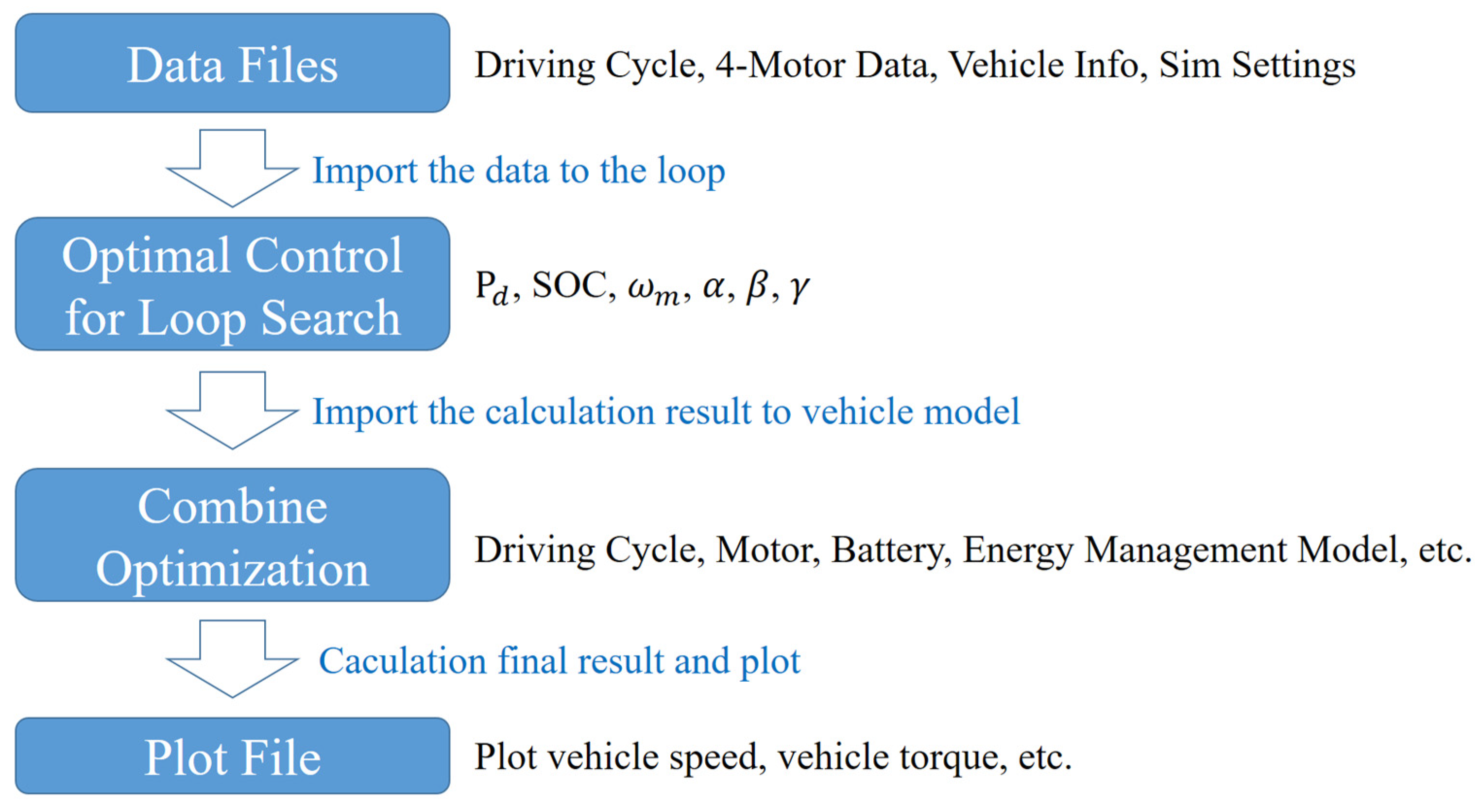
2. Simulation Platform and Optimal Energy Management

2.1. Electric Vehicle Simulation Platform

This study focuses on a four-wheel-side motor platform, choosing both the front and rear axles with independent suspension. A modified escape with a higher stance is selected. The drive motor chosen is the ZEPT 95 kW model with a gearbox [27], with the complete drive motor for mobile vehicles being provided by the complete electrification solution for mobile vehicles provided by the ZEPT (Zero Emission Power Train) company in Taoyuan City, Taiwan; the complete 288 V lithium battery system for mobile vehicles is provided by the National Chung-Shan Institute of Science and Technology in Taoyuan City, Taiwan, as shown in Figure 1.

Table 1. Specification of the electric vehicle.

Item		Specification
Drive Motor	Type	Permanent Magnet Synchronous
	Maximum Output Power	95 kW (Single)/380 kW (Four Units)
	Maximum Output Torque	210 Nm@4125 rpm
Energy Storage Battery	Type	Lithium-ion Ternary Battery
	Rated voltage	288 V
	Maximum Capacity	64.58 Ah (8.6 kWh)
Vehicle Parameters	Vehicle Mass	1728 kg
	Gravitational Acceleration	9.81 m/s2
	Aerodynamic Drag Coefficient	0.35
	Density of Air	1.2 kg/m3
	Frontal Area	3.5 m2
	Tire Radius	0.329 $\mathrm{m}$
	Rolling Resistance Coefficient	0.01
	Road Grade	0%
	Final Drive Ratio	9.78
	Drive Friction Coefficient	0.95

presents the specifications of the vehicle, including the drive motor, energy storage battery, and vehicle parameters used to facilitate energy efficiency calculations and performance analysis on the simulation platform.

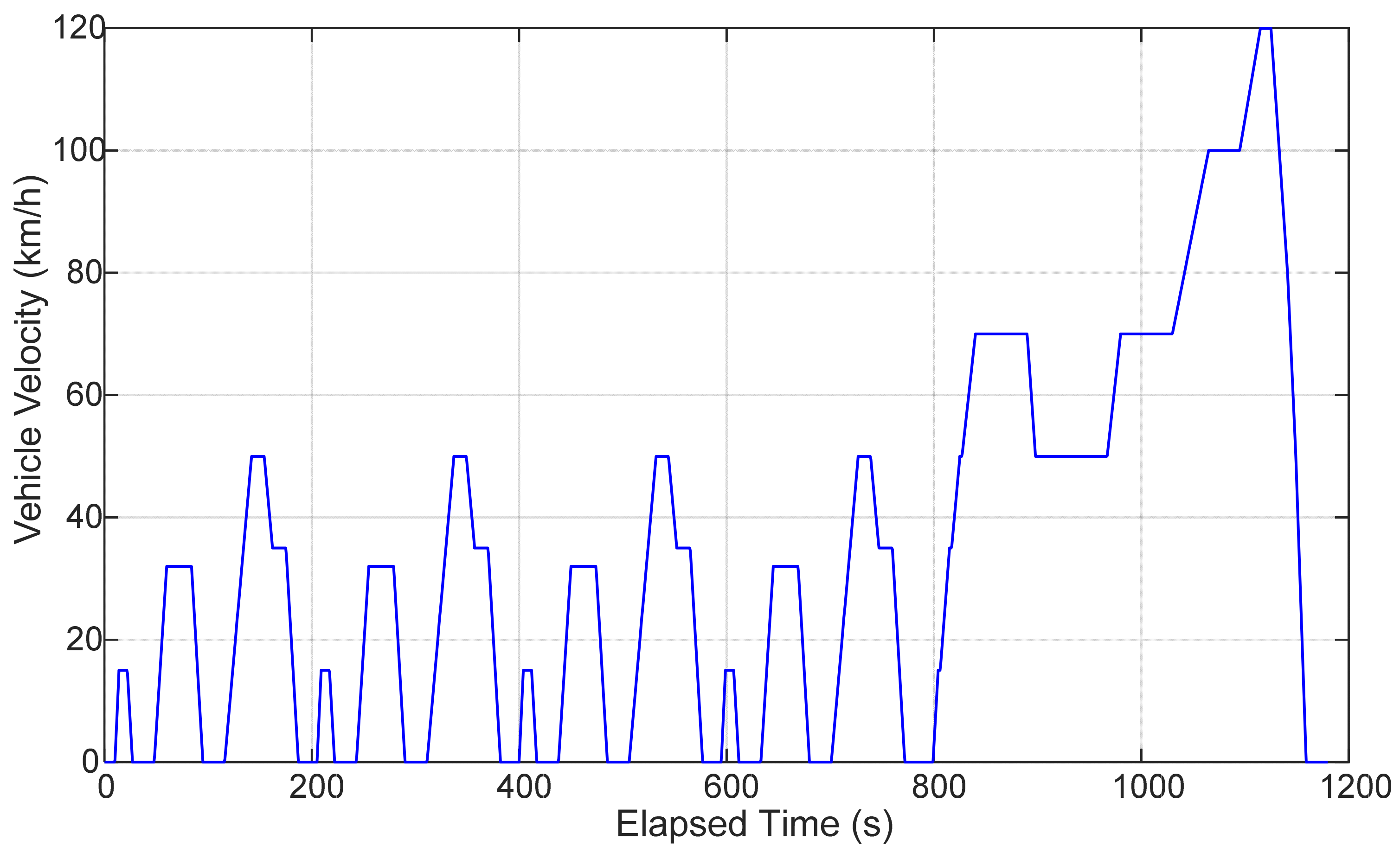
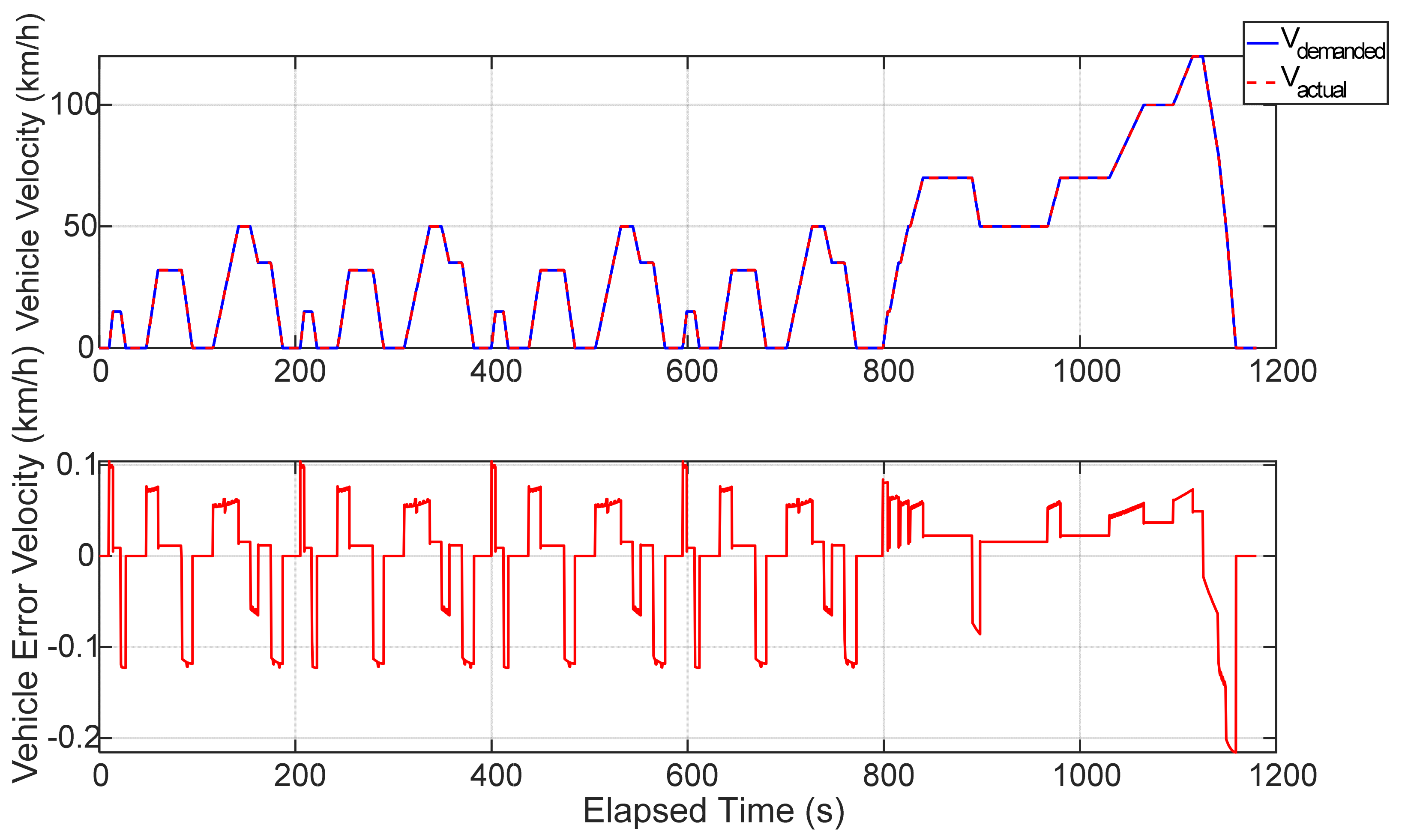
2.1.1. Driving Cycle Model

An important factor for consumers when purchasing an electric vehicle is its driving range. The driving range of an EV is determined by the total distance it can travel on a full charge until the battery is depleted. Currently, the mainstream energy consumption test standards for electric vehicles worldwide include the NEDC (New European Driving Cycle) and FTP-75 (Federal Test Procedure 75).

The NEDC is a commonly used automotive testing standard in Europe for assessing a vehicle’s fuel efficiency and emissions performance. This test cycle simulates urban and suburban driving conditions, as well as some high-speed situations [28]. The NEDC testing process includes fixed driving modes, speeds, and idle times, using these parameters to calculate the vehicle’s energy consumption. The total driving time is 1180 s, with a maximum vehicle velocity of 120 km/h. The overall vehicle velocity simulation is shown in Figure 2.

The FTP-75 is a standardized driving test cycle used for testing vehicle emissions, fuel economy, and energy consumption, established by the United States Environmental Protection Agency (EPA) [29]. This driving cycle is widely used in laboratory emission testing to simulate typical urban and highway mixed driving scenarios, and it provides experimental data to evaluate the environmental performance of vehicles. The driving time is 1370 s, with a maximum vehicle velocity of about 90 km/h. The overall vehicle velocity simulation is shown in Figure 3.

2.1.2. Driver Model

The driver model is responsible for simulating the control and response of the driver during acceleration and deceleration processes. This model uses a PI controller design and adjusts based on the difference between the demanded vehicle velocity and the actual vehicle velocity calculated by the whole vehicle simulation. The driver model takes the error between the demanded vehicle velocity and the actual vehicle velocity as the control signal to determine the demanded torque and brake torque. These output signals further adjust the total demanded torque of the entire vehicle, as shown in Formula (1):

$$T_d\left(t\right)={K_P·V}_{err}(t)+K_I·\int V_{err}\left(t\right)$$

(1)

where $T_d$ is the total demanded torque; $K_P$ is the proportional gain of the PI controller; $K_I$ is the integral gain of the PI controller; $V_{err}$ is the error between the demanded vehicle velocity and the actual vehicle velocity.

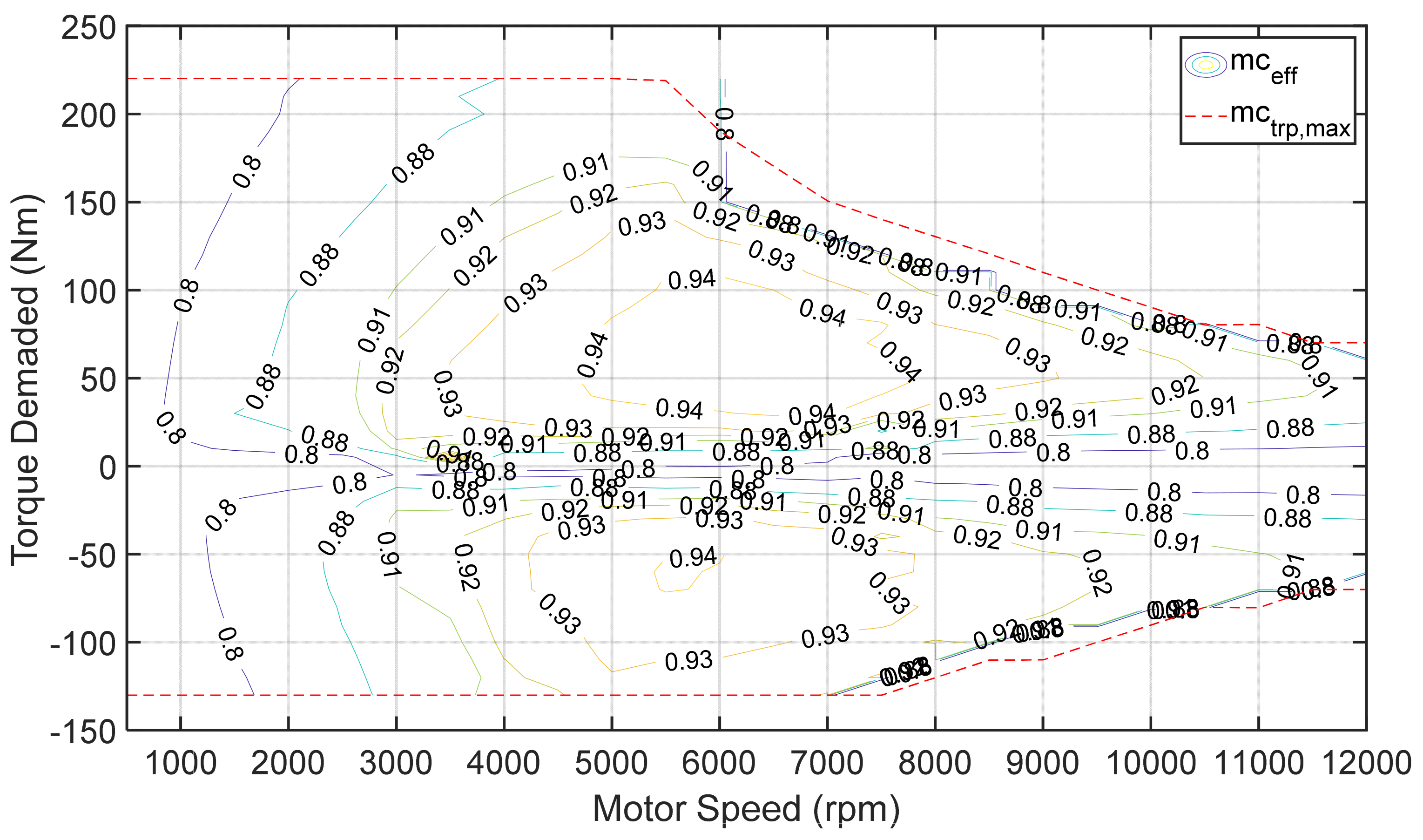
2.1.3. Drive Motor Model

In this study, the drive motor model, utilizing the demanded torque from the driver model, calculates the torque based on the maximum physical limit of the drive motor speed for protection. It then outputs the appropriate drive motor torque for propulsion. Figure 4 shows the mechanical efficiency curve of the drive motor, with test data provided by the ZEPT company, where the efficiency of the drive motor is determined based on the current speed and torque of the drive motor through a two-dimensional table. It is shown that at a torque of 60 Nm and a rotational speed of approximately 6500 rpm, the motor achieves a peak efficiency of 94.99%. At the same rotational speed, applying a negative input torque indicates that the motor is operating in generator mode. The motor efficiency is shown in Formula (2):

$${\eta }_m\left(t\right)=f(T_m\left(t\right), N_m(t\left)\right)$$

(2)

where ${\eta }_m$ is the efficiency of the drive motor; $T_m$ is the output torque of the drive motor; $N_m$ is the wheel speed of the drive motor.

2.1.4. Lithium Battery Model

The lithium battery pack serves as the power source for the vehicle’s drive motor. Based on data from ADVISOR^® (2002, NREL’s advanced vehicle simulator), a relationship between the lithium battery voltage and internal resistance is constructed, and the State of Charge (SOC) of the lithium battery is calculated based on the results obtained. Regarding the operating temperature of the lithium battery, this study’s model sets the battery temperature to a fixed value and does not consider changes in battery temperature under actual usage conditions, which would vary with usage conditions and operating time. The accuracy of lithium battery charge estimation impacts the overall vehicle dynamics and energy management strategies. Typically, the internal resistance is shown in Formula (3):

$$R_b=R_b({SOC}_b,t_b)$$

(3)

where $R_b$ is the equivalent internal resistance of the lithium battery; ${SOC}_b$ is the state of charge for the lithium battery; $t_b$ is the lithium battery temperature. SOC represents a range from 0 to 1 (0–100%), and its calculation method is shown in Formula (4):

$${SOC}_b={\displaystyle \frac{{SOC}_{int}Q-\int \frac{I_b}{{\eta }_b}dt}{Q}}$$

(4)

where $Q$ is the rated capacity of the lithium battery; $I_b$ is the discharge current of the lithium battery; ${\eta }_b$ is the charge-discharge efficiency of the lithium battery. ${\eta }_b$ is a function of the relationship between $V_{OC}$ and $I_b$:

$${\eta }_b={\eta }_b(V_{OC},I_b)$$

(5)

The discharge current of the lithium battery calculation method is as shown in Formula (6):

$$I_b={\displaystyle \frac{V_{OC}-\sqrt{{V_{OC}}^2-4\times P_b\times R_b}}{2\times R_b}}$$

(6)

where $V_{OC}$ is the open circuit voltage of the lithium battery, a function of ${SOC}_b$ and $I_b$; $P_b$ is the discharge power of the battery to the drive motor. The calculation method for the load voltage of the battery during discharge is shown in Formula (7):

$$V_b=V_{OC}-I_b\times R_b$$

(7)

The calculation of dynamic resistance performance uses the internal resistance method, which can be determined through experimental data on energy storage batteries, anticipating the change in internal resistance of each battery at different SOC levels, and obtaining the open circuit voltage values at various SOCs.

2.1.5. Vehicle Dynamics Model

The vehicle dynamics model needs to consider the impedance of various conditions while driving. The EV’s propulsion is equal to the sum of its drive force and the reverse force in the direction of travel. The main loads during bus operation include air resistance $R_a$, gradient resistance $R_g$, and rolling resistance $R_r$. Whenever a vehicle moves, it encounters resistance from the air, known as air resistance. This resistance increases proportionally to the square of the vehicle’s velocity, shown in Formula (8):

$$R_a={\displaystyle \frac{1}{2}}{\rho }_a{C}_d{A}_f{V_{\mathit{veh}}}^2$$

(8)

where $R_a \mathrm{i}\mathrm{s} \mathrm{t}\mathrm{h}\mathrm{e} \mathrm{a}\mathrm{i}\mathrm{r} \mathrm{r}\mathrm{e}\mathrm{s}\mathrm{i}\mathrm{s}\mathrm{t}\mathrm{a}\mathrm{n}\mathrm{c}\mathrm{e}; C_d$ is the drag coefficient; $A_f$ is the frontal area of the EV; ${\rho }_a$ is the air density; $V_{veh}$ is the vehicle velocity.

Rolling resistance refers to the energy lost when a tire rolls. This energy loss is primarily due to the continuous deformation of the tire. Additionally, due to road surface irregularities, the tire experiences longitudinal forces that contribute to rolling resistance, as shown in Formula (9):

$$R_r=\mu m_{\mathit{veh}}g\cos \left(\theta \right)$$

(9)

where $R_r$ is the rolling resistance; $m_{veh}$ is the total vehicle mass; $\mu$ is the rolling resistance coefficient; $g$ is the gravitational acceleration.

The resistance a vehicle encounters when ascending a slope is referred to as gradient resistance, as indicated by Formula (10):

$$R_g=m_{\mathit{veh}}g\sin \left(\theta \right)$$

(10)

where $R_g$ is the gradient resistance.

Which has a significant impact while driving. Ultimately, the drive wheel speed and actual vehicle velocity will be calculated, and the results will be fed back to the driver model and used for overall vehicle torque control. The vehicle’s acceleration force is equal to the drive force minus $R_a$, $R_r$ $R_g$, and the braking force, as shown in Formula (11):

$$m_{veh}{\displaystyle \frac{d{V}_{veh}}{dt}}={\displaystyle \frac{T_f{\eta }_f}{r_w}}-R_a-R_r{-R}_g-F_{brk}$$

(11)

where $r_w$ is the tire radius; $T_f$ is the output torque of the final drive; ${\eta }_f$ is the overall efficiency of the final drive; $F_{brk}$ is the braking force; $\theta$ is the gradient angle.

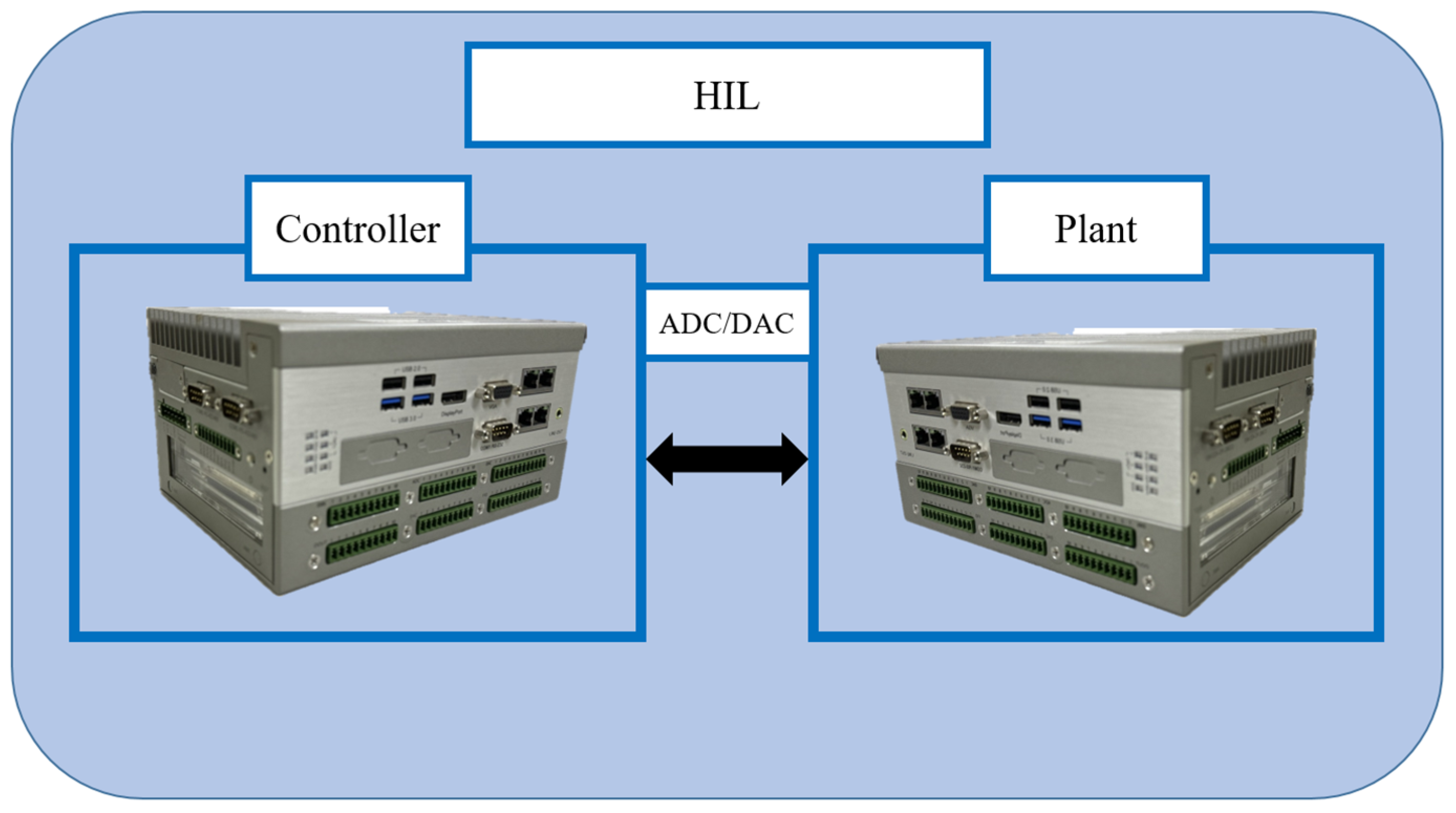
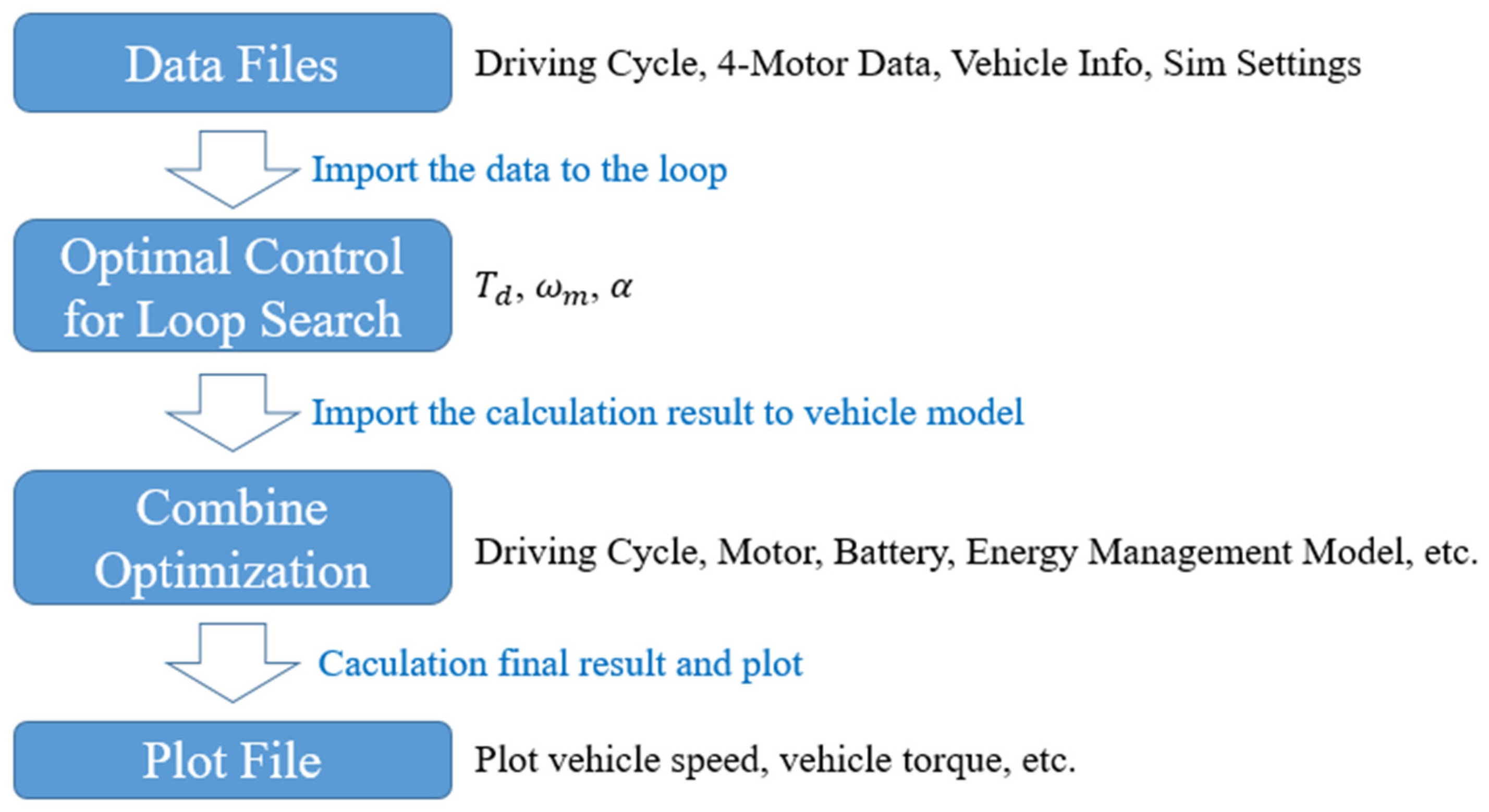
2.1.6. Hardware-in-the-Loop System Architecture

The HIL is a method used in the development of algorithms, where parameters from physical systems are input into a program, and various computational modules are constructed. This builds the physical models used in this research to test whether the control logic in the controller functions correctly under real-world conditions, and it can also reduce development costs [30]. This study employs the rapid prototyping controller (Micro-Box 2200^® /Terasoft, company in Hsinchu County, Taiwan) to construct a HIL system platform, providing a real-time model of the entire vehicle platform and its controller. This system requires capturing data from the entire vehicle to adapt to the construction of the HIL system. Starting with the initial driving cycle model, the demanded vehicle velocity is input into the driver model, and after PI computation, the total vehicle demanded torque is sent to the drive motor model. The vehicle dynamics model outputs the motor speed, which passes through the Energy Management System (EMS) model. The EMS allocates the output torque to the drive motor model based on control strategies and then sends it back to the receiving end of the Micro-Box 2200 rapid prototyping controller, as shown in Figure 5. During the signal transmission process between the vehicle system and the controller, the vehicle signal variables are continuously converted into voltage signals, which are then converted into the physical signals required by the vehicle, ensuring accurate signal transmission between the vehicle system and the controller. Simulations of various control strategies were conducted within both the Simulink environment and an HIL platform. Initially, the complete vehicle model was deployed onto the second hardware platform, functioning as the plant. This platform received voltage signals from the first hardware platform, converting analog voltages into digital signals. After computations within the vehicle model, the demanded power and actual motor speed were converted between digital and analog forms, transforming physical quantities into voltage signals sent back to the first hardware platform. At this stage, the first platform acted as the controller, executing control strategy calculations. Upon receiving analog voltage signals, it immediately converted them into digital signals, performed control strategy computations, and translated various motor torque demands from physical quantities into analog voltage signals, transmitting them to the second hardware platform. Finally, by inputting the NEDC or FTP-75 driving cycles, real-time tests demonstrated the proposed optimization strategy’s high applicability in online energy management.

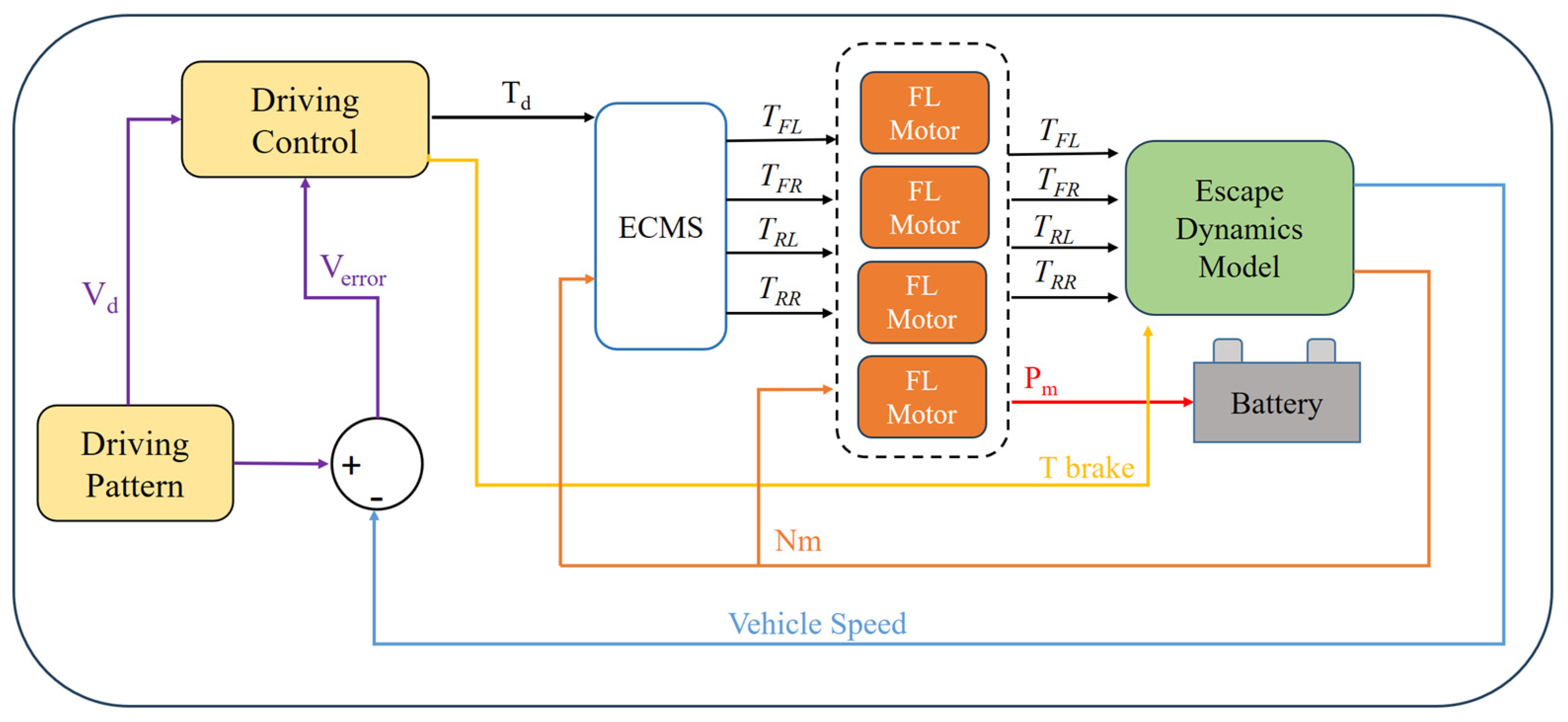
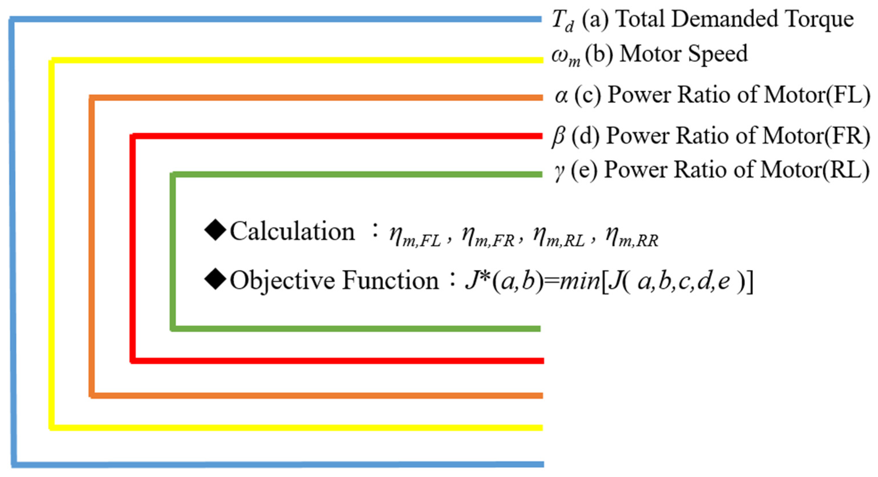
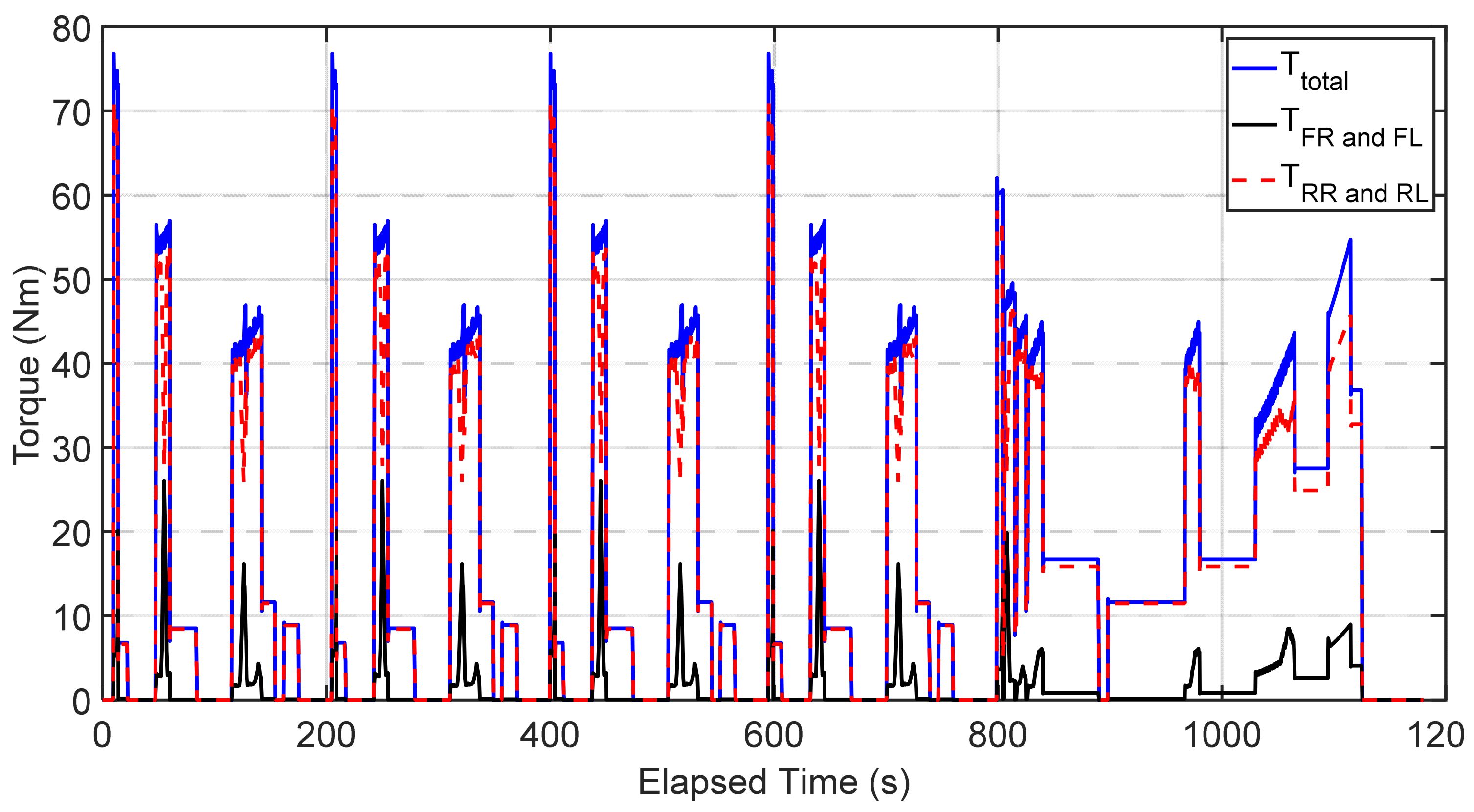
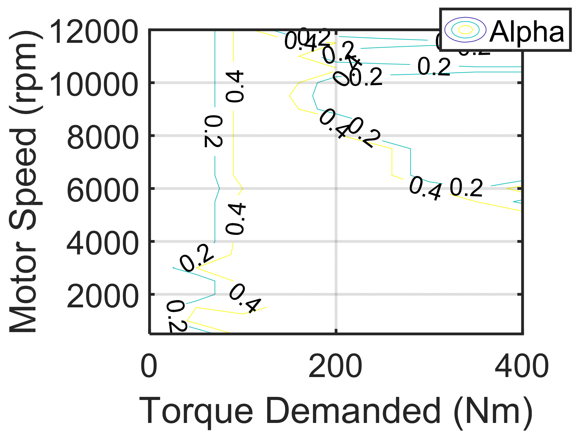
2.2. Optimal Energy Management of the Four-Wheel-Side Motors

The resolution of the ECMS method is limited by the size of the grid established and the hardware equipment used. If the range between the parameter grids is too large, the conditions calculated may not precisely fall on the grid points of the multi-dimensional table. In such cases, the solution for that condition will be obtained using the built-in interpolation method within the system. By using this method and considering all factors in the search, it is possible to find the global optimum solution. Based on the optimal efficiency method of four-wheel-side motors, this study applies the ECMS theory to obtain the optimal power distribution ratio (PR), presenting the battery power variation in the form of equivalent fuel consumption. The vehicle specifications are shown in Table 1. The simulated whole-vehicle structure diagram is shown in Figure 6. The demanded vehicle velocity is first provided by the driving mode model. The actual vehicle velocity is then calculated in the vehicle dynamics model. The difference in velocity between the two is determined to carry out PI control. In this setup, the PI controller controls the forward torque command to the energy management model for power distribution of the four-wheel-side motors. The negative torque command controls the brake torque to the vehicle dynamics model for vehicle braking. The energy management model calculates, based on the actual rotation speed of the vehicle dynamics model, using the optimal power distribution torque command to operate each motor. Finally, the output from the four-wheel-side motors is sent to the entire vehicle dynamics model for the actual vehicle velocity.

The output torque of the left front wheel motor is related to the demanded torque and varies linearly with the power distribution ratio of the first gear, as shown in Formula (12):

$$T_{m,FL}=\alpha \times T_d$$

(12)

where $T_{m,FL}$ is the output torque of the left front wheel motor; $\alpha$ is the power distribution ratio of the first gear; $T_d$ is the demanded torque.

The output torque of the right front wheel motor is related to the demanded torque and varies linearly with the power distribution ratio of the second gear, as shown in Formula (13):

$$T_{m,FR}=\beta \times T_d$$

(13)

where $T_{m,FR}$ is the output torque of the right front wheel motor; $\beta$ is the power distribution ratio of the second gear.

The output torque of the left rear wheel motor is related to the demanded torque and varies linearly with the power distribution ratio of the third gear, as shown in Formula (14):

$$T_{m,RL}=\gamma \times T_d$$

(14)

where $T_{m,RL}$ is the output torque of the left rear wheel motor; $\gamma$ is the power distribution ratio of the third gear.

The output torque of the right rear wheel motor is determined by subtracting the torques of the other three wheels from the total demanded torque, as indicated in Formula (15):

$$T_{m,RR}=\left(1-\alpha -\beta -\gamma \right)\times T_d$$

(15)

where $T_{m,RR}$ is the output torque of the right rear wheel motor.

Formulas (12)–(15) are consolidated into Formula (16):

$$T_{m,FL}+T_{m,FR}+T_{m,RL}+T_{m,RR}={\alpha T}_d+\beta T_d+\gamma T_d+T_d-\alpha T_d-\beta T_d-\gamma T_d$$

(16)

Formula (16) is derived by simplifying Formula (17):

$$T_d=T_{m,FL}+T_{m,FR}+T_{m,RL}+T_{m,RR}$$

(17)

Measurement data and physical constraint input: Data from real vehicle examples (Escape 2002) of four types of wheel-side motors and lithium battery groups were tested and needed to be imported into the program, formed into one-dimensional or two-dimensional tables. This included demanded torque, motor speed, and power distribution ratios. Limitations included the relationship between the maximum output torque and speed of the four-wheel-side motors. Based on the quantified data, optimization algorithms can be implemented. The program contains 5 “For Loops”, which globally search for discretized demanded torque, motor speeds, etc. Within the program, through “if-then-else” conditions, various possible operation modes are determined, followed by calculations of various parameters, such as the efficiency and torque of the four-wheel-side motors. Then, using the concept of equivalent fuel consumption, equivalent fuel consumption under various conditions can be calculated. Minimum fuel consumption results are obtained and stored in a two-dimensional matrix called “mf_total_boost”. Thus, by finding the minimum equivalent fuel consumption at fixed speeds and demanded torques and different torques of the four-wheel-side motors, the optimal power distribution ratio can be derived.

In the program calculation, the parameters for system model establishment, such as the efficiency of the four-wheel-side motors, the maximum torque limits of the four-wheel-side motors, and battery parameters, are included, and a control system’s optimal distribution model parameter analysis process is constructed. This effectively simplifies the control model to meet the real-time computing needs of embedded systems. To obtain the optimal control model parameters, a global search is used to find the best parameter solution. For instance, in four-wheel torque mode, the optimal power distribution control can first discretize (discretization) necessary input parameters, such as the demanded torque and motor speed. A target function is then established to obtain the optimal power distribution ratio through the ECMS algorithm. Calculate the power consumption of the four-wheel-side motors and find the minimum value; the cost function is as shown in Formula (18):

$$J=min({\dot{E}}_{m,FL}+{\dot{E}}_{m,FR}+{\dot{E}}_{m,RL}+{\dot{E}}_{m,RR}+\omega )$$

(18)

where ${\dot{E}}_{m,FL}$ is the input power of the left front wheel motor; ${\dot{E}}_{m,FR}$ is the input power of the right front wheel motor; ${\dot{E}}_{m,RL}$ is the input power of the left rear wheel motor; ${\dot{E}}_{m,RR}$ is the input power of the right rear wheel motor; $J$ is the optimal objective function; and $\omega$ represents the relationship between the battery SOC and the penalty value.

The output power calculation of the left front wheel motor is shown in Formula (19):

$${\dot{E}}_{m,FL}={\displaystyle \frac{T_{m,FL}\times N_m}{{\eta }_{m,FL}}}$$

(19)

where $N_m$ is the wheel speed (in rad/s) of the wheel-side motor; ${\eta }_{m,FL}$ is the efficiency of the left front wheel motor.

The output power calculation of the right front wheel motor is shown in Formula (20):

$${\dot{E}}_{m,FR}={\displaystyle \frac{T_{m,FR}\times N_m}{{\eta }_{m,FR}}}$$

(20)

where ${\eta }_{m,FR}$ is the efficiency of the right front wheel motor.

The output power calculation of the left rear wheel motor is shown in Formula (21):

$${\dot{E}}_{m,RL}={\displaystyle \frac{T_{m,RL}\times N_m}{{\eta }_{m,RL}}}$$

(21)

where ${\eta }_{m,RL}$ is the efficiency of the left rear wheel motor.

The output power calculation of the right rear wheel motor is shown in Formula (22):

$${\dot{E}}_{m,RR}={\displaystyle \frac{T_{m,RR}\times N_m}{{\eta }_{m,RR}}}$$

(22)

where ${\eta }_{m,RR}$ is the efficiency of the right rear wheel motor.

By substituting Formula (18) into Formulas (19)–(22), the cost function is as shown in Formula (23):

$$J=min ({\displaystyle \frac{T_{m,FL}\times N_m}{{\eta }_{m,FL}}}+{\displaystyle \frac{T_{m,FR}\times N_m}{{\eta }_{m,FR}}}+{\displaystyle \frac{T_{m,RL}\times N_m}{{\eta }_{m,RL}}}+{\displaystyle \frac{T_{m,RR}\times N_m}{{\eta }_{m,RR}}}+\omega )$$

(23)

When $\omega$ the conditions of a search grid exceed physical limits for the four-wheel-side motors, a very large value will be given:

$$\omega ={10}^6 \left(\mathit{Penalty}\right) \mathit{or} \omega =0 \left(\mathit{Normal}\right)$$

(24)

The system primarily needs to identify the motor’s equivalent fuel consumption minimization strategy, the $J$ function, and, based on this $J$ function strategy, determine the optimal motor equivalent energy consumption. The optimal energy distribution loop is shown in Figure 7. Discretized variables include the demanded torque, motor speed, power ratio of the left front wheel motor ($\alpha$), power ratio of the right front wheel motor ($\beta$), and power ratio of the left rear wheel motor ($\gamma$). These are used to conduct a global search, calculating the total electrical energy consumption or equivalent fuel consumption of the four-wheel-side motors under different variables. The development workflow is shown in Figure 8. Through a two-fold minimization using bilinear interpolation, based on the demanded torque and motor speed as a loop, the search for the lowest power consumption of the four-wheel-side motors can be performed. The cost function can be formulated in a matrix form as a two-dimensional optimization, as shown in Formula (25).

$$J^{*}(a,b)=min\left[J\left(a,b,c,d,e\right)\right]$$

(25)

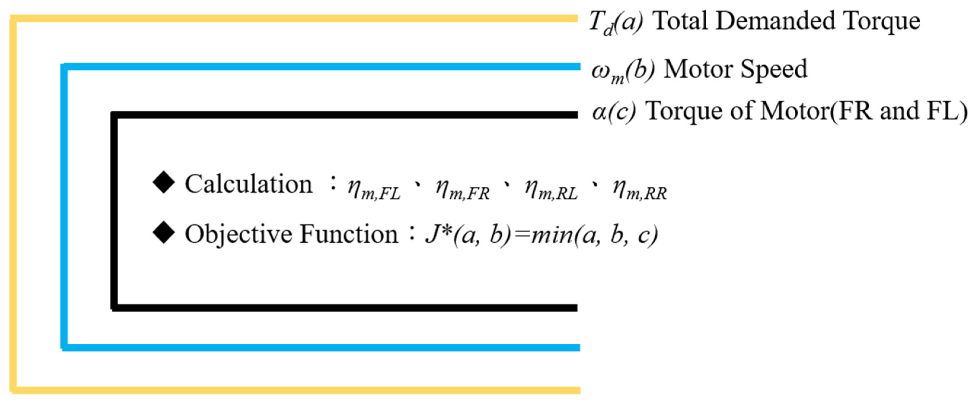
2.3. Optimal Energy Management of the Front and Rear Axle Motors

Due to the optimal energy distribution design of the four-wheel-side motors, during turning or straight-line driving, there is an uneven torque distribution among the four wheels. Through analysis using the CarSim vehicle dynamics software^® (2021, CarSim, Santa Clara County, CA, USA), a phenomenon of the vehicle “swaying” or “yawing” was observed [31,32]. Therefore, an optimal energy distribution design for the front and rear axle motors was established to improve this, as shown in Figure 9. A grid search based on the mechanical efficiency matrix of motor torque and speed ensures that the four-wheel-side motors can maintain the demanded power of the vehicle and operate all motors within their optimal efficiency ranges, achieving energy-saving effects. However, the optimal energy distribution design for the four-wheel-side motors can cause the vehicle to deviate from its ideal trajectory due to uneven torque distribution among the wheels during driving. Therefore, in subsequent designs, the optimal energy distribution design for the front and rear axle motors is used to address this issue. For definitions of related parameters, please refer to the description of the optimal energy distribution design for the front and rear axle motors. The revised formulas for various power distribution ratios are shown in

$$T_{m,FL}=T_{m,FR}={\displaystyle \frac{\alpha \times T_d}{2}}$$

(26)

$${T_{m,RL}=T}_{m,RR}={\displaystyle \frac{\left(1-\alpha \right)\times T_d}{2}}$$

(27)

$$T_{m,FL}+T_{m,FR}+T_{m,RL}+T_{m,RR}={\displaystyle \frac{\alpha \times T_d}{2}}+{\displaystyle \frac{\alpha \times T_d}{2}}+{\displaystyle \frac{\left(1-\alpha \right)\times T_d}{2}}+{\displaystyle \frac{\left(1-\alpha \right)\times T_d}{2}}$$

(28)

$$T_d=T_{m,FL}+T_{m,FR}+T_{m,RL}+T_{m,RR}$$

(29)

Under the same motor equivalent fuel consumption minimization strategy, the $J$ function determines the optimal motor equivalent energy consumption. The optimal energy distribution loop is shown in Figure 10. Discretized variables include the demanded power, motor speed, and power distribution ratio of the front and rear axle motors ($\alpha$). These are used to conduct a global search, calculating the total electrical energy consumption or equivalent fuel consumption of the front and rear axle motors under different variables. The optimal distribution can be derived in a two-dimensional table formula as follows:

$$J^{*}(a,b)=min\left[J\left(a,b,c\right)\right]$$

(30)

After the optimization calculations, a two-dimensional parameter table is constructed and integrated into the control mode. This optimization is conducted using a multi-dimensional table approach to observe the overall vehicle output benefits. The development workflow is shown in Figure 11. Since the optimal control is integrated using a look-up table with four-dimensional parameters, it significantly reduces the real-time computation resources and meets the real-time computation requirements of embedded systems.

3. Discussion of Simulation Results

3.1. Performance Analysis of the Optimal Energy Management for the Electric Vehicle

As shown in Figure 12 (top), this study uses the NEDC driving cycle as the input condition. The blue solid line represents the vehicle’s demanded velocity, while the red dotted line represents the actual velocity after simulation. As shown in Figure 12 (bottom), the red solid line indicates the velocity difference between the target and actual velocity. From this figure, it can be observed that both at high and low velocity, the actual velocity can closely match the demanded velocity. From Figure 13, it can be seen that when the vehicle is in the mid-low velocity range, the torque distribution is mainly on the rear wheels with the front wheels as auxiliary. However, when the vehicle is in the high-velocity range, it is almost entirely driven by the rear wheels.

3.2. Energy Efficiency and Equivalent Fuel Economy Analysis of the Optimal Energy Management for the Electric Vehicle

Through the motor’s optimal energy distribution loop, the power distribution ratios of the four-wheel-side motors are calculated, as shown in Figure 14. However, using this distribution ratio to drive the motors will cause the vehicle to deviate and not be able to drive straight. The distribution method was modified to drive using the front and rear axle motors, and the power distribution ratios of the front and rear axle motors are shown in Figure 15. This thesis compares the energy consumption of front and rear axle motor electric vehicles, four-wheel-side motor electric vehicles, and electric vehicles with average output on all four wheels using the ECMS. Under the NEDC driving cycle, the front and rear axle motor electric vehicle achieved an energy consumption of 5.032 km/kWh, and the four-wheel-side motor electric vehicle achieved 5.071 km/kWh, compared to 4.803 km/kWh for the four-wheel average output electric vehicle, with respective improvement rates of 4.77% and 5.584%. In Figure 14, the $\alpha$, $\beta$, and $\gamma$ values are calculated using the nested loops in Figure 7. The calculations of $P_d$, $SOC$, $N_m$, $\alpha$, $\beta$, and $\gamma$ are sequentially inputted into the program, and all results are stored and arranged in a matrix. This matrix is plotted with torque on the X-axis and speed on the Y-axis, classified by $\alpha$, $\beta$, and $\gamma$ to produce the results as shown in Figure 14. In Figure 15, $\alpha$ is calculated using the nested loops in Figure 10, with the program sequentially inputting calculations for $P_d$, $N_m$, and $\alpha$, and all results are stored and arranged in a matrix. This matrix is plotted with torque as the X-axis and speed as the Y-axis, with $\alpha$ as the target to produce the results as shown in Figure 15.

In this experiment, the control architecture and whole-vehicle model were established using the simulation software MATLAB/Simulink^® (R2021b, MATLAB, Natick, MA, USA). The NEDC and FTP-75 driving cycles were used for analysis. Additionally, in the Average Torque mode, the power distribution ratio is fixed, with the total demanded torque ($T_d$) equal to the sum of the front axle motor torque ${(T}_f)$ and the rear axle motor torque ($T_r$), where both the front and rear axle motor torques are identical. This rule-based control considers the total demanded torque ($T_d$) and actual vehicle velocity $\left(V_{act}\right)$ to determine the relationship between the output torques of the front axle motor ($T_f$) and the rear axle motor ($T_r$), as shown in

Table 2. Control conditions for rule-based control.

Mode	Condition	Power Distribution
Mode1	$T_d<5 \mathrm{N}\mathrm{m}$ and $V_{act}<12 \mathrm{k}\mathrm{m}/\mathrm{h}$	$T_f=0$; $T_r=T_d$
Mode2	$T_d\ge 5 \mathrm{N}\mathrm{m}$	$T_f=0.3T_d$; $T_r={0.7T}_d$
Mode3	$T_d\ge 50 \mathrm{N}\mathrm{m}$ and $V_{act}\ge 40 \mathrm{k}\mathrm{m}/\mathrm{h}$	$T_f=0.4T_d$; $T_r={0.6T}_d$

.

Simulink simulated the four-wheel average torque mode, the optimal energy distribution of the front and rear axle motor torques, and the optimal energy distribution of the four-wheel-side motors separately. The feasibility of optimization was assessed using two power combinations. The results show that, under the NEDC driving cycle for a 45 kW motor, compared to the four-wheel average torque mode, rule-based control and the optimal energy distribution of the front and rear axle motor torques and the four-wheel-side motors increased by 3.944%, 6.811%, and 10.704%, respectively, as shown in

Table 3. The simulation results of different control strategies for a 45 kW motor under the NEDC driving cycle.

	Average Torque (Four-Wheel)	Rule-Based Control (Front-Rear Axle)	Optimal (Front-Rear Axle)	Optimal (Four-Wheel)
Energy Efficiency (km/kWh)	4.7862	4.9749	5.1122	5.2985
Improvement Rate (%)		3.9	6.8	10.7

The Taiwanese government defines electric vehicle energy efficiency as “energy efficiency for km/kW”.

. The results show that, under the NEDC driving cycle for a 95 kW motor, compared to the four-wheel average torque mode, rule-based control and the optimal energy distribution of the front and rear axle motor torques and the four-wheel-side motors increased by 0.800%, 4.770%, and 5.584%, respectively, as shown in

Table 4. The simulation results of different control strategies for a 95 kW motor under the NEDC driving cycle.

	Average Torque (Four-Wheel)	Rule-Based Control (Front-Rear Axle)	Optimal (Front-Rear Axle)	Optimal (Four-Wheel)
Energy Efficiency (km/kWh)	4.8028	4.8245	5.0319	5.0710
Improvement Rate (%)	--	0.8	4.8	5.6

.

In this study, the HIL system of the EV consisted of two real-time controllers. One served as the embedded system of the vehicle, called the energy management system, and the other acted as the vehicle simulation platform comprising the driving cycle, driver, motor, lithium-ion battery, and motorcycle dynamics models. The two real-time controllers and the software structure for the energy management system controller were managed by the insufficient analog outputs of the microcontroller. The results show that under the NEDC driving cycle for a 45 kW motor, compared to the four-wheel average torque mode, rule-based control and the optimal energy distribution of the front and rear axle motors and the optimal energy distribution of the four-wheel-side motors increased by 3.595%, 5.775%, and 6.080%, respectively, as shown in

Table 5. The HIL test results of different control strategies for a 45 kW motor under the NEDC driving cycle.

	Average Torque (Four-Wheel)	Rule-Based Control (Front-Rear Axle)	Optimal (Front-Rear Axle)	Optimal (Four-Wheel)
Energy Efficiency (km/kWh)	4.8517	5.0261	5.1319	5.1467
Improvement Rate (%)	--	3.6	5.8	6.1

. The results show that, under the NEDC driving cycle for a 95 kW motor, compared to the four-wheel average torque mode, the rule-based control and the optimal energy distribution of the front and rear axle motor torques and the four-wheel-side motors increased by 0.597%, 4.835%, and 6.025%, respectively, as shown in

Table 6. The Simulation results of different control strategy for a 95 kW motor under the NEDC driving cycle.

	Average Torque (Four-Wheel)	Rule-Based Control (Front-Rear Axle)	Optimal (Front-Rear Axle)	Optimal (Four-Wheel)
Energy Efficiency (km/kWh)	4.7966	4.8252	5.0285	5.0856
Improvement Rate (%)	--	0.6	4.8	6.0

.

This research confirmed a new software model developed for electric vehicles powered by four-wheel-side motors. The model includes the following models: the driving cycle model, the driver model, the lithium battery model, the vehicle dynamics model, and the energy management system model. The following achievements were made:

⮚

Algorithms were established for four-wheel average torque mode, rule-based control, front and rear axle motor optimization, and four-wheel motor optimization. These optimizations were developed based on the ECMS method.

⮚

Compared to the four-wheel average torque mode, rule-based control and the optimized system achieved significant improvements in a pure simulation environment, with increases in pure electric efficiency of 0.096 0.096%/0.535559%/1.261334% and 0.169%/1.50289%/3.917369%, respectively, as shown in

Table 7. The simulation results of different control strategies for a 45 kW motor under the FTP-75 driving cycle.

	Average Torque (Four-Wheel)	Rule-Based Control (Front-Rear Axle)	Optimal (Front-Rear Axle)	Optimal (Four-Wheel)
Energy Efficiency (km/kWh)	5.4149	5.4201	5.4439	5.4832
Improvement Rate (%)	--	0.1	0.5	1.3

and

Table 8. The simulation results of different control strategies for a 95 kW motor under the FTP-75 driving cycle.

	Average Torque (Four-Wheel)	Rule-Based Control (Front-Rear Axle)	Optimal (Front-Rear Axle)	Optimal (Four-Wheel)
Energy Efficiency (km/kWh)	5.2765	5.2854	5.3558	5.4833
Improvement Rate (%)	--	0.2	1.5	3.9

; in a HIL environment, the increases were 0.070%/1.560%/5.054% and 0.424%/1.288%/4.770%, respectively, as shown in

Table 9. The HIL test results of different control strategies for a 45 kW motor under the FTP-75 driving cycle.

	Average Torque (Four-Wheel)	Rule-Based Control (Front-Rear Axle)	Optimal (Front-Rear Axle)	Optimal (Four-Wheel)
Energy Efficiency (km/kWh)	5.1401	5.1468	5.2203	5.3999
Improvement Rate (%)	--	0.1	1.6	5.1

and

Table 10. The HIL test results of different control strategies for a 95 kW motor under the FTP-75 driving cycle.

	Average Torque (Four-Wheel)	Rule-Based Control (Front-Rear Axle)	Optimal (Front-Rear Axle)	Optimal (Four-Wheel)
Energy Efficiency (km/kWh)	5.1546	5.1765	5.2210	5.4005
Improvement Rate (%)	--	0.4	1.3	4.8

.

These data demonstrate the consistency of the optimization strategy in different environments but also reflect the differences between the simulation environment and actual hardware conditions. In a pure simulation environment, due to the control strategy operating under ideal conditions, the improvement was higher; in the HIL simulation, limited by hardware delay, losses, and control accuracy, the improvement rate slightly decreased. Notably, the reason the 45 kW system performed better than the 95 kW system may be that the operating characteristics of the system are more favorable for the 45 kW motor to operate in the optimal efficiency region, while for the 95 kW system, the same conditions may not allow it to reach optimal efficiency, instead showing a situation of excess power, causing a slight decrease in efficiency. Furthermore, the four-wheel optimization algorithm showed a higher improvement rate compared to the front and rear axle optimization algorithm, mainly due to the four-wheel optimization algorithm’s ability to more delicately control the output of each motor, reducing losses in the energy distribution process, thereby significantly enhancing overall efficiency.

4. Conclusions

This study completes a new software model for an electric vehicle with novel four-wheel-side motors, using the four-wheel-side motors as the power source. It includes the driving mode model, the driver model, the lithium battery model, the vehicle dynamics model, and the energy management system model, with the following results:

(a)

Established algorithms for the average torque mode, rule-based control, optimization of the front and rear axle motors, and four-wheel motors optimization. The optimization uses the ECMS method for development.

(b)

Compared to the average torque mode and rule-based control under the UDDS driving cycle, in a pure simulation environment, the enhancement rates for pure electric energy efficiency are 3.9%/6.8%/10.7% and 0.8%/4.8%/5.6%, respectively. In the hardware-in-the-loop (HIL) simulation comparison, the enhancement rates for pure electric energy efficiency are 3.6%/5.8%/6.1% and 0.6%/4.8%/6.0%, respectively. (These four improvement rates are based on 45 kW/95 kW and two control strategies.)

(c)

Compared to the average torque mode and rule-based control under the FTP-75 driving cycle, in a pure simulation environment, the enhancement rates for pure electric energy efficiency are 0.1%/0.5%/1.3% and 0.2%/1.5%/3.9%, respectively. In the hardware-in-the-loop (HIL) simulation comparison, the enhancement rates for pure electric energy efficiency are 0.1%/1.6%/5.1% and 0.4%/1.3%/4.8%, respectively. (These four improvement rate are based on 45 kW/95 kW and two control strategies.)

(d)

The four-wheel optimization algorithm showed a higher improvement rate compared to the front and rear axle optimization algorithm, mainly due to the four-wheel optimization algorithm’s ability to more delicately control the output of each motor, reducing losses in the energy distribution process, thereby significantly enhancing overall efficiency.

(e)

The ECMS method considers all factors in its search, allowing it to find the global optimum solution.

Future research will establish conditions for the lateral dynamics of electric vehicles, create vehicle safety criteria, and, under the condition of satisfying vehicle driving requirements, develop a new optimization method for four-wheel hub motors.

References

1. Alhajeri, N.S.; Dannoun, M.; Alrashed, A.; Aly, A.Z. Environmental and Economic Impacts of Increased Utilization of Natural Gas in the Electric Power Generation Sector: Evaluating the Benefits and Trade−offs of Fuel Switching. J. Nat. Gas Sci. Eng. 2019, 71, 102969. [Google Scholar] [CrossRef]
2. Aljarrah, R.; Al-Omary, M.; Salem, Q.; Abu-Hamad, J.; Karimi, M.; Al-Rousan, W. Relationship Between Fault Level and System Strength in Future Renewable-rich Power Grids. Appl. Sci. 2023, 13, 142. [Google Scholar] [CrossRef]
3. Ozgen, S.; Cernuschi, S.; Caserini, S. An Overview of Nitrogen Oxides Emissions from Biomass Combustion for Domestic Heat Production. Renew. Sustain. Energy Rev. 2021, 135, 110113. [Google Scholar]
4. Donskoy, I. Techno-Economic Efficiency Estimation of Promising Integrated Oxyfuel Gasification Combined-Cycle Power Plants with Carbon Capture. Clean Technol. 2023, 5, 215–232. [Google Scholar] [CrossRef]
5. Ram, M.; Child, M.; Aghahosseini, A.; Bogdanov, D.; Lohrmann, A.; Breyer, C. A Comparative Analysis of Electricity Generation Costs from Renewable, Fossil Fuel and Nuclear Sources in G20 Countries for the Period 2015–2030. J. Clean. Prod. 2018, 199, 687–704. [Google Scholar] [CrossRef]
6. Alanazi, F. Electric Vehicles: Benefits, Challenges, and Potential Solutions for Widespread Adaptation. Appl. Sci. 2023, 13, 6016. [Google Scholar] [CrossRef]
7. Kumar, M.; Panda, K.P.; Naayagi, R.T.; Thakur, R.; Panda, G. Comprehensive Review of Electric Vehicle Technology and Its Impacts: Detailed Investigation of Charging Infrastructure, Power Management, and Control Techniques. Appl. Sci. 2023, 13, 8919. [Google Scholar] [CrossRef]
8. Chifu, V.R.; Cioara, T.; Pop, C.B.; Rusu, H.G.; Anghel, I. Deep Q-Learning-Based Smart Scheduling of EVs for Demand Response in Smart Grids. Appl. Sci. 2024, 14, 1421. [Google Scholar] [CrossRef]
9. Thirunavukkarasu, M.; Sawle, Y.; Lala, H. A Comprehensive Review on Optimization of Hybrid Renewable Energy Systems Using Various Optimization Techniques. Renew. Sustain. Energy Rev. 2023, 176, 113192. [Google Scholar] [CrossRef]
10. Sheu, K.B. Simulation for the Analysis of a Hybrid Electric Scooter Powertrain. Appl. Energy 2008, 85, 589–606. [Google Scholar] [CrossRef]
11. Şen, M.; Özcan, M.; Eker, Y.R. Fuzzy Logic-Based Energy Management System for Regenerative Braking of Electric Vehicles with Hybrid Energy Storage System. Appl. Sci. 2024, 14, 3077. [Google Scholar] [CrossRef]
12. Farhadi Gharibeh, H.; Farrokhifar, M. Online Multi-Level Energy Management Strategy Based on Rule-Based and Optimization-Based Approaches for Fuel Cell Hybrid Electric Vehicles. Appl. Sci. 2021, 11, 3849. [Google Scholar] [CrossRef]
13. Milićević, S.; Blagojević, I.; Milojević, S.; Bukvić, M.; Stojanović, B. Numerical Analysis of Optimal Hybridization in Parallel Hybrid Electric Powertrains for Tracked Vehicles. Energies 2024, 17, 3531. [Google Scholar] [CrossRef]
14. An, S.; Gan, Y.; Peng, X.; Dian, S. Charging Optimization with an Improved Dynamic Programming for Electro-Gasoline Hybrid Powered Compound-Wing Unmanned Aerial Vehicle. Energies 2025, 18, 30. [Google Scholar]
15. Katrašnik, T. Analytical Method to Evaluate Fuel Consumption of Hybrid Electric Vehicles at Balanced Energy Content of the Electric Storage Devices. Appl. Energy 2010, 87, 3330–3339. [Google Scholar]
16. Xu, W.; Chen, H.; Zhao, H.Y.; Ren, B.T. Torque Optimization Control for Electric Vehicles with Four in-wheel Motors Equipped with Regenerative Braking System. Mechatronics 2019, 57, 95–108. [Google Scholar] [CrossRef]
17. Zhou, X.; Yang, X.; Zhou, M.; Liu, L.; Niu, S.; Zhou, C.; Wang, Y. Multi-Temporal Energy Management Strategy for Fuel Cell Ships Considering Power Source Lifespan Decay Synergy. J. Mar. Sci. Eng. 2025, 13, 34. [Google Scholar]
18. Xue, D.; Wang, H.; Wang, J.; Guan, C.; Xia, Y. Equivalent Cost Minimization Strategy for Plug-In Hybrid Electric Bus with Consideration of an Inhomogeneous Energy Price and Battery Lifespan. Sustainability 2025, 17, 460. [Google Scholar]
19. Zhang, S.; Wang, H.; Yang, C.; Ouyang, Z.; Wen, X. Optimization of Energy Management Strategy for Series Hybrid Electric Vehicle Equipped with Dual-Mode Combustion Engine Under NVH Constraints. Appl. Sci. 2024, 14, 12021. [Google Scholar] [CrossRef]
20. Puma-Benavides, D.S.; Calderon-Najera, J.d.D.; Izquierdo-Reyes, J.; Galluzzi, R.; Llanes-Cedeño, E.A. Methodology to Improve an Extended-Range Electric Vehicle Module and Control Integration Based on Equivalent Consumption Minimization Strategy. World Electr. Veh. J. 2024, 15, 439. [Google Scholar] [CrossRef]
21. Tang, Q.S.; Yang, Y.; Luo, C.; Yang, Z.; Fu, C.Y. A Novel Electro-hydraulic Compound Braking System Coordinated Control Strategy for a Four-wheel-drive Pure Electric Vehicle Driven by Dual Motors. Energy 2022, 241, 122750. [Google Scholar]
22. Guo, J.; Guo, Z.; Chu, L.; Zhao, D.; Hu, J.; Hou, Z. A Dual-Adaptive Equivalent Consumption Minimization Strategy for 4WD Plug-In Hybrid Electric Vehicles. Sensors 2022, 22, 6256. [Google Scholar] [CrossRef]
23. Guo, Z.; Chu, L.; Hou, Z.; Wang, Y.; Hu, J.; Sun, W. A Dual Distribution Control Method for Multi-Power Components Energy Output of 4WD Electric Vehicles. Sensors 2022, 22, 9597. [Google Scholar] [CrossRef] [PubMed]
24. Pradeep, D.J.; Kumar, Y.V.P.; Siddharth, B.R.; Reddy, C.P.; Amir, M.; Khalid, H.M. Critical Performance Analysis of Four-wheel Drive Hybrid Electric Vehicles Subjected to Dynamic Operating Conditions. World Electr. Veh. J. 2023, 14, 138. [Google Scholar] [CrossRef]
25. Hung, Y.H.; Wu, C.H. A Combined Optimal Sizing and Energy Management Approach for Hybrid in-wheel Motors of EVs. Appl. Energy 2015, 139, 260–271. [Google Scholar]
26. Li, S.B.; Chu, L.; Hu, J.C.; Pu, S.L.; Li, J.H.; Hou, Z.R.; Sun, W. A Novel A-ECMS Energy Management Strategy Based on Dragonfly Algorithm for Plug-in FCEVs. Sensors 2023, 23, 1192. [Google Scholar] [CrossRef]
27. EDM—S. Available online: https://www.zept.com.tw/edm1-s-p95 (accessed on 17 December 2024).
28. Ji, P.; Nie, W.W.; Liu, J.L. Research on Magnetic Coupling Flywheel Energy Storage Device for Vehicles. Appl. Sci. 2024, 14, 7951. [Google Scholar]
29. Kozak, M.; Merkisz, J. Oxygenated Diesel Fuels and Their Effect on PM Emissions. Appl. Sci. 2022, 12, 7709. [Google Scholar] [CrossRef]
30. Wu, C.H.; Xu, Y.X. The Optimal Control of Fuel Consumption for a Heavy-Duty Motorcycle with Three Power Sources Using Hardware-in-the-Loop Simulation. Energies 2019, 13, 22. [Google Scholar] [CrossRef]
31. Liu, J.; Liu, C.; Zong, C.F.; Zheng, H. Fault-tolerant Control of 4WID/4WIS Electric Vehicles Based on Reconfigurable Control Allocation. J. South China Univ. Technol. 2013, 41, 125–131. [Google Scholar]
32. Zhang, B.; Lu, S. Fault-tolerant Control for Four-wheel Independent Actuated Electric Vehicle Using Feedback Linearization and Cooperative Game Theory. Control Eng. Pract. 2020, 101, 104510. [Google Scholar] [CrossRef]
Figure 1. Four-motor drive configuration for the electric vehicle.
Applsci 15 03505 g001
Figure 2. NEDC driving cycle diagram.
Applsci 15 03505 g002
Figure 3. FTP-75 driving cycle diagram.
Applsci 15 03505 g003
Figure 4. Efficiency curve of the drive motor.
Applsci 15 03505 g004
Figure 5. Diagram of the HIL system architecture.
Applsci 15 03505 g005
Figure 6. The system configuration of the four-wheel-side motors for an electric vehicle.
Applsci 15 03505 g006
Figure 7. The schematic configuration of the nested loop for four-wheel-side motors.
Applsci 15 03505 g007
Figure 8. The software development workflow for four-wheel-side motors.
Applsci 15 03505 g008
Figure 9. CarSim software analysis of the four-wheel-side motors for the electric vehicle.
Applsci 15 03505 g009
Figure 10. The schematic configuration of the nested loop for front and rear axle motors.
Applsci 15 03505 g010
Figure 11. The software development workflow for front and rear axle motors.
Applsci 15 03505 g011
Figure 12. Vehicle velocity results under the NEDC driving cycle.
Applsci 15 03505 g012
Figure 13. Torque results under the NEDC driving cycle.
Applsci 15 03505 g013
Figure 14. Parameter results of the power distribution ratio for four-wheel-side motors: (a) α ; (b) β ; (c) γ .
Applsci 15 03505 g014
Figure 15. Parameter result of the power distribution ratio α for front and rear axle motors.
Applsci 15 03505 g015