Calibration of a Quartz Tuning Fork as a Sound Detector

Abstract

This study compares the performance of a quartz tuning fork (QTF) with a highly sensitive ultrasound microphone in the context of acoustic measurements, applying the substitution calibration method. QTF sensors are increasingly used for high-precision tasks due to their sensitivity and stability, while microphones are still the standard in general acoustic measurements. The aim of this study is to evaluate both technologies across several key performance metrics, including linearity of response, sensitivity, noise characteristics, and acoustic detection limit. Which sensor is better suited to which acoustic and physical condition? The results show that QTFs perform exceptionally well in applications requiring high precision, especially in high-frequency and narrow-band measurements. The signal-to-noise-ratio (SNR) of the QTF at its resonance frequency is 14 dB higher than that of the microphone, whereas the detection limit and linearity are comparable. The findings suggest that QTF sensors are particularly advantageous for specialized applications like photoacoustic spectroscopy (PAS).

1. Introduction

In their standard formation, quartz tuning forks (QTF) are two silica (silicon dioxide) prongs that are connected at one end. This creates a resonator whose resonance frequency is determined by the geometry and the properties of the piezoelectric material. With standard dimensions, their resonance frequency is 32,768 Hz. They are commonly used as the time–frequency standard in watches and digital electronics [1,2].

However, the reverse piezoelectric effect results in the generation of electrical charges via the deformation of the crystalline structure. This allows us, for instance, to measure soundwaves at the QTFs resonance frequency. Since QTFs are small and inexpensive compared to measuring microphones and have a highly selective frequency response, they represent a compelling option for applications that undertake acoustic measurements at a fixed frequency. One example of such an application is quartz-enhanced photoacoustic spectroscopy (QEPAS). This technique employs QTFs as detectors for the photoacoustic signal and enables laser spectroscopic gas sensors with extraordinarily high detection sensitivity [3,4,5]. The most common configuration is the on-beam configuration, which involves guiding the laser beam centrally through the gap in between the QTF prongs. On the other hand, there is the so-called off-beam configuration, in which the light does not pass through the prongs. The QTF is typically located outside a resonance tube, with a narrow opening in the center. In recent years, there has been a notable increase in the application of QTFs in QEPAS [6,7,8].

However, their response to pressure waves has, so far, not been properly characterized. Several articles on QEPAS demonstrate QTFs’ high detection sensitivity, but this usually concerns the concentration limit of trace gases and not pressure levels [9,10,11]. Manufacturers provide only the QTF’s frequency response (voltage or normalized value over frequency). One approach to measuring the sensitivity of a QTF as voltage per µm deflection was based on measurements with an atomic force microscope [12]. However, since the actual deflection is usually unknown, it is difficult to relate the results to pressure levels. Another approach used coulometry and delivered the sensitivity of a QTF as resonance frequency change over charge, which was used to determine the mass–charge relationship for electrochemical processes [13]. Unfortunately, this is not directly relevant for acoustic measurements.

In this study, we calibrated a standard QTF for the first time, applying the well-established substitution calibration method to relate its response to an actual sound pressure level. We used a highly sensitive ultrasonic measuring microphone as a reference sensor. This allows us to determine the QTFs acoustic detection sensitivity, the linearity of its response, and its limit of detection. For the latter, the noise of the sensor and its amplifier was measured.

The following Section 2 describes the experimental setup and the measurement methods. Section 3 presents the results of this investigation. The characterization of the microphone used is followed by a calibration of the QTF and, successively, a comparison of the level-dependent performances of the microphone and QTF. A discussion of the results concludes this article.

2. Materials and Methods

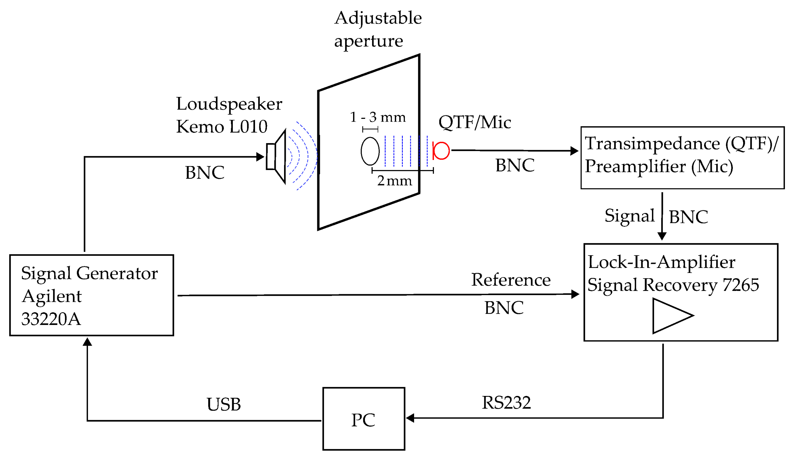
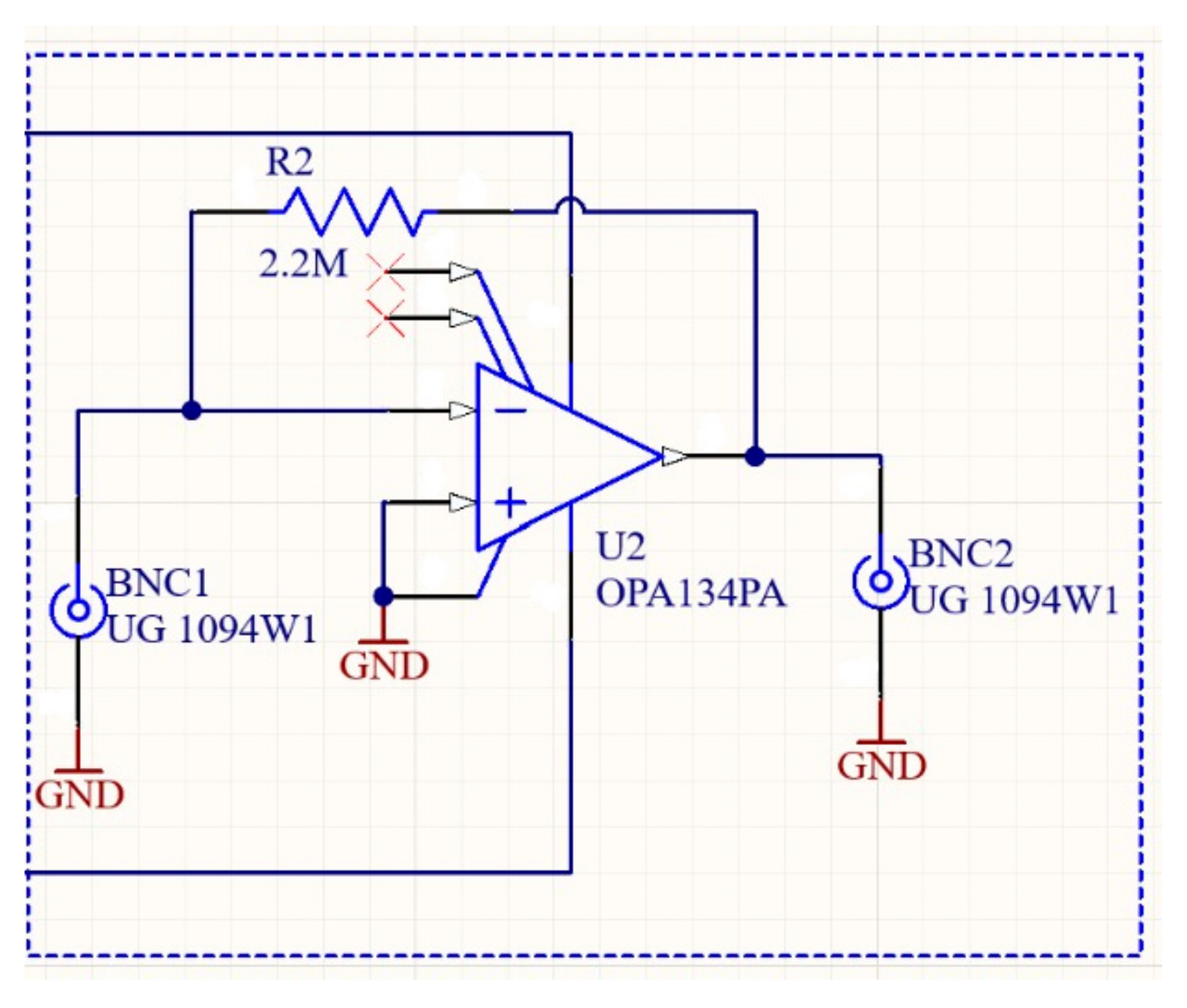
2.1. Experimental Setup

Figure 1 shows the experimental setup for the calibration of the QTF. The ultrasonic piezo loudspeaker L010 from Kemo Electronic GmbH (Geestland, Germany), with a membrane diameter of 41 mm, was used to generate an adjustable sound pressure wave. An aperture with an adjustable round opening in the center was placed in front of the loudspeaker to dampen the wave and to achieve a precise alignment in front of the sensors. The acoustic sensor (microphone or QTF, respectively) was placed at a distance of $\left(2.00\pm 0.05\right) \mathrm{mm}$, centrally, in front of the opening. The distance between the loudspeaker and the aperture was 3 cm, whereas the dimensions of the aperture plate were${\left(12\mathrm{cm}\right)}^2$.

The signal generator 33220A from Agilent (Santa Clara, CA, USA) produced the sinusoidal excitation voltage. Respective preamplifiers boosted the sound detector signals, while the Lock-In-Amplifier (LIA) Signal Recovery 7265 from AMETEK Scientific Instruments (Oak Ridge, TN, USA) recorded the signal at the excitation frequency with a time constant of 2 s. The entire experiment was controlled by a self-programmed MATLAB (9.14.0.2306882 (R2023a) Update 4) script on a PC.

The investigated QTF R38-32.768-12.5-EXT-5PPM from Raltron (Doral, FL, USA) had standard dimensions and a bandwidth of 4.72 Hz [14]. The electronic Q-factor of the QTF in a vacuum is 60,000, according to the manufacturer. Based on our own measurements, we have obtained an acoustic Q-factor of q = 6939 [14] in air. The QTF prongs each have a length of 6.00 mm, a width of 0.65 mm, a depth of 0.30 mm, and a gap of 0.20 mm (measured with microscope Stereo Discovery.V12 from Zeiss, Jena, Germany). The resonance frequency of the QTF of$f_R=\mathrm{32,758} \mathrm{H}\mathrm{z}$ deviates slightly from the above-mentioned standard frequency (within the manufacturing tolerances). When excited with sound, the oscillations of the QTF generate a small piezoelectric current. This current is converted into an output voltage using a homemade transimpedance amplifier with a feedback impedance of 2.2 MΩ. The electrical circuit of the QTF transimpedance amplifier is shown in Figure 2.

The operational amplifier (OPA) 134PA from Texas Instruments (Dallas, TX, USA) is the central component of the circuit. The typical electrical noise is specified by the manufacturer to be 0.00008% total harmonic distortion plus noise (THD+N). The resulting transimpedance for the circuit is $Z=-2.2\mathrm{kV}/\mathrm{mA}$. Its gain–bandwidth product (GBP) is 8 MHz, and the THD+N for 32 kHz is less than 0.001%. It is therefore reasonable to assume that the main source of noise is the tuning fork.

The calibration of the QTF was undertaken using a highly sensitive ultrasonic measuring microphone as a reference sensor. To do so, the QTF in Figure 1 was replaced with the 46BD 1/4″ CCP microphone set for pressure measurements from GRAS Acoustics (Holte, Denmark). It has a frequency range of 5 Hz to 70 kHz, a dynamic range of 44 dB (A) to 168 dB, and an average sensitivity of 1.45 mV/Pa. We operated it with the standard preamplifier 12AL 1-Channel CCP Power Module from GRAS Acoustics.

2.2. Methods

The main goal of this investigation is to relate the QTF signal to sound pressure. For this, it is essential to know the sound pressure at the location of the QTF. This measuring task is carried out with the above-mentioned microphone. The first step, therefore, is to determine the exact sensitivity of the microphone used at the resonance frequency of the QTF.

In the next step, the QTF signal as a function of pressure was measured. To do so, medium and high sound levels were generated with the ultrasonic loudspeaker in front of an aperture diameter of 1 mm (see Figure 1). The microphone and the QTF were placed (one after the other) at a 2.00 mm distance from the aperture. The lateral distance to the aperture was controlled using a high-precision vernier caliper from Mauser Inox (Isny, Germany), with an accuracy of $0.05\mathrm{mm}$. The microphone was positioned using an adjustable holder. The alignment was ensured by a marking on a mechanical guide. The sound wave hit the QTF approximately 2 mm below the tip, corresponding to approximately one-third of its total length, where the largest deflection is to be expected [15]. The microphone was placed with its most sensitive spot, the midpoint of its membrane, centered in front of the aperture opening. The setup was placed in a controlled environment with sound-absorbing walls to minimize external noise and environmental variability. The sensor signals were then recorded while the sound level was linearly increased. The measurements were averaged over several repetitions to ensure reliability and reduce random errors.

Subsequently, the background noise levels of the QTF and microphone were measured using the setup described in Figure 1. The signal of the QTF and the microphone were measured without a loudspeaker signal using their respective preamplifiers and the LIA. The random ambient noise levels were then compared in terms of distributed deviations.

In a final step, the acoustic detection limits of the microphone and the QTF were determined. To do so, the QTF sensitivity measurements were repeated at extremely low sound levels.

3. Results

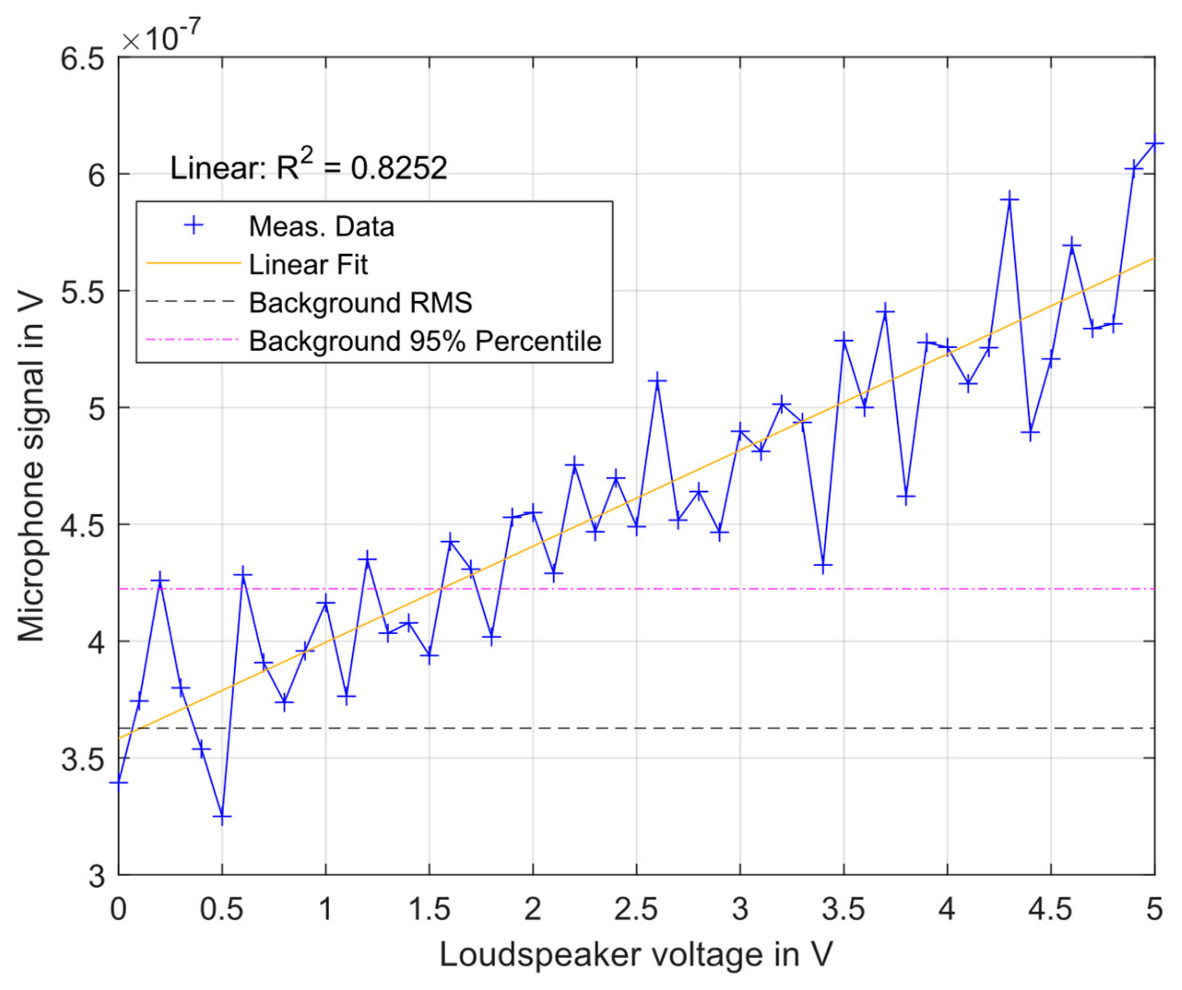
3.1. Microphone Sensitivity

For the QTF calibration, the sound pressure at its location must be measured with a reference detector. This has been accomplished using an extremely sensitive ultrasound-measuring microphone. The sound pressure was determined from its signal and its sensitivity, i.e., the proportionality constant between output voltage and sound pressure.

The microphone manufacturer provided a general sensitivity of the model series. However, for accurate results, the exact sensitivity of the microphone used is required. For this, the Multifunctional Sound Calibrator 42AG (Class 1) from GRAS Acoustics was used. This device mechanically generates a reference soundwave with a pressure amplitude of 1 Pascal ($L_C$ = 94 dB SPL) at a frequency of 1 kHz. The calibrator was put on the microphone head. Figure 3 shows the microphone signal as a function of time. The measured root-mean-square (RMS) was as follows: $V_0=1.0657·{10}^{-3}\mathrm{V}$. Accordingly, the sensitivity of $1.0657{\displaystyle \frac{\mathrm{m}\mathrm{V}}{Pa}}$ can be transferred into decibel levels using the following equation [16].

$$S_{Mic}\left(1\mathrm{kHz}\right)=20 ·{\log }_{10}\left({\displaystyle \frac{V_0}{2·{10}^{-5 }\mathrm{Pa} · {10}^{\frac{L_C}{20}}}} {\displaystyle \frac{\mathrm{Pa}}{\mathrm{V}}}\right) \mathrm{dB}$$

(1)

This leads to $S_{Mic}\left(1 \mathrm{kHz}\right)=-59.4679 \mathrm{d}\mathrm{B}.$

Figure 3. Microphone signal of calibrator at 1 kHz and 94 dB SPL.

Figure 3. Microphone signal of calibrator at 1 kHz and 94 dB SPL.

The manufacturer’s calibration certificate was used to adapt the 1 kHz sensitivity to the QTF resonance frequency:$f_R=\mathrm{32,758} \mathrm{H}\mathrm{z}$. Linear interpolation of the given values leads to a correction of $-0.2950 \mathrm{dB}$, resulting in a sensitivity of $S_{\mathrm{Mic}}\left(f_R\right)=-59.7629 \mathrm{dB}$, which corresponds to $1.0277{\displaystyle \frac{\mathrm{m}\mathrm{V}}{\mathrm{P}\mathrm{a}}}$.

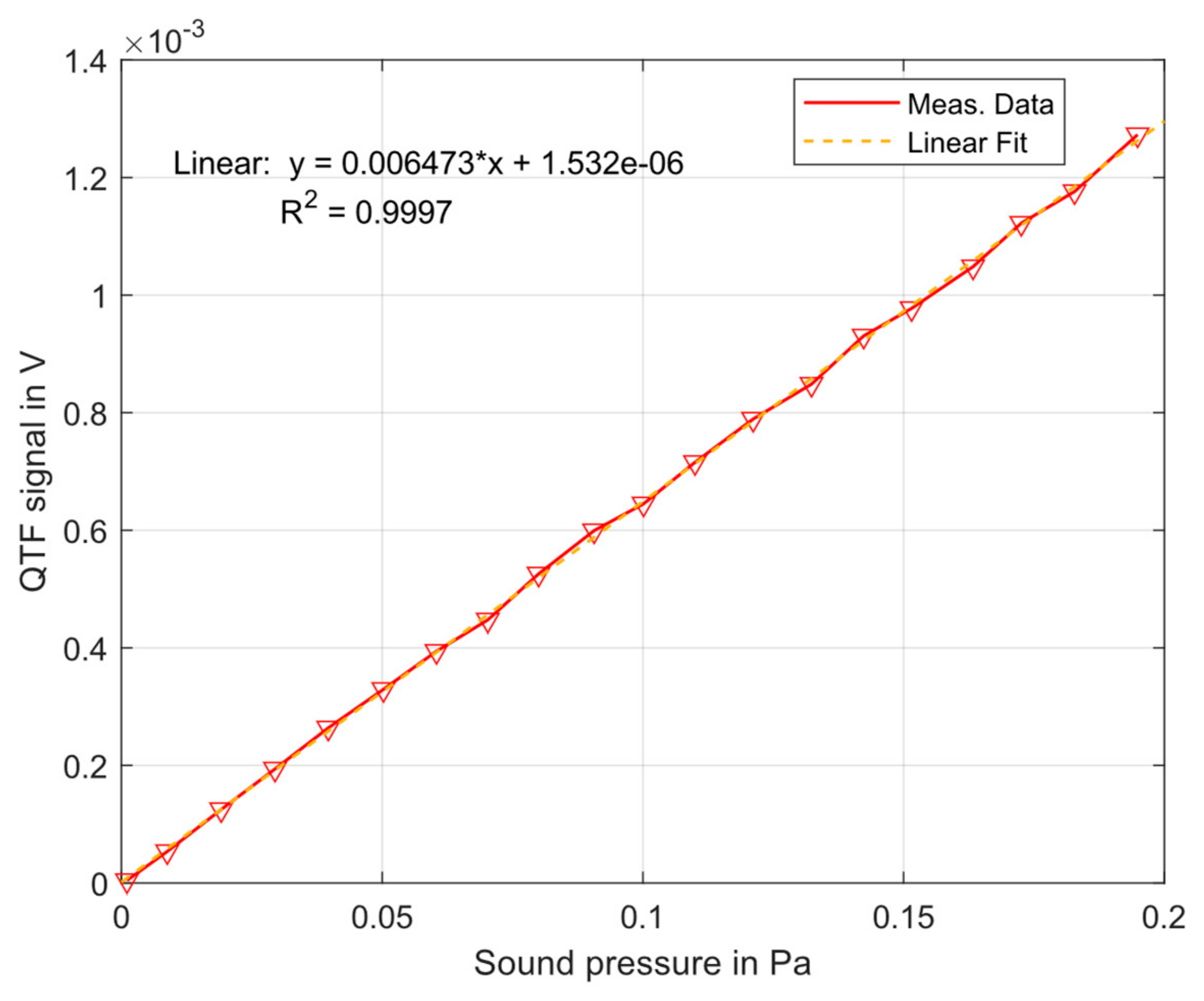
3.2. QTF Sensitivity

In the next step, we investigate whether the QTF signal is linearly dependent on the sound pressure; if this can be confirmed, a sensitivity will be determined.

Figure 4 shows the QTF output voltage as a function of medium and high sound pressure levels. Since the same measurements were carried out with a microphone of known sensitivity (see Section 3.1), the result can be presented in terms of sound pressure.

The coefficient of determination of the linear regression $R^2$ describes how well the model fits with the measured data. With $R^2=$ 99.97%, it is in excellent agreement. The sensitivity corresponds to the slope of the graph, which is $S_{\mathrm{QTF}}\left(f_R\right)=6.4730{\displaystyle \frac{\mathrm{mV}}{\mathrm{Pa}}}$. This corresponds to a level of $-43.78 \mathrm{dB}$. The QTF sensitivity is therefore a factor of 6.3 higher than that of the measuring microphone.

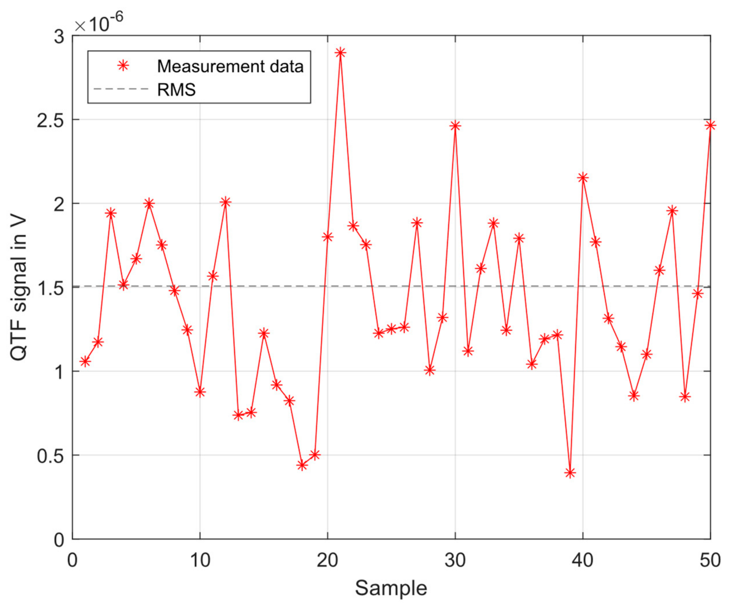
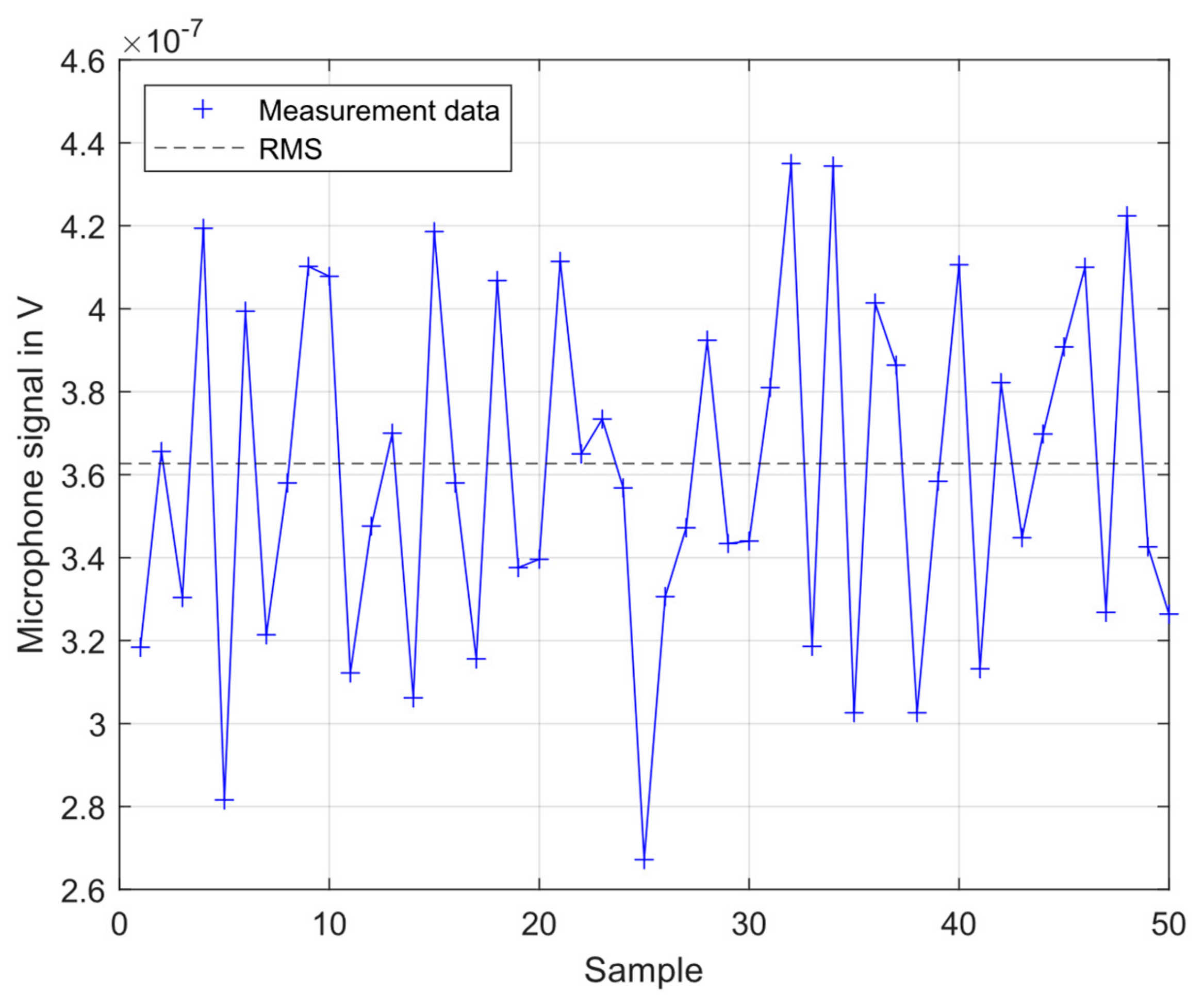
3.3. Microphone and Qtf Background Noise

The electrical and the ambient acoustic background signal interfere with the wanted signal. Their statistical fluctuation determines the detection limit of the sensors and should therefore be examined more closely. Figure 5 and Figure 6 show the background signals of the QTF and the microphone, respectively, as functions of time. The summed average deviation from the arithmetic mean $\epsilon$ is a measure of the background noise:

$$\epsilon ={\displaystyle \frac{\sum _{i=1}^n\left|x_i-\frac{1}{n}\sum _{i=1}^n{x}_i\right|}{\frac{1}{n}\sum _{i=1}^n{x}_i}},$$

(2)

with $n$ being the number of samples. One sample corresponds to 2 s averaging time.

For the QTF, $\epsilon$ is 15.15% of the mean value $1.51·{10}^{-6}$ V, whereas for the microphone, it is 4.86% of $3.63·{10}^{-7}$ V. The noise relative to the mean background signal is therefore lower for the microphone by a factor of approximately 3.

3.4. Microphone and QTF Detection Limit

The results of the background noise levels raise the question of whether the microphone exhibits a better detection limit than the tuning fork when acoustically stimulated at the QTF resonance frequency. Therefore, a sound signal, as low as possible, was generated with the loudspeaker behind the aperture and then successively increased.

Figure 7 and Figure 8 show the signal of the QTF and microphone, respectively, as functions of the sound pressure at the location of the sensors. Both graphs cover the range between 0.330 and 0.596 mPa. This corresponds to loudspeaker voltages between 0 and 5 V, whereas the signals at a loudspeaker voltage of 0 V are in accordance with the RMS of the background signals from the previous measurements. They are shown as dashed lines, while the 95% percentile of the noise are marked with dash-dotted lines.

The investigated sound pressure range corresponds to levels between 24 and 30 dBSPL, which is well below the specified limit for the microphone set with a preamplifier of 44 dB (A). However, with the help of the LIA, it was possible to clearly measure a linear signal increase with an increasing pressure level. For the QTF, ${R^2}_{\mathrm{QTF}}=92.89\mathrm{\%}$, while for the measuring microphone, ${R^2}_{\mathrm{Mic}}=82.49\mathrm{\%}$.

The signal-to-noise-ratio (SNR) in dB is defined as the difference between the signal level and the background noise, both in dB. For the QTF, the highest SNR, based on the linear fit in Figure 7, is 17.58 dB, whereas for the microphone in Figure 8, it is 3.84 dB. The same sound pressure level leads for the QTF, therefore, to a higher SNR compared to that of the microphone. Although the QTF has a larger standard deviation for repeated measurements at a single measurement point, it has a higher sensitivity and SNR for an acoustic signal at $f_R$.

The detection limits of the microphone and the QTF can be determined from their sensitivities,$S$, and the standard deviations of the background signal, $\sigma$.

$$x={\Phi }_{n,\alpha }·{\displaystyle \frac{\sigma }{S}}$$

(3)

The factor ${\Phi }_{n,\alpha }$ results from the significance level $\alpha$ and the number of the measured values $n$. For a significance level of $\alpha =0.5$ and four measurement repetitions, ${\Phi }_{n,\alpha }$ = 2.6 [17]. The standard deviation of the baseline measurement $\sigma$ corresponds to the mean standard deviation of the background signal from Section 3.3, and the sensitvities from Section 3.1 and Section 3.2, respectively, lead to the following detection limits for the microphone and the QTF:

$$\begin{gathered} x_{\mathrm{Mic}}=2.6·\left({\displaystyle \frac{3.3133·{10}^{-8} \mathrm{V}}{1.0277\frac{\mathrm{m}\mathrm{V}}{\mathrm{P}\mathrm{a}}}}\right)=8.3824·{10}^{-5} \mathrm{Pa} , \\ {x}_{\mathrm{QTF}}=2.6 ·\left({\displaystyle \frac{4.7386·{10}^{-7} \mathrm{V}}{6.4737\frac{\mathrm{m}\mathrm{V}}{\mathrm{P}\mathrm{a}}}}\right)=1.9031·{10}^{-4} \mathrm{Pa} . \end{gathered}$$

The detection limit of the microphone is lower than that of the QTF by approximately a factor of 2.

4. Discussion

The performance of the QTF as a sound detector was investigated and compared to a highly sensitive measuring microphone. The investigation revealed several distinct advantages and limitations for each sensing device.

Table 1. Key parameter for microphone and QTF in comparison.

Parameter	Unit	Microphone	QTF
Bandwidth	Hz	$5\dots 70,000 (\pm 2 \mathrm{dB}$)	4.72 (FWHM)
Dimension	mm	53 × 7 (incl. preamplifier)	6 × 3 (length × width)
Price (ca.)	Euro	2700	0.20
$\mathrm{Sensitivity} S\left(f_R\right)$	mV/Pa	$1.03$	$6.47$
$\mathrm{Linearity} \mathrm{of} \mathrm{resp}. R^2$ at low level	%	82.52	92.89
$\mathrm{Linearity} \mathrm{of} \mathrm{resp}. R^2$ at high level	%	100.00	99.97
$\mathrm{Background} \mathrm{noise} \epsilon$	% of RMS	4.86	15.15
$\mathrm{Detection} \mathrm{limit} x$	Pa	$8.38\times {10}^{-5}$	$1.90\times {10}^{-4}$
SNR at 0.596 mPa	dB	3.84	17.58

shows the results in direct comparison.

In summary, the microphone offers sound detection over an extremely wide frequency range. The QTF, on the other hand, is limited to its resonance frequency. A microphone is therefore recommended for all applications that require sound detection at multiple frequencies or over a frequency range. There are also MEMS microphones suitable for the ultrasonic range [18].

Within its resonance band, the QTF, however, is extremely sensitive to acoustic stimulation. It exhibits a higher SNR at a given sound pressure than the measuring microphone, although the QTF’s background noise relative to its RMS is higher than that of the microphone. However, since the QTF features a higher sensitivity, its linearity of response and detection limit is comparable with the microphone. This makes the QTF particularly suitable for detecting weak signals at its ultrasonic resonance frequency, which is interesting for applications such as PA spectroscopy or PA imaging [14]. The fact that the detection limit of the microphone is better than that of the QTF but the SNR is significantly lower seems contradictory. However, this is easily explained because the QTF shows a faster increase in SNR after reaching its detection limit

A particularly notable advantage of QTFs is their cost-efficiency. They are approximately four orders of magnitude less expensive than measuring microphones. Furthermore, their compact dimensions make them ideal for use in small setups. Both properties suggest the use of QTFs for applications aimed at mass production and cost optimization that tolerate the bandpass limitations.

Manufacturing tolerances causing slight variations in resonance frequency in QTFs can be easily addressed through simple calibration measurements enhancing the practicality of QTFs for targeted applications [19]. This variability is less impactful in tunable frequency systems but could limit fixed-frequency applications. To further enhance the performance of the QTF, the utilization of sophisticated amplifiers, exhibiting superior SNR characteristics in comparison to transimpedance amplifiers, can be employed [20,21].

In a standard substitution calibration, sensors of the same type are compared with one another. However, the QTF presents a unique challenge due to its different surface and vibration characteristics compared to the microphone. This discrepancy in excitation surfaces could result in the signal from the QTF rising to a higher relative extent than the signal from the microphone, even though the sound intensity is identical. This could be of additional benefit for applications with particularly low levels as it increases the SNR.

References

1. Lombardi, M.A. The evolution of time measurement, Part 2: Quartz clocks [Recalibration]. IEEE Instrum. Meas. Mag. 2011, 14, 41–48. [Google Scholar] [CrossRef]
2. Bloch, M.; Mancini, O.; McClelland, T. Performance of rubidium and quartz clocks in space. In Proceedings of the 2002 IEEE International Frequency Control Symposium and PDA Exhibition (Cat. No. 02CH37234), New Orleans, LA, USA, 31 May 2002; IEEE: Piscataway, NJ, USA, 2002. [Google Scholar]
3. Milde, T.; Hoppe, M.; Tatenguem, H.; Rohling, H.; Schmidtmann, S.; Honsberg, M.; Schade, W.; Sacher, J. QEPAS sensor in a butterfly package and its application. Appl. Opt. 2021, 60, C55–C59. [Google Scholar] [CrossRef] [PubMed]
4. De Carlo, M.; Menduni, G.; Sampaolo, A.; De Leonardis, F.; Spagnolo, V.; Passaro, V.M. Modeling and design of a semi-integrated QEPAS sensor. J. Light. Technol. 2020, 39, 646–653. [Google Scholar] [CrossRef]
5. Liberatore, N.; Viola, R.; Mengali, S.; Masini, L.; Zardi, F.; Elmi, I.; Zampolli, S. Compact GC-QEPAS for On-Site Analysis of Chemical Threats. Sensors 2022, 23, 270. [Google Scholar] [CrossRef] [PubMed]
6. Li, B.; Menduni, G.; Giglio, M.; Patimisco, P.; Sampaolo, A.; Zifarelli, A.; Wu, H.; Wei, T.; Spagnolo, V.; Dong, L. Quartz-enhanced photoacoustic spectroscopy (QEPAS) and Beat Frequency-QEPAS techniques for air pollutants detection: A comparison in terms of sensitivity and acquisition time. Photoacoustics 2023, 31, 100479. [Google Scholar] [CrossRef] [PubMed]
7. Liu, Y.; Lin, H.; Montano, B.A.Z.; Zhu, W.; Zhong, Y.; Kan, R.; Yuan, B.; Yu, J.; Shao, M.; Zheng, H. Integrated near-infrared QEPAS sensor based on a 28 kHz quartz tuning fork for online monitoring of CO2 in the greenhouse. Photoacoustics 2022, 25, 100332. [Google Scholar] [PubMed]
8. Angstenberger, S.; Floess, M.; Schmid, L.; Ruchka, P.; Steinle, T.; Giessen, H. Coherent control in quartz-enhanced photoacoustics: Fingerprinting a trace gas at ppm-level within seconds. Optica 2025, 12, 1–4. [Google Scholar]
9. Yang, M.; Wang, Z.; Sun, H.; Hu, M.; Yeung, P.T.; Nie, Q.; Liu, S.; Akikusa, N.; Ren, W. Highly sensitive QEPAS sensor for sub-ppb N2O detection using a compact butterfly-packaged quantum cascade laser. Appl. Phys. B Laser Opt. 2024, 130, 6. [Google Scholar] [CrossRef]
10. Liang, T.; Qiao, S.; Chen, Y.; He, Y.; Ma, Y. High-sensitivity methane detection based on QEPAS and H-QEPAS technologies combined with a self-designed 8.7 kHz quartz tuning fork. Photoacoustics 2024, 36, 100592. [Google Scholar] [CrossRef] [PubMed]
11. Sampaolo, A.; Menduni, G.; Patimisco, P.; Giglio, M.; Passaro, V.M.; Dong, L.; Wu, H.; Tittel, F.K.; Spagnolo, V. Quartz-enhanced photoacoustic spectroscopy for hydrocarbon trace gas detection and petroleum exploration. Fuel 2020, 277, 118118. [Google Scholar] [CrossRef]
12. Hussain, D.; Zhang, H.; Song, J.; Yongbing, W.; Meng, X.; Xinjian, F.; Xie, H. Amplitude calibration of quartz tuning fork (QTF) force sensor with an atomic force microscope. In Proceedings of the 2017 IEEE 17th International Conference on Nanotechnology (IEEE-NANO), Pittsburgh, PA, USA, 25–28 July 2017; IEEE: Piscataway, NJ, USA, 2017. [Google Scholar]
13. Dedeoglu, A.; Karadas, N.; Unal, M.A.; Kocum, I.C.; Serdaroglu, D.C.; Ozkan, S.A. Calibration of Quartz Tuning Fork transducer by coulometry for mass sensitive sensor studies. J. Electroanal. Chem. 2019, 834, 8–16. [Google Scholar]
14. Falkhofen, J.; Bahr, M.-S.; Baumann, B.; Wolff, M. Quartz enhanced photoacoustic spectroscopy on solid samples. Sensors 2024, 24, 4085. [Google Scholar] [CrossRef] [PubMed]
15. Patimisco, P.; Sampaolo, A.; Zheng, H.; Dong, L.; Tittel, F.K.; Spagnolo, V. Quartz–enhanced photoacoustic spectrophones exploiting custom tuning forks: A review. Adv. Phys. X 2017, 2, 169–187. [Google Scholar]
16. GRAS Sound & Vibration. In Instruction Manual 42AG Multifunction Calibrator; GRAS Sound & Vibration: Holte, Denmark, 2017; Available online: google.com/url?sa=t&rct=j&q=&esrc=s&source=web&cd=&ved=2ahUKEwigmbLvlqWMAxW2cfEDHedhJFQQFnoECBsQAQ&url=https%3A%2F%2Fwww.grasacoustics.com%2Ffileadmin-gras%2FProducts%2FFiles%2Fmanual_42AG_LI0196.pdf&usg=AOvVaw2zSv6vyAbbX1oodBTclSgp&opi=89978449 (accessed on 5 February 2025).
17. DIN 32645; Chemische Analytik–Nachweis-, Erfassungs-und Bestimmungsgrenze unter Wiederholbedingungen, Verfahren, Auswertung. DIN Media: Berlin, Germany, 2008.
18. Falkhofen, J.; Wolff, M. Near-ultrasonic transfer function and SNR of differential MEMS microphones suitable for photoacoustics. Sensors 2023, 23, 2774. [Google Scholar] [CrossRef] [PubMed]
19. Wu, H.; Dong, L.; Zheng, H.; Yu, Y.; Ma, W.; Zhang, L.; Yin, W.; Xiao, L.; Jia, S.; Tittel, F.K. Beat frequency quartz-enhanced photoacoustic spectroscopy for fast and calibration-free continuous trace-gas monitoring. Nat. Commun. Nat. Commun. 2017, 8, 15331. [Google Scholar] [CrossRef] [PubMed]
20. Winkowski, M.; Stacewicz, T. Low noise, open-source QEPAS system with instrumentation amplifier. Sci. Rep. 2019, 9, 1838. [Google Scholar]
21. Wieczorek, P.Z.; Starecki, T.; Tittel, F.K. Improving the signal to noise ratio of QTF preamplifiers dedicated for QEPAS applications. Appl. Sci. 2020, 10, 4105. [Google Scholar] [CrossRef]
Figure 1. Measurement setup.
Applsci 15 03655 g001
Figure 2. Electrical circuit of the homemade QTF transimpedance amplifier.
Applsci 15 03655 g002
Figure 4. QTF signal as function of sound pressure (medium/high levels).
Applsci 15 03655 g004
Figure 5. QTF background signal.
Applsci 15 03655 g005
Figure 6. Microphone background signal.
Applsci 15 03655 g006
Figure 7. QTF signal as a function of sound pressure (low levels).
Applsci 15 03655 g007
Figure 8. Microphone signal as a function of sound pressure (low levels).
Applsci 15 03655 g008