Abstract
Hypergraph analysis extends traditional graph theory by enabling the study of complex, many-to-many relationships in networks, offering powerful tools for understanding brain connectivity. This case study introduces a novel methodology for constructing both graphs and hypergraphs of functional brain connectivity during figurative attention tasks, where subjects interpret the ambiguous Necker cube illusion. Using a frequency-tagging approach, we simultaneously modulated two cube faces at distinct frequencies while recording electroencephalography (EEG) responses. Brain connectivity networks were constructed using multiple measures—coherence, cross-correlation, and mutual information—providing complementary insights into functional relationships between regions. Our hypergraph analysis revealed distinct connectivity patterns associated with attending to different cube orientations, including previously unobserved higher-order relationships between brain regions. The results demonstrate bilateral cortico–cortical interactions and suggest integrated processing hubs that may coordinate visual attention networks. This methodological framework not only advances our understanding of the neural basis of visual attention but also offers potential applications in attention monitoring and clinical assessment of attention disorders. While based on a single subject, this proof-of-concept study establishes a foundation for larger-scale investigations of brain network dynamics during ambiguous visual processing.
1. Introduction
Understanding brain connectivity in response to external stimuli is essential for uncovering the mechanisms behind information processing, perception, attention, and decision-making. Functional connectivity, which identifies active brain regions exhibiting correlated frequency, phase, and amplitude, can be analyzed in both frequency and time domains [1]. When a sufficiently large population of neurons synchronizes, their collective electrical activity becomes detectable through brain imaging techniques such as electroencephalography (EEG). To examine the emergence and dynamic evolution of functional brain networks, researchers often apply complex network theory, grounded in mathematical graph theory [2,3]. By representing brain regions as nodes and their interactions as links, this approach has facilitated the study of biorhythmic connections across different brain areas [4,5]. It has also proven valuable in identifying individual cognitive differences [6], diagnosing neurological disorders [7,8,9], and assessing aging-related neural changes [10,11,12,13].
EEG-based functional connectivity networks have become essential tools for understanding individual variability in brain activation patterns during cognitive tasks [14,15]. These networks provide valuable insights into how different brain regions interact, shedding light on the neural mechanisms underlying attention and other cognitive processes. Traditional graph-theoretic approaches model functional connectivity by representing brain regions as vertices and their functional interactions as edges [4]. However, these methods primarily capture second-order relationships—interactions between pairs of brain regions—while neglecting higher-order relationships that are fundamental to complex neural processing.
Since cognitive processes such as attention involve dynamic and multifaceted interactions across multiple brain regions, conventional functional connectivity networks fail to provide a complete picture by only capturing pairwise relationships. To overcome this limitation, hypergraph-based connectivity models have been introduced. Unlike traditional graphs, hypergraphs allow for the representation of multi-node interactions through hyperedges, enabling a richer and more comprehensive characterization of brain connectivity.
Hypergraphs have recently gained prominence as an advanced framework for investigating brain connectivity [16,17,18,19,20,21,22,23,24,25,26,27,28,29,30]. Unlike conventional graphs that are limited to pairwise relationships, hypergraphs extend graph theory to model complex, multi-region interactions simultaneously [31,32]. This approach offers a more nuanced and holistic view of functional brain networks by capturing the intricate, dynamic interactions among multiple neural regions. Through hypergraph analysis, researchers can gain deeper insights into how brain regions integrate, synchronize, and adapt to support cognitive functions, providing novel perspectives on neural organization and functionality.
Hypergraphs representing brain connectivity have been constructed using neurophysiological data from various imaging modalities. Most studies have focused on functional magnetic resonance imaging (fMRI) data, particularly in the resting state [16,17,18,19,20,21,22,23,24]. Structural MRI has also been employed for hypergraph-based connectivity modeling [25]. Additionally, researchers have developed hypergraphs using multimodal data that integrate MRI with fluorodeoxyglucose positron emission tomography (PET) and cerebrospinal fluid analysis [29]. Beyond MRI-based studies, both invasive intracranial EEG [26] and noninvasive EEG [27,28] have been used to construct hypergraphs. Magnetoencephalography (MEG) data have also been explored in hypergraph-based connectivity studies [30].
The versatility of hypergraph-based connectivity modeling has led to applications in diverse areas, including emotion recognition [22,27], motor imagery [28], and the diagnosis of neurological disorders such as mild cognitive impairment [18,21,29], schizophrenia [20], autism spectrum disorder [24], Alzheimer’s disease [25,29], and epileptic seizure detection [26]. Many of these studies employ correlation-based metrics to measure functional connectivity, with Pearson correlation being a widely used approach for quantifying neural interactions [33]. Given the importance of attentional processes in cognitive health, hypergraph-based connectivity models offer a promising avenue for understanding the neural mechanisms underlying attention and related cognitive functions.
Attention is a crucial cognitive function, and its impairment is associated with various neurological and psychiatric disorders, including cognitive decline, dementia, attention deficit hyperactivity disorder, and autism spectrum disorder. These conditions affect a broad range of cognitive and behavioral abilities, such as learning, problem-solving, communication, and social interaction. Individuals with attention deficits may struggle to express their experiences or understand others’ perspectives, which can hinder their development of essential social and learning skills. Electroencephalography (EEG) is a widely used modality for assessing attention. While many studies have focused on the relationship between P-300 event-related potentials and attention in EEG signals, others have explored spectral analysis as an alternative approach [34,35,36,37,38]. The use of hypergraphs to model brain connectivity could provide deeper insights into the neural mechanisms underlying attention deficits by capturing the complex, multi-dimensional relationships within brain networks. This approach may complement traditional EEG-based methods, offering a more comprehensive understanding of attention-related impairments and their neural correlates.
This study is motivated by the growing interest in machine learning techniques for the early diagnosis and prediction of neurodegenerative diseases based on hypergraphs of brain connectivity. The primary objective of this study is to develop a method for constructing hypergraphs of brain connectivity to enhance our understanding of brain functionality during figurative attention. Unlike traditional pairwise graphs, hypergraphs provide a more comprehensive representation by capturing the most significant connections and disconnections across multiple brain lobes, identified through different connectivity measures such as coherence, correlation, and mutual information. To investigate this, we use the Necker cube—an ambiguous figure requiring attentional focus for orientation interpretation (left- or right-facing). EEG data is recorded while the participant performs three cognitive tasks: (i) passive viewing without interpreting the cube’s orientation (MI), (ii) imagining the cube as left-oriented (MLV), and (iii) imagining it as right-oriented (MRV). Task (i) serves as a baseline for involuntary attention, whereas tasks (ii) and (iii) assess voluntary attention. By comparing brain connectivity patterns across these conditions, we aim to identify changes in connectivity associated with voluntary and involuntary attention. These insights contribute to understanding how figurative attention influences brain network dynamics, particularly in sustaining focus on a specific perceptual interpretation.
A graphical framework of our study is presented in Figure 1.

Figure 1.
Main steps for constructing hypergraphs of brain connectivity during figurative attention. EEG data are recorded while the subject performs three cognitive tasks: MI, MLV, and MRV. Based on three connectivity measures (coherence, correlation, and mutual information), corresponding pairwise graphs are constructed. A sparsification procedure is then applied to generate hypergraphs that capture higher-order interactions associated with attention to the left-oriented and right-oriented cube.
To the best of our knowledge, this work presents the first hypergraph-based analysis of functional brain connectivity associated with attention. We demonstrate how hypergraphs can be constructed to represent brain connectivity patterns associated with attention, which may, in the future, contribute to the diagnosis and prediction of attention-related disorders. Using EEG data from a subject exhibiting strong attentional engagement, we construct both pairwise graphs and hypergraphs based on three important connectivity measures—coherence [39], cross-correlation [40], and mutual information [41]. Our analysis investigates how functional connectivity differs when the subject actively focuses on one interpretation of the Necker cube’s orientation compared to a neutral attentional state.
The remainder of this paper is organized as follows: Section 2 introduces the mathematical foundations underlying our methods. Section 3 details the experimental paradigm and methodology. Section 4 describes the procedures for analyzing the experimental EEG data. Section 5 and Section 6 present results on the construction of attention-based pairwise graphs and hypergraphs, respectively. Section 7 provides an in-depth discussion of our findings, followed by key conclusions in Section 8. Additional details on graph construction are included in the Appendices.
2. Mathematical Basis
In this section, we provide the most important definitions of pairwise graphs and hypergraphs, as well as the measures of brain connectivity that we utilize in this study: coherence, cross-correlation, and mutual information.
2.1. Main Definitions
A plain graph G is an abstract mathematical structure composed of a finite set of n vertices (or nodes) V and a set of m edges (or links) E, where each edge represents an interaction between a pair of vertices. Mathematically, the plain graph is defined as
The plain graph is commonly represented by its adjacency matrix A, which can be either binary (indicating the presence or absence of a connection between two vertices) or numerical (reflecting the strengths or weights of the connections between edges). A graph with labels assigned to its edges and vertices is referred to as a labeled graph. A label of edge j is its weight (or connectivity measure), i.e., , while a label of vertex i is the sum of weights of all edges which connect this vertex with other nodes, i.e.,
where is the indicator function, equal to weight of edge j if this edge is incident to vertex i, and 0 otherwise.
In contrast to a plain graph, where an edge connects only two vertices, a hypergraph generalizes this concept by allowing a single edge, called a hyperedge, to connect more than two vertices [31,32]. Formally, a hyperedge is defined as a collection of links that connect two or more edges with significantly correlated temporal or spectral profiles. Thus, a hypergraph is defined by a set of such hyperedges and nodes, offering a powerful framework for modeling and analyzing complex relationships, particularly in systems such as brain networks.
To illustrate this, consider a brain neural network that is conventionally partitioned into n distinct regions, referred to as nodes or vertices. Signals from these regions can be recorded using various neuroimaging modalities, such as EEG, MEG, or fMRI. When the brain is exposed to a stimulus, neuronal activity in specific regions associated with the stimulus is either activated or deactivated, and information about this process is encoded in the corresponding vertices. By capturing the relationships between these regions, a hypergraph is defined by a set of n vertices and a set of m hyperedges as
where each hyperedge represents a specific measure of connectivity. In this work, we consider widely used measures of brain connectivity, such as coherence, cross-correlation, and mutual information. These measures can be computed for specific spectral bands and time intervals of interest, allowing for a detailed characterization of functional relationships within the brain.
A hypergraph is characterized by its order and size. The order refers to the number of vertices , while the size corresponds to the number of hyperedges . Furthermore, both vertices and hyperedges are associated with a degree (Deg), which quantifies their connectivity within the hypergraph. Specifically, the degree of a vertex is defined as the number of hyperedges incident to it, whereas the degree of a hyperedge is defined as the number of vertices incident to it. Mathematically, these degrees can be expressed as follows:
where is the indicator function, equal to 1 if the condition is satisfied and 0 otherwise. These degree measures provide insights into the topological structure of the hypergraph, highlighting the centrality of vertices and the complexity of hyperedges in capturing higher-order interactions.
If a vertex v is covered by two or more hyperedges, we say that these hyperedges are adjacent through v (). Similarly, the vertices covered by a hyperedge e are considered adjacent through e ().
A hypergraph can be represented in several equivalent forms, including an incidence graph, an incidence matrix , and a hyperedge weight matrix .
An incidence graph (also known as a bipartite graph representation) is a way to represent a hypergraph by transforming it into a standard graph. In this representation, the hypergraph’s vertices and hyperedges are treated as two distinct sets of nodes in a bipartite graph.
The incidence matrix is defined as
where represents the i-th vertex and represents the j-th hyperedge. This matrix captures the membership of vertices in hyperedges, providing a binary representation of the hypergraph structure.
A hyperedge weight matrix encodes the significance of each hyperedge in the hypergraph. Specifically, the weight of each hyperedge is located at the corresponding diagonal entry of , such that
where represents the weight of the j-th hyperedge. In this work, the weight is defined as the degree of the hyperedge , i.e., Deg. This weighting scheme reflects the topological importance of each hyperedge within the hypergraph.
A hypergraph can be modified by transforming vertices into edges () and vice versa. This transformation is called “duality of hypergraphs” and is denoted as , where , with representing the set of all edges incident to vertex . The degree of vertices in a dual hypergraph is equal to the degree of hyperedges in , while the degree of the hyperedges remains unchanged from . This relationship can be expressed as follows:
Several hypergraphs can be represented as multilayer hypergraphs, which generalize both hypergraphs and multilayer networks to model complex relationships in multi-dimensional or multi-modal data. This framework extends traditional hypergraphs by incorporating multiple layers, where each layer represents a distinct context, domain, or interaction type among entities.
A multilayer hypergraph is formally defined as follows:
where is the set of layers. Each layer represents a different context, interaction type, or domain. Each layer represents a different context or interaction type, and hyperedges can be associated with one or more layers, enabling the representation of complex, heterogeneous relationships beyond simple pairwise connections.
Key properties of multilayer hypergraphs include the following: (i) cross-layer connectivity—nodes can belong to multiple layers, allowing hyperedges to span across different layers, (ii) layer-specific interactions—each layer captures a distinct type of interaction, such as coherence, correlation, or mutual information, and (iii) heterogeneous hyperedges—hyperedges can vary in size and exist across multiple layers, enabling flexible modeling of higher-order relationships. By leveraging these properties, multilayer hypergraphs provide a powerful framework for analyzing brain connectivity across different cognitive states or regions.
Another common approach to representing higher-order relationships is the clique expansion of a hypergraph. In this transformation, each hyperedge is replaced by a clique—a complete subgraph—connecting all vertices within that hyperedge. This method is widely used to approximate hypergraphs with graphs. The clique expansion algorithm constructs a graph from the original hypergraph by replacing each hyperedge with edges between every pair of its vertices [42]. Thus, the vertices in a hyperedge e form a clique in . In the weighted clique expansion, each edge within the clique corresponding to hyperedge e is assigned a weight , reflecting the discriminative model used in the transformation.
2.2. Summarization
Graphs of real datasets are often very massive. For example, the graph constructed on the basis of the MEG data has 306 nodes, each representing time series recorded by magnetic sensors [30,43]. The manipulation of such large networks requires high computational capacity and extensive time. To decrease the communicational cost, a graph summarization technique is used [44]. Summarization methods allow one to reduce the graph size by extracting the most important information from the original graph. Then, the resultant summary graph can be queried, analyzed, and understood more efficiently using existing tools and algorithms. The resultant graph can more easily visualize the dataset that is originally too large to load into memory. In addition, real graph data are frequently large scale and considerably noisy, with many hidden, unobserved, or erroneous links and labels. Such noise hinders analysis by increasing the workload of data processing and hiding the more important information. Summarization serves to filter out noise and reveal specific features in the data.
Summarization is application-dependent and can be made using various methods. The most popular summarization techniques are node grouping and edge grouping. While the node-grouping methods recursively aggregate nodes into “supernodes” based on an application-dependent optimization function, which can be based on structure and/or attributes, e.g., clustering techniques and map each densely connected cluster to a supernode, edge-grouping methods aggregate edges into hyperedges. In this paper, we apply the latter approach that compresses neighborhoods around high-degree nodes, accelerating query processing and enabling direct operations on the compressed graph. The edge-grouping method was used by Maccioni and Abadi [45], who introduced “compressor nodes”, which represent common connections of high-degree nodes. They assumed that high-degree nodes are surrounded by redundant information that can be synthesized and eliminated. To provide global guarantees and reduce the scope of compressor handling during query processing, dedensification only occurs when every node has at most one outgoing edge to a compressor node, and every high-degree node has incoming edges coming only from a compressor node. These guarantees are then used to create query processing algorithms that enable direct pattern matching queries on the compressed graph.
Other summarization techniques imply simplification or sparsification. These methods streamline an input graph by removing less “important” nodes or edges, resulting in a sparsified graph. In the brain connectivity network, some edges are more indicative of predicting cognitive performance. Therefore, the node grouping layer is designed to “hide” the non-indicative (‘noisy’) edges by grouping them into a cluster (supernode), thus highlighting the indicative edges. Finally, there are influence-based approaches that aim to discover a high-level description of the influence propagation in large-scale graphs. Techniques in this category formulate the summarization problem as an optimization process in which some quantity related to information influence is maintained.
The output of a summarization procedure can take one of two forms: (i) a sparsified graph, which retains only a subset of nodes and/or edges from the original graph, or (ii) a hypergraph composed of selected nodes united by hyperedges. Unlike traditional graphs, hypergraphs allow nodes to belong to multiple hyperedges, enabling the representation of complex, higher-order relationships within the data. In this paper, we integrate both approaches, leveraging sparsified graphs as a foundation to construct hypergraphs that model brain connectivity associated with attention. This combined methodology enables the capture of intricate neural interactions while maintaining computational efficiency, providing a robust framework for analyzing attention-related brain networks.
2.3. Coherence
One of the key measures to quantify neuronal synchrony is event-related coherence [39,46,47]. It examines the frequency-domain relationship between two signals, reflecting the extent to which their spectral components are synchronized. Specifically, it assesses the consistency of the relative amplitude and phase between two signals within a given frequency range. Mathematically, it is a linear method that generates a symmetrical matrix, which lacks directional information. When two signals are identical, the coherence value is 1, whereas it approaches 0 as the signals become increasingly dissimilar. Since its introduction, coherence has been widely employed in brain connectivity studies involving both patients and healthy individuals. These studies span a diverse range of applications, including working memory [48], brain lesions [49], hemiparesis [50], resting-state networks [51], schizophrenia [52,53], responses to panic medications [54], and motor imagery [55]. Due to the inherent variability in human brains, distinct patterns of coherent neuronal activity have been observed across individuals. For instance, when exposed to flickering visual stimuli, subjects exhibit coherent responses in the visual cortex at the flicker frequency and its harmonics, with varying sizes of coherent neural networks [43,56].
Coherence between two signals ( and ) is defined as
where and are the auto spectral densities of and signals, respectively, and is the cross-spectral density. The coherence function estimates the extent to which may be predicted from by an optimum linear least squares function.
Coherence values always satisfy . In our study, since we focus on the changes in coherence induced by attention (), these differences can be either positive or negative, thus satisfying . In the subsequent analysis, we will refer to an increase in coherence () as coherence and a decrease in coherence () as anticoherence. This distinction allows us to better characterize the dynamic shifts in neural connectivity associated with attentional processes.
2.4. Cross-Correlation
Unlike previous studies that rely on Pearson correlation for constructing functional connectivity networks [57,58], our approach employs cross-correlation analysis. The Pearson correlation has several limitations, including sensitivity to delays in neural responses and potential confounding effects from other brain regions. To address these issues, we used cross-correlation analysis, selecting the optimal time delay at which correlation is maximized.
Cross-correlation measures the similarity between two time series as a function of the time lag between them. This method provides a robust and sensitive approach for analyzing EEG signals recorded simultaneously from different channels, independent of their amplitudes [40]. By accounting for time lags, cross-correlation allows for the evaluation of relationships between signals not only at the same moment but also at different time points, offering deeper insights into temporal dependencies and synchronization patterns in neural activity.
The normalized cross-correlation between two EEG channels and , at a given time lag , is calculated as follows:
where and demote the mean values of and , respectively. For each pair of channels, we identify the time lag at which attains its maximum value and use this peak correlation value in our subsequent analysis. This approach ensures that we capture the strongest temporal relationship between the signals, providing a robust basis for reconstructing a functional connectivity network.
Cross-correlation values range from and 1. To analyze changes in cross-correlation induced by attention, we define the difference in cross-correlation (), which can take values between and 2. For clarity, we refer to cases where as correlation and cases where as anticorrelation. This distinction helps characterize neural connections that emerge (increased synchrony) and disappear (decreased synchrony) due to attention.
2.5. Mutual Information
Since its introduction by Shannon [59], mutual information has been used across various fields to quantify coupling or information transmission between systems [60]. In neuroscience, several studies have employed mutual information analysis to investigate information transfer in the brain. For example, Jeong et al. [41] applied this method to multi-channel EEG data to assess information flow between cortical regions in Alzheimer’s disease (AD) patients.
Cross mutual information (CMI) measures the information gained about one system from observing another, in contrast to auto mutual information, which quantifies mutual information between two parts of he same time series separated by a lag . Unlike traditional correlation functions, which capture only linear dependencies, CMI detects both linear and nonlinear statistical relationships between time series. CMI between measurement from system X and from system Y represents the amount of information provides about . Thus, CMI serves as a measure of dynamical coupling or information transmission between X and Y. When applied to EEG data, it can be interpreted as an indicator of functional connectivity between brain regions. If two systems are entirely independent, their CMI is zero, meaning no information is transmitted between them. Therefore, in our case, CMI quantifies the information flow between different brain areas.
CMI is calculated as
where and are the normalized histograms of the distributions of measurements x and y, respectively, and denotes their joint probability density.
In this study, we compute the time-delayed CMI, , which quantifies mutual information between EEG signals from each pair of channels as a function of a time delay. To assess information transmission between different cortical areas, we select the peak CMI value within a time delay range of ms for each electrode pair.
CMI measures the degree of dependence between X and Y, ranging from 0 to entropy H of X. A value of indicates mutual independence, whereas signifies that one signal completely determines the other. Similar to coherence and correlation measures, changes in CMI due to attention () can be either positive or negative. Specifically, positive values () indicate information gain, while negative values () correspond to information loss.
3. Materials and Experimental Methods
3.1. Participant
In this case study, we analyze the EEG data of a healthy 22-year-old female subject, recorded during experiments using a flickering image paradigm. This study was conducted at the Center for Biomedical Technology, Universidad Politécnica de Madrid, Spain. This subject was selected from a pool of 28 subject participants as the one demonstrating the highest level of attention (subject #2 from [38]). Before the experiment began, the subject provided written informed consent, ensuring anonymized data processing and compliance with data protection regulations. The subject was also briefed on the experiment’s objectives and duration. The EEG study followed the ethical guidelines of the Declaration of Helsinki and was approved by the Ethics Committee of the Universidad Politécnica de Madrid (Ethics Approval Code: 2020-096) prior to participant recruitment.
3.2. Stimulus
The subject was presented with a visual stimulus—the Necker cube—displayed as a white line drawing on a black screen. The image, approximately cm in size, was shown on a 22-inch liquid crystal monitor with a refresh rate of 60 Hz and luminance of 100 cd/m2. The Necker cube was chosen for its ambiguous nature, allowing for perceptual alternation between left and right orientations.
The cube’s pixel brightness alternated between black (0 in an 8-bit format) and gray (200) following a square-wave modulation. This modulation was applied at frequencies Hz and Hz to the left and right faces of the cube, respectively, consistent with previous studies [43,56]. These modulation frequencies generated frequency tags in the fast Fourier transform (FFT) spectra of the EEG signal, particularly in spectral regions around and within the visual cortex. To present the visual stimuli, we developed custom software using the PsychoPy 2024.2.5 and Python 3.12.4 platforms.
3.3. Experimental Setup
The EEG recording setup consisted of a 16-channel LIVEAMP amplifier, a standard wireless 16-channel cap, a reference channel, and a ground channel. The cap was fitted with slim active electrodes from EASYCAP GmbH (Wörthsee, Germany). To enhance conductivity, a conductive gel was applied to each electrode.
The experiments took place in a dimly lit room, with the subject seated comfortably in front of a computer monitor positioned 80 cm away. The visual stimulus subtended an approximate viewing angle of 8 degrees.
The EEG signal was recorded using BrainVision Recorder (version 1.27) from Brain Products GmbH, a highly reliable software for EEG signal acquisition. One of its key features is real-time impedance monitoring, which ensures optimal electrode-to-scalp contact by detecting potential faulty connections and maintaining impedance below the predefined threshold of <10 k. EEG data were sampled at a rate of 500 Hz.
The data acquisition details can be found in Appendix A.
3.4. Experimental Paradigm
The experiment comprised a series of Necker cube presentations, each lasting approximately 30 s, with 20 s intervals between presentations. During these intervals, the subject was allowed to blink. EEG recordings were continuously conducted throughout cube observation to monitor brain activity in real time.
Before the main experiment, the participant underwent a training session using a non-flickering Necker cube to familiarize herself with distinguishing between left- and right-oriented perceptions. The subject was instructed to complete three tasks: (1) observing the first cube image without interpreting its orientation, (2) perceiving the second cube image as left-oriented, and (3) perceiving the third cube image as right-oriented.
In the main experiment, the subject performed similar tasks but with a flickering (modulated) Necker cube. The first task involved passive observation of the cube without interpretation of its orientation (MI: modulated involuntary). In the second task (MLV: modulated left voluntary) and third task (MRV: modulated right voluntary), the subject was instructed to voluntarily perceive the cube as left- or right-oriented, respectively.
Figure 2 illustrates how the subject perceives the left and right cube orientations. The way the cubes are perceived depends on the task (MLV or MRV). Figurative attention to a specific cube orientation leads to the activation and deactivation of different neural pathways. The passive viewing condition (MI) is not included because the brain’s perception is unstable, alternating between left- and right-cube orientations.
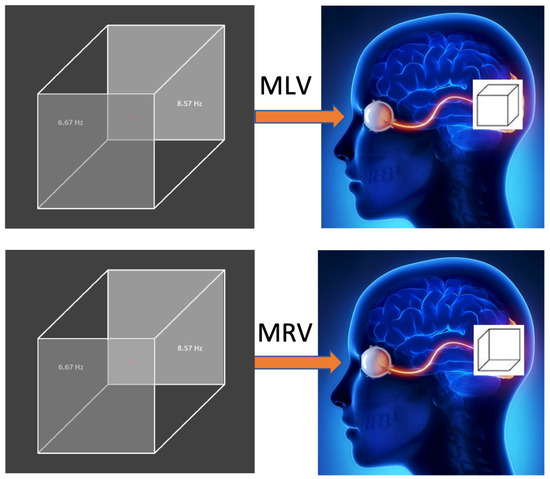
Figure 2.
Visual stimulus. In the MLV and MRV tasks, the Necker cube, with its left and right faces modulated at frequencies of 6.67 Hz and 8.57 Hz, is voluntarily perceived as left- or right-oriented, respectively. The right side illustrates the mental images generated by the brain when the subject views the same stimulus.
To minimize artifacts caused by eye movements and blinking, the subject was instructed to maintain focus on a red dot at the center of the cube and to avoid blinking during stimulus presentation. EEG preprocessing further reduced artifacts from involuntary eye movements and blinking.
Each task was repeated twice per participant, with a 2 min break between trials to allow for rest. Before each experiment, electrode conductivity was assessed to ensure optimal signal quality, maintaining electrode impedance below 10 k.
4. Experimental Data Analysis
The preliminary analysis of the recorded EEG signals was performed using the following: (i) Artifact removal to clean the raw data; (ii) Frequency spectrum analysis to identify relevant frequency regions; (iii) Wavelet analysis to determine time intervals associated with voluntary attention.
Data analysis was conducted using MATLAB (R2024b), Brainstorm [61], and BrainVision Analyzer 2.2.2 from Brain Products GmbH (Gilching, Germany). The EEG dataset utilized in this study is publicly available [62].
4.1. Artifact Removal
The analysis of the raw EEG data started with artifact removal, one of the most critical aspects of data processing. To ensure optimal processing of EEG signals, we identified and eliminated endogenous artifacts (arising from within the subject) and exogenous artifacts (external to the subject), such as interference from nearby electronic equipment, flashing lights, environmental noise, facial muscle movements, and eye blinks.
First, we executed the following steps in data preprocessing: (1) After examining the raw signals, we identified time intervals that delineated the beginning and end of the response to applied visual stimulation. (2) We minimized a continuous global current trend using the method described in [63]. This procedure improved the signal quality and facilitated the detection and correction of ocular artifacts during post-processing. (3) We removed endogenous and exogenous noise and focused on the frequencies of our stimuli. For these aims, we applied infinite impulse response (IIR) filters, specifically, 4th-order zero-phase shift Butterworth filters. Two types of filters were used: (i) band rejection (Notch Filter) to attenuate or eliminate the electrical network frequency (50 Hz in Spain) and the refresh rate of the monitor used for visual stimulation (60 Hz), with a bandwidth of 0.1 Hz, and (ii) 4th-order bandpass filter (BIF) of 4–20 Hz to concentrate on the frequencies of interest. These filters allowed us to filter out or attenuate unwanted frequency components present in the EEG signals.
Subsequently, we removed ocular artifacts, which can interfere with the detection and analysis of cortical responses as electrical activity resulting from eye movements; blinking can contaminate brain signals. To ensure that these artifacts did not distort the results or complicate the analysis, we carefully examined the brain signals associated with visual stimuli. Since the eyes behave like a dipole, with the cornea serving as the positive part and the retina as the negative part of the dipole, the identification of ocular artifacts is relatively straightforward. Vertical electro-oculogram artifacts (VEOG) and horizontal electro-oculogram artifacts (HEOG) exhibited electrical potentials ranging from 0.4 to 1.0 mV.
To mitigate the impact of ocular artifacts arising from vertical eye movements (VEOG) and lateral eye movements (HEOG) identified by inspection of raw time series, we used the Ocular Correction ICA method in BrainVision Analyzer 2.2.2, using the following algorithms:
- (i)
- Reference to frontal channels: Since our EEG equipment did not include electro-oculography electrodes, we used frontal channels (F7 and F8) as references for the ocular correction ICA. Cumulative quadratic correlation allows the precise removal of relevant components without losing neuronal information. The FP1 channel served as a common VEOG reference to detect vertical artifacts.
- (ii)
- Infomax Extended ICA algorithm: This algorithm improves the efficiency of artifact correction compared to standard ICA while preserving the neuronal signal of interest. Additionally, a Quality Control process is incorporated to ensure the validity of the obtained results. This approach enables the effective identification and reduction of ocular artifacts in EEG signals, thus facilitating the subsequent analysis of cortical responses associated with the visual stimulus by eliminating or mitigating interference from eye movements and blinks.
- (iii)
- Value trigger algorithm: This algorithm facilitated the detection of characteristic patterns, such as blinks. Blinks were identified on the basis of their absolute magnitude, with definitive blink movements determined using the correlation method. The blink detection threshold (blink value trigger) was set at 97%, which means that any value above this threshold was recognized as a blink. The selection of the 97% activation threshold for blink detection was based on experimental analysis using data from 28 participants. During threshold optimization, lower values significantly increased the rate of false positives, compromising the integrity of the neuronal signal. The 97% threshold was identified as the optimal balance between sensitivity and specificity, allowing robust identification of ocular artifacts without affecting the underlying signal. The signal correlation was established at 70% relative to a predefined blink template. This algorithm enhances detection accuracy by ensuring that triggers are only activated for signals with a high morphological similarity to a characteristic blink pattern, thereby reducing the erroneous detection of other artifacts. Additionally, a visual analysis using back-projection (Inverse ICA) was implemented as a validation method. This technique allowed the eliminated components to be projected back into the original domain, facilitating a visual inspection of the processed data. This procedure confirmed that ocular artifact suppression was performed selectively, preserving relevant neuronal activity while minimizing EEG signal distortion.These values were experimentally determined by considering their influence on attenuating the signal of interest in the spectral regions of and in the occipital lobes (O1, Oz, O2 channels).
Lastly, we conducted ICA to find the optimal unmixing matrix to separate independent sources using statistical methods. To assess component independence, methods such as Maximum Negentropy, Kurtosis, Maximum Likelihood, and Mutual Information were employed. The optimization process for the optimal unmixing matrix ended when the maximum time independence of the components was achieved within a maximum number of steps or iterations. For this process, the extended nondeterministic INFOMAX algorithm with a maximum of 512 steps was selected as the optimal configuration. This ICA training method was adjusted after each convergence step to enhance signal separation. Convergence was deemed achieved when the algorithm reached a stable solution, favoring Independent Components (ICs) with Kurtosis (K) values greater than 0 (indicating components with a non-Gaussian distribution) and less than 0 for noise, such as electrical network noise.
Following decomposition into ICs, quality control was performed by examining the number of steps used in decomposition of the ICs and comparing them with components initially flagged as possible ocular artifacts during visual inspection of the raw time series. As a final step, an inverse ICA of ICs and topographic retroprojection were performed to determine the brain lobes to which these possible signals corresponded. The analysis involved a comprehensive evaluation of the properties of IC, including their waveforms over time, energy, and kurtosis (, , ).
It should be noted that ICA was performed on full-rank data without any preprocessing steps that could affect its rank [64].
4.2. Spectral Analysis
The FFT method enables the examination of a signal’s frequency spectrum, which is essential for identifying frequency tags associated with flickering visual stimuli. In this study, we focus on the tag frequencies corresponding to the two perceived orientations of the Necker cube: for the left-oriented cube and for the right-oriented cube.
To ensure optimal analysis resolution, we implemented an FFT algorithm designed to operate on power-of-2 segmentations. The EEG signals were segmented into 30 s trials based on the duration of each task (MI, MLV, or MRV). Following preprocessing and artifact removal, the FFT was computed for 20 s frames with a 1 s overlap to reduce noise. This configuration maximized spectral resolution, allowing for efficient and precise signal decomposition in the frequency domain. As a result, we could efficiently identify the spectral characteristics associated with each cube orientation when analyzing EEG signals.
The FFT spectra of the MI, MLV, and MRV tests are shown in Figure 3. Distinct spectral peaks can be observed near the modulation frequencies within the ranges and . The brain does not respond on discrete frequencies due to two factors: (i) the modulation signal is not harmonic, and (ii) slight variation in the modulation signal occurs throughout the experiment, influenced by computer load and memory fluctuations.

Figure 3.
FFT spectra of preprocessed EEG from the O1 channel during (a) MI, (b) MRV, and (c) MLV tasks. The vertical dashed lines bound frequency regions of interest ( and ), representing the brain response to stimulus modulation.
By comparing the spectrum obtained for involuntary attention (MI) shown in Figure 3a with the spectra for voluntary attention to the left-oriented cube (MLV), shown in Figure 3b, and to the right-oriented cube (MRV), shown in Figure 3c, it can be observed that the spectral amplitude at dominates the amplitude at when the subject perceives the cube as left-oriented (Figure 3b), and the spectral amplitude at dominates the amplitude at when the subject perceives the cube as right-oriented.
4.3. Wavelet Analysis
The wavelet analysis provides a detailed view of how spectral energy fluctuates over time, offering insights into the dynamic nature of decision-making processes as captured through neurophysiological data. The wavelet power spectrum serves as a quantifiable metric, enabling the precise measurement of these temporal changes [43,65,66,67,68,69,70].
While the spectra depicted in Figure 3 were computed over the entire 30 s EEG time series, it is important to note that sustained attention is not maintained uniformly throughout this period. To identify specific time windows during which attention was focused, we employed wavelet analysis. Using the Morlet wavelet, we were able to pinpoint intervals where attention was predominantly directed toward one interpretation of the cube over another.
The temporal dynamics of the cube’s orientation interpretation were explored through continuous wavelet transform (CWT) analysis, implemented using the Brainstorm software (version 3.4.0.0). This method allowed us to investigate how attention shifted over time, revealing the moments when the subject focused attention on specific interpretations of the cube. By leveraging wavelet analysis, we gained a more granular understanding of the temporal patterns underlying attentional processes during the task.
Figure 4a,b depict the variations in wavelet energy corresponding to figurative attention directed towards the left (MLV) and right (MRV) cube orientations, respectively. The wavelet energy was calculated using the following equation:
where the asterisk (*) denotes the complex conjugate, represents the analyzed EEG signal, and is the complex-valued Morlet wavelet, chosen as the mother wavelet. The Morlet wavelet is defined as follows:
with being the central frequency of the Morlet wavelets, the imaginary unit, and representing the time shift parameter. This formulation allows for a precise analysis of the temporal and spectral characteristics of the EEG signal, capturing the dynamic shifts in attention during the task.

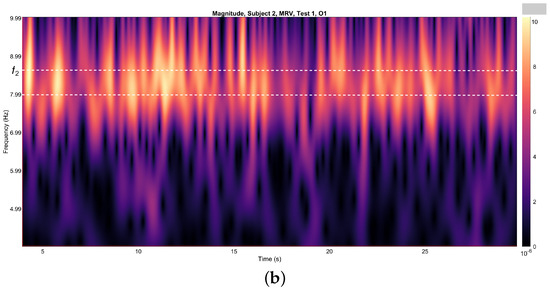
Figure 4.
Wavelets from channel O1, illustrating the spectral energy associated with figurative attention directed towards (a) left-cube (MLV) and (b) right-cube (MRV) orientations. The peak wavelet energy is observed within distinct frequency regions: (a) when the subject perceives the cube as left-oriented, and (b) when the subject perceives the cube as right-oriented. The frequency ranges and are demarcated by horizontal dashed lines, highlighting the specific bands where attentional focus is most pronounced.
It is evident that the prominence of specific components corresponds to the subject’s directed attention towards either the left or right orientation of the cube. The spectral component at is dominant when the subject perceives the cube as left-oriented (Figure 4a), while prevails when the cube is interpreted as right-oriented (Figure 4b). As shown in Figure 4, spectral energy at dominates during the time interval seconds in the MLV test, whereas spectral energy at dominates during the interval seconds in the MRV test. In the subsequent analysis, connectivity is calculated within these identified time intervals.
5. Graph Construction
In this section, we construct brain connectivity networks associated with figurative attention using three widely used measures: coherence, cross-correlation, and mutual information. These measures allow us to examine how attention influences both connectivity and disconnectivity between different brain regions. During an attentive state, connectivity between some brain areas may increase, while in others, it may decrease. To capture this dynamics, we construct separate graphs for positive and negative connectivity changes.
The connectivity measures were calculated for every pair of signals recorded from 16 EEG channels within the frequency ranges and , as identified from the FFT spectra. Additionally, from the wavelet analysis (Figure 4), we selected time intervals of seconds for attention to the let-oriented cube and seconds for attention to the right-oriented cube.
Connectivity C between brain regions was calculated for signals from each electrode pair using Equations (9)–(11) for MI, MLV, and MRV tests in both the and spectral regions. Subsequently, we determined positive and negative changes in connectivity associated with attention as follows:
To evaluate connectivity in the constructed graphs, we utilized the ’conncomp’ function in MATLAB. This function identifies connected components in an undirected graph, providing a quantitative measure of network connectivity. It assigns each node a connected component identifier, allowing us to determine the total number of connected components within the graph.
5.1. Connectivity Graphs Based on Coherence
To construct connectivity graphs, we first calculate coherence between signals from each pair of electrodes for the MI, MLV, and MRV tests in the and spectral regions using Equation (9). Next, we computed the differences and associated with attention using Equation (14). The resulting labeled graphs of coherence () and anticoherence () are displayed in Figure 5 and Figure 6, respectively. The corresponding coherence matrices are provided in Figure A1 and Figure A2 in Appendix B.
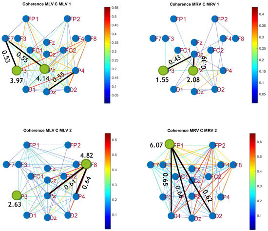
Figure 5.
Connectivity graphs based on coherence in the (upper raw) and (lower raw) frequency regions, associated with (left column) left-cube attention () and (right column) right-cube attention (). Bold lines highlight the links with the largest coherence differences (Max ), which are displayed next to the corresponding links. Orange dots denote the nodes with the highest sums of their link weights, indicated next to these nodes.
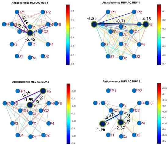
Figure 6.
Disconnectivity graphs based on anticoherence in the (upper raw) and (lower raw) frequency regions, associated with (left column) left-cube attention () and (right column) right-cube attention (). Bold lines highlight the links with the largest negative coherence differences (Min ). Violet dots denote the nodes with the lowest sums of their link weights, indicated next to these nodes.
The colors in Figure 5 and Figure 6 represent the numerical weights of the links, illustrating coherence differences () resulting from shifts in attention. The strongest links are emphasized with bold lines and labeled with their corresponding coherence differences. We also calculated the total sum of link weights for each node, displaying these values next to the nodes with the highest sums, which are marked with orange dots. In contrast, nodes with the lowest (negative) labels are indicated with violet dots.
A significant contrast in coherence patterns emerges between frequency regions and . When attention is directed toward the left-cube orientation, coherence increases prominently between the left anterior frontal (F7) and midline parietal (Pz) and left parietal (P3) lobes at (upper left panel, Figure 5). In contrast, at , coherence increases symmetrically in the right hemisphere, particularly between the right anterior frontal (F8), midline parietal (Pz), and right parietal (P4) lobes (lower left panel, Figure 5). These findings suggest that the anterior frontal lobes play a crucial role in figurative attention.
For right-cube attention, coherence increases between the left parietal (P3) and midline central (Cz) lobes, as well as between the midline parietal (Pz) and midline central (Fz) lobes at (upper right panel, Figure 5). However, at , coherence significantly increases between the occipital cortex (O1, Oz, O2) and the left prefrontal lobe (FP1) (lower right panel, Figure 5). These observations suggest that the left prefrontal cortex may play a key role in processing right-cube orientation, as the frequency is applied to the right face of the cube. Our findings align with prior studies, such as Al-Nafjan and Aldayel [37], which also reported attention-related activity in the prefrontal and parietal cortices.
A critical aspect of these results is the simultaneous decrease in coherence between certain brain regions, indicating that attention not only strengthens specific neural connections but also selectively disconnects others. Given the brain’s energy-intensive nature, this redistribution likely reflects an optimization of cognitive resources. Figure 6 visualizes this selective disconnectivity through anticoherence graphs.
The results reveal a notable reduction in coherence at between the midline central (Cz) and left frontal (F3) lobes, as well as between the midline central (Cz) and left prefrontal (FP1) lobes during left-cube attention (upper left panel, Figure 6). At , coherence decreases between the midline frontal (Fz) and right prefrontal (FP2) lobes, as well as between the left frontal (F3) and right prefrontal (FP2) lobes (lower left panel, Figure 6). These results suggest that the central cortex is a primary region of disconnectivity and that the reduction in prefrontal-central connectivity facilitates increased parietal-frontal interactions.
For right-cube attention, a different pattern emerges. At , coherence decreases between the anterior frontal lobes (F7 and F8), while at , coherence decreases between the left parietal (P3) and midline central (Cz) lobes, as well as between the midline parietal (Pz) and midline central (Cz) lobes. Notably, the nodes (P3, Pz) and links to Cz with the greatest coherence reduction at (lower right panel, Figure 6) coincide with those showing the greatest coherence increase at (upper right panel, Figure 5). This suggests a frequency-dependent reorganization, where attention to the right-cube orientation enhances coherence in these regions at while simultaneously reducing coherence at .
Table 1 summarizes the graph-based analysis of brain connectivity, listing the two highest positive and negative coherence differences (link weights) and their corresponding lobes.

Table 1.
Maxima and minima coherence differences.
5.2. Connectivity Graphs Based on Cross-Correlation
To construct connectivity graphs based on cross-correlation, we first computed cross-correlation between EEG signals from each pair of channels using Equation (10), then calculated attention-induced differences using Equation (14). The resulting graphs, shown in Figure 7 and Figure 8, depict regions of the increasing and decreasing cross-correlation, respectively. Additionally, the corresponding cross-correlation matrices, presented in Appendix B (Figure A3 and Figure A4), provide a detailed numerical representation of these connectivity changes.
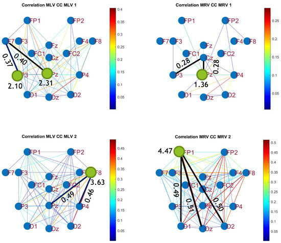
Figure 7.
Connectivity graphs based on cross-correlation in the (upper raw) and (lower raw) frequency regions, associated with (left column) left-cube attention () and (right column)

Figure 8.
Disconnectivity graphs based on anticorrelation in the (upper raw) and (lower raw) frequency regions, associated with (left column) left-cube attention () and (right column) right-cube attention (). Bold lines highlight the links with the largest negative cross-correlation differences (Min ). Violet dots denote the nodes with the lowest sums of their link weights, indicated next to these nodes.
By comparing Figure 5 and Figure 6 with Figure 7 and Figure 8, we observe a strong similarity between the connectivity patterns derived from cross-correlation and coherence measures. Specifically, the links showing the maximum increases and decreases in cross-correlation closely match those for coherence. This agreement between connectivity measures, based on both temporal and spectral analyses, provides strong validation for the robustness of our findings.
Table 2 summarizes the results of the brain connectivity analysis based on cross-correlation. The table presents the two largest positive and negative correlation differences (link weights) along with the corresponding brain regions.
Table 2.
Maxima and minima cross-correlation differences.
5.3. Connectivity Graphs Based on Mutual Information
The third connectivity measure explored in this study, mutual information, was calculated using Equation (11). The differences in mutual information induced by attention were computed using Equation (14). The resulting graphs depicting the attention-induced changes in mutual information are shown in Figure 9 and Figure 10. Additionally, the corresponding mutual information matrices are provided in Appendix B, specifically in Figure A5 and Figure A6, offering a detailed numerical representation of these connectivity changes.

Figure 9.
Connectivity graphs based on mutual information in the (upper raw) and (lower raw) frequency regions, associated with (left column) left-cube attention () and (right column) right-cube attention (). Bold lines highlight the links with the largest mutual information differences (Max ), which are displayed next to the corresponding links. Orange dots denote the nodes with the highest sums of their link weights, indicated next to these nodes.
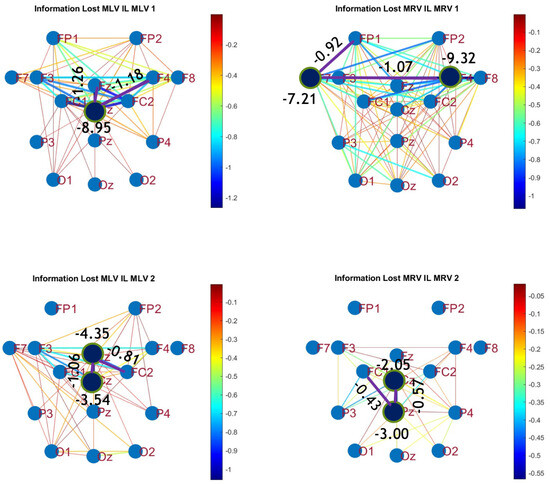
Figure 10.
Disconnectivity graphs based on mutual information loss in the (upper raw) and (lower raw) frequency regions, associated with (left column) left-cube attention () and (right column) right-cube attention (). Bold lines highlight the links with the largest negative mutual information differences (Min ). Violet dots denote the nodes with the lowest sums of their link weights, indicated next to these nodes.
Table 3 summarizes the brain connectivity analysis results based on mutual information. It highlights the two largest positive and negative mutual information differences (link weights) along with their corresponding brain regions, providing insight into the most significant connectivity changes induced by attention shifts.
Table 3.
Maxima and minima mutual information differences.
A strong correspondence can be observed among the connectivity graphs based on coherence, cross-correlation, and mutual information. Although some variations exist in the links with the highest weights, the nodes with the maximum and minimum labels largely overlap across all connectivity measures. This consistency further validates the robustness of our approach in capturing attention-related connectivity changes in the brain.
The shared features across different connectivity measures can be explored using hypergraphs. In the following section, we describe the process of constructing attention hypergraphs.
6. Hypergraph Construction
Hypergraph analysis provides a simplified and more generalized representation of the brain network. Instead of relying on the twelve individual graphs presented in the previous section, we can construct four hypergraphs using the summarization technique described in Section 2.2.
To construct the hypergraphs, we follow these steps:
- (1)
- Compute the label of every node i for each connectivity measure using Equation (2) (Lab ).
- (2)
- From the probability distribution of all n labels for each connectivity measure found the mean and standard deviation .
- (3)
- Calculate threshold value for each connectivity measure (“+” for , “−” for ).
- (4)
- Using the threshold value, determine whether a change in connectivity is significant or not. The change is significant if the label .
- (5)
- Using the summarization technique described in Section 2.2 remove insignificant nodes whose labels are smaller than the threshold value. Weak changes in connectivity are considered as brain noise and are not related to attention.
- (6)
- Construct incident matrices using Equation (5).
The probability distributions for each connectivity measure are presented in Figure A7, Figure A8 and Figure A9 in Appendix C. One can also find there the values of means (M), standard deviations (), and thresholds (), which are summarized in Table A1.
6.1. Simple Hypergraphs
Using the algorithm described above, we constructed four hypergraphs, denoted as . Two of these hypergraphs () correspond to attention directed toward the left-cube orientation, while the other two () correspond to attention directed toward the right-cube orientation. Hypergraphs and are constructed for frequency region , while and are constructed for .
Each hypergraph contains six hyperedges (): and represent coherence and anticoherence, and represent correlation and anticorrelation, and and represent mutual information and information loss, respectively.
The constructed hypergraphs are visualized in Figure 11, Figure 12, Figure 13 and Figure 14 in three distinct forms: as a bipartite graph (left panels), a Venn diagram (middle panels), and a brain map (right panels). The correspondence between node numbers and EEG channels is provided in Table 4.

Figure 11.
Hypergraph associated with left-cube attention for , presented as a bipartite graph (left), a Venn diagram (middle), and a brain map (right). The upper Venn diagram (, , ) indicates deactivation of central area, while the lower one (, , ) depicts activation of occipital-parietal area.
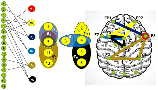
Figure 12.
Hypergraph associated with left-cube attention for , presented as a bipartite graph (left), a Venn diagram (middle), and a brain map (right). The right Venn diagram (, , ) indicates deactivation of left frontal and right prefrontal lobes, while the left one (, , ) depicts activation of parietal, right anterior, and left prefrontal lobes.

Figure 13.
Hypergraph associated with right-cube attention for , presented as a bipartite graph (left), a Venn diagram (middle), and a brain map (right). The left Venn diagram (, , ) indicates deactivation of frontal cortex, while the right one (, , ) depicts activation of parietal area.
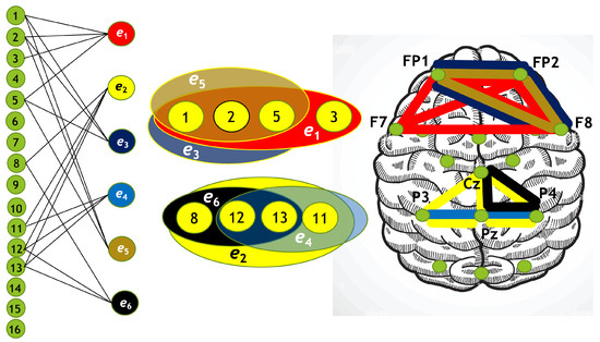
Figure 14.
Hypergraph associated with right-cube attention for , presented as a bipartite graph (left), a Venn diagram (middle), and a brain map (right). The lower Venn diagram (, , ) indicates deactivation of central-parietal area, while the upper one (, , ) depicts activation of frontal cortex.
Table 4.
Correspondence of node numbers to EEG channels.
A hypergraph size is the number of hyperedges (in our case ), and the order of a hypergraph is the number of vertices. The degrees of hyperedges and the orders of the hypergraphs are summarized in Table 5.
Table 5.
Degrees of hyperedges and orders of hypergraphs.
6.2. Multilayer Hypergraphs
The hypergraphs of figurative attention can be represented as multilayer hypergraphs, where each layer corresponds to a hypergraph capturing increased or decreased connectivity at a specific frequency. This approach allowed us to consolidate four separate hypergraphs into two four-layer hypergraphs, one for left-cube attention and another one for right-cube attention. The resulting four-layer hypergraphs are presented in Figure 15 and Figure 16.
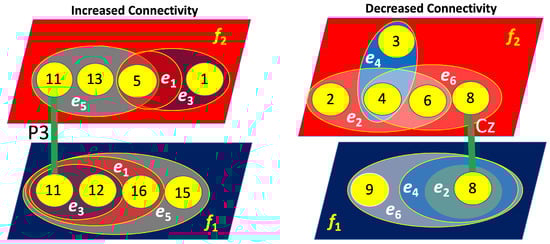
Figure 15.
Four-layer hypergraphs representing brain connectivity (left layers) and disconnectivity (right layers) associated with left-cube attention. The lines indicate inter-layer connections, with the corresponding channels responsible for these links labeled near the lines.

Figure 16.
Four-layer hypergraphs representing brain connectivity (left layers) and disconnectivity (right layers) associated with right-cube attention. The lines indicate inter-layer connections, with the corresponding channels responsible for these links labeled near the lines.
As shown in Figure 15, for the left-cube attention, the layers exhibiting increased and decreased connectivity are not interconnected, meaning they do not share common nodes. Notably, the layers associated with increased connectivity at and are primarily linked through the left parietal lobe (P3). Conversely, the layers related to decreased connectivity at and are mainly connected via the central lobe (Cz). These nodes demonstrate the most significant increase and decrease in connectivity, respectively.
In contrast, Figure 16 reveals that for the right-cube attention, the layers of increased and decreased connectivity are strongly interconnected. Specifically, the layer with increased connectivity at is linked through three nodes (FP1, F7, and F8) to the layer of decreased connectivity at . Simultaneously, the layer of increased connectivity at is connected via three nodes (Pz, P3, and P4) to the layer of decreased connectivity at . This indicates a reciprocal relationship, where an increase in connectivity at is accompanied by a decrease at , and vice versa.
6.3. Dual Clique Expansions
The high-order interactions shown as the hypergraphs in Figure 11, Figure 12, Figure 13 and Figure 14 can also be presented in the form of dual clique expansions shown in Figure 17 and Figure 18. As was defined in Section 2.1, a clique expansion is a transformation where each hyperedge is replaced by a clique connecting all vertices within that hyperedge. This is commonly used to approximate hypergraphs using graphs. To construct dual clique expansions of , we first created dual hypergraphs and then performed clique expansions on , meaning that each hyperedge (which corresponds to a vertex in ) is expanded into a clique. As a result, we created new hypergraphs where hyperedges correspond to cliques in .

Figure 17.
Dual clique expansions of hypergraphs associated with left-cube attention at (left) and (right) .

Figure 18.
Dual clique expansions of hypergraphs associated with right-cube attention at (left) and (right) .
The analysis of the dual clique expansions , presented in Figure 17 and Figure 18, reveals distinct connectivity patterns among brain regions. Specifically, all connectivity measures—coherence, correlation, and mutual information—are mutually connected through the nodes . Conversely, all disconnectivity measures—anticoherence, anticorrelation, and information loss—also form a mutually connected structure. In other words, these results highlight the brain regions (edges in these graphs) that predominantly contribute to both increasing and decreasing connectivity associated with figurative attention.
For both left- and right-cube attention, the primary contributors to increased connectivity are the parietal region (P3, Pz, P4) at and the refrontal and frontal regions (FP1, FP5, F8) at . In contrast, decreased connectivity is primarily driven by the centro-frontal region (Cz, F7, F8) at and the fronto-parietal region (Fz, F3, Cz, P3, Pz, P4) at .
Additionally, an inverse relationship emerges between different frequency bands and cube percepts. The parietal cortex (P3, Pz, P4), which enhances connectivity at , becomes disconnected at during right-cube attention. Similarly, the right frontal region (F8), which supports increased connectivity during left-cube attention task (MLV) at , disconnects at during the right-cube attention task (MRV). This suggests an antiphase activation-deactivation dynamics, where increased connectivity for one percept at a specific frequency coincides with decreased connectivity for the alternative percept at another frequency.
7. Discussion
Hypergraphs have been extensively studied and applied in network analysis, including node classification [71], community detection [72], and link prediction [73]. In neuroscience, hypergraphs, as a generalization of the graph theory, provide a more sophisticated framework for modeling brain connectivity by capturing high-order interactions among multiple brain regions [74]. Recent studies [21] have constructed hypergraphs using functional and structural connectivity as hyperedges. In contrast, we created hypergraphs based on three connectivity measures (coherence, cross-correlation, and mutual information) and three disconnectivity measures (anticoherence, anticorrelation, and information loss). Additionally, we employed sparsification techniques to remove less significant nodes, reducing noise and enhancing functional connectivity interpretation.
By incorporating hypergraph theory into EEG-based functional connectivity analysis, our method provides a novel perspective on understanding attention and its neural correlates. Hypergraph-based models enable a subject-level representation of high-order relationships, facilitating a more refined analysis of individual differences in cognitive function. This has significant implications for identifying biomarkers of attention-related disorders and advancing personalized cognitive assessments. Recent advancements in deep learning have further amplified the potential of hypergraph-based models. Ji et al. [19] introduced the hypergraph attention network (FC-HAT), while Bi et al. [75] developed the hypergraph structural information aggregation generative adversarial network (HSIA-GAN) model for functional connectivity analysis. These models dynamically construct functional connectivity networks, extract abnormal connectivity patterns, and identify critical biomarkers for neurodevelopmental and neurodegenerative disorders.
Our hypergraph analysis reveals that hyperedges associated with increased and decreased connectivity are spatially distinct and localized in different brain regions, depending on both the cognitive task and frequency. Since attention to the left-cube orientation is linked to increased spectral energy at , the hypergraph in Figure 11 highlights the key nodes involved in this cognitive process. Notably, the occipital-parietal cortex emerges as a central hub for functional connectivity, whereas the central cortex plays a predominant role in disconnectivity.
An intriguing observation is the frequency-dependent nature of brain region activity: nodes that exhibit increased connectivity at one frequency tend to show decreased connectivity at another. For instance, the left parietal lobe (P3), which is highly active at (Figure 11), demonstrates reduced activity at (Figure 12), suggesting a dynamic reconfiguration of neural networks in response to different attentional states.
A similar pattern is evident during right-cube attention. The hypergraph in Figure 14 indicates that the frontal cortex plays a central role in connectivity, while the central-parietal cortex is predominantly associated with disconnectivity. This observation aligns with the fact that right-cube attention corresponds to increased spectral energy at . Once again, the same brain regions exhibit frequency-dependent activation and deactivation, reinforcing the notion that attentional shifts are accompanied by distinct neural reorganization patterns across different frequency bands. Specifically, for right-cube attention, the frontal and prefrontal cortices demonstrate increased activity at (Figure 14) but reduced activity at (Figure 13). In contrast, the parietal cortices show the opposite trend, increasing their activity at (Figure 13) while decreasing at (Figure 14).
Our study also confirms the crucial role of the prefrontal and parietal regions in attentional processes, consistent with findings from previous research. Numerous studies have investigated the neural correlates of attention using EEG-based approaches with varying methodological frameworks and analytical techniques. While these studies have provided valuable insights, their reliance on traditional graph-theoretical and spectral-based methods limits their ability to capture the full complexity of brain connectivity dynamics. In contrast, hypergraph-based approaches offer a richer framework that better represents the multi-dimensional and frequency-specific interactions underlying attentional mechanisms.
Early studies on EEG-based attention research [76,77,78] examined delta- and alpha-wave amplitudes as indicators of attention. While these studies laid the groundwork for EEG-based attentional analysis, they relied on a univariate spectral approach. Moreover, their interpretations—linking delta and alpha activity primarily to low awareness—may be overly simplistic. Fahimi et al. [79] explored EEG-based neural markers of attention in elderly participants, correlating frontal EEG features with reaction times. Although their work underscores the potential of single-channel EEG analysis, it overlooks the distributed and interconnected nature of attentional networks. Similarly, Wan et al. [80] computed spectral power ratios (, , ) for attention recognition—an approach that, while common, treats frequency bands as isolated rather than interdependent components of a complex system. In contrast, hypergraph-based analysis offers a more nuanced perspective by revealing interactions between different connectivity measures at specific frequencies. It addresses these limitations by capturing higher-order connectivity patterns across multiple regions and frequencies simultaneously.
Machine learning has also been widely applied to EEG-based attention detection. Several studies [81,82,83] used various classification techniques (e.g., Support Vector Machine (SVM), Linear Discriminant Analysis (LDA), Naive Bayes) to distinguish attentional states. While these methods are powerful for predictive modeling, they often lack interpretability regarding the underlying neural mechanisms. A hypergraph representation provides a more interpretable structure by modeling attention states as overlapping neural communities rather than treating EEG features as independent inputs for classification. Moreover, passive brain–computer interface (BCI) studies, such as those by Aci et al. [84], aimed to classify mental states (e.g., passive attention, disengagement, drowsiness) using EEG. However, most BCI-based attention-monitoring approaches rely on traditional feature extraction methods that fail to capture the full spectrum of interactions within attentional networks. Hypergraphs enhance these approaches by integrating multi-scale and multi-frequency relationships, leading to more robust and generalizable attention-monitoring systems.
While prior studies have made significant contributions to EEG-based attention research, they are often constrained by their methodological frameworks, which rely on simplistic spectral analyses, pairwise connectivity measures, and black-box machine learning models. By contrast, hypergraph-based approaches offer a more comprehensive representation of attentional processes, accounting for higher-order interactions, multi-frequency dynamics, and network-wide connectivity patterns.
It is essential to highlight that while the various hypergraph representations explored in this study offer similar insights into brain connectivity, each captures distinct aspects of neural dynamics. These differences contribute to a more comprehensive understanding of the mechanisms underlying figurative attention. Our findings suggest that figurative attention involves a dynamic redistribution of neural resources, with specific brain regions alternating between connectivity and disconnectivity based on cognitive demands and frequency. This reorganization reflects the brain’s ability to adapt its functional networks, ensuring efficient information processing across different attentional states.
The observed frequency-dependent connectivity shifts underscore the importance of considering frequency-specific interactions in functional brain network analysis. Traditional graph-based methods may overlook these nuances, whereas hypergraph-based approaches provide a powerful framework for capturing the complex, higher-order dependencies that shape attentional processes. By integrating multiple connectivity measures within a hypergraph structure, this method offers a richer, more holistic representation of neural interactions.
Future research could extend this approach to other cognitive domains, such as working memory or decision-making, to further investigate the intricate dynamics of brain connectivity across different tasks and states.
8. Conclusions
This study presents a comprehensive hypergraph-based analysis of functional brain connectivity during figurative attention to an ambiguous visual stimulus, integrating coherence, cross-correlation, and mutual information from EEG data. Our findings support the hypothesis that figurative attention engages cortico–cortical interactions, with hypergraph representations revealing distinct frequency-dependent activation and deactivation patterns across brain regions. Notably, the parietal, frontal, and prefrontal lobes play a key role in integrating information, highlighting their functional specialization and dynamic reconfiguration in attentional processing. However, while these regions facilitate efficient cognitive functions, some information may be lost in the central cortex, underscoring the complexity of neural information processing.
By leveraging a frequency-tagging approach in the context of the Necker cube illusion, we identified distinct connectivity patterns corresponding to different cube orientations. Our results emphasize the role of bilateral cortico–cortical interactions and suggest the existence of integrated processing hubs that coordinate visual attention. Hypergraph analysis, extending beyond traditional graph-based methods, provided novel insights into higher-order relationships between multiple brain regions, offering a more comprehensive understanding of dynamic neural interactions.
The methodology developed in this study—incorporating three connectivity and three disconnectivity measures—enabled the identification of higher-order relationships among brain regions, facilitating a more precise characterization of functional connectivity networks underlying figurative attention. This multivariate approach allowed us to construct connectivity difference matrices, revealing both new connections induced by sustained attention and disconnections due to decreased connectivity. Additionally, by applying a sparsification method based on statistical thresholds, we filtered out spurious or noisy connections, enhancing the robustness and interpretability of our functional connectivity network.
Beyond its theoretical implications, this methodological framework holds promise for practical applications in cognitive neuroscience, attention monitoring, and the clinical assessment of attention-related disorders. While this proof-of-concept study is based on a single subject, it establishes a foundation for future large-scale investigations into the neural mechanisms underlying ambiguous visual perception and attentional control.
Although previous studies have explored frequency correlations and proposed biophysical models of neural interactions, our findings highlight the need for further studies investigating the mechanisms linking different frequency-dependent processes. A more refined hypergraph analysis, focusing on smaller neural ensembles or specific regions of interest, could provide deeper insights into the intricate dynamics of brain connectivity. This study lays essential groundwork for advancing our understanding of brain network dynamics and their role in cognitive function.
Hypergraphs provide a powerful framework for modeling high-order interactions in EEG-based functional connectivity networks. Our findings emphasize the importance of incorporating connectivity and disconnectivity measures in hypergraph construction, enabling a more comprehensive understanding of individual differences in attention and cognitive processing. Future research should focus on further refining hypergraph learning algorithms, integrating dynamic hypergraph representations, and expanding applications to clinical populations for biomarker discovery and personalized interventions in cognitive and psychiatric disorders.
While our findings demonstrate the potential of hypergraph-based models for capturing the complex neural dynamics underlying attention, several challenges must be addressed before this approach can be fully integrated into clinical practice. Key obstacles include the need for larger and more diverse datasets, enhanced interpretability of hypergraph representations, and rigorous validation across a broader range of cognitive tasks and populations. Overcoming these challenges will be essential for ensuring the reliability and applicability of hypergraph-based methods in both research and real-world settings.
Despite these hurdles, our study represents a significant step toward more precise and individualized assessments of brain function. By leveraging a hypergraph-based connectivity analysis, we provide a novel framework that moves beyond traditional graph-theoretic approaches, offering a richer and more nuanced understanding of attentional processes. Future research should focus on refining these models, integrating them into EEG analysis pipelines, and exploring their potential for real-time applications in cognitive neuroscience and clinical diagnostics. Ultimately, this work lays the foundation for more advanced and interpretable assessments of brain connectivity, with implications for both fundamental research and applied neurotechnology.
Author Contributions
A.N.P.: conceptualization, methodology, investigation, formal analysis, validation, visualization, writing—original draft preparation, supervision; N.P.S.: investigation, investigation, formal analysis, visualization; W.E.P.d.l.V.: investigation, data curation, software, methodology, formal analysis, writing; R.J.-R.: investigation, validation, review and editing. All authors have read and agreed to the published version of the manuscript.
Funding
This research received no external funding.
Institutional Review Board Statement
The study was conducted in accordance with the Declaration of Helsinki, and approved by the Ethics Committee of the Universidad Politécnica de Madrid (Approval Code: 2020-096).
Informed Consent Statement
Informed consent was obtained from the subject involved in the study.
Data Availability Statement
The data presented in this study are openly available in Google Drive at https://drive.google.com/drive/folders/1_PHVe2rsr4ohWufccE7oYNKNAEOB37BA (accessed on 5 February 2025).
Conflicts of Interest
The authors declare no conflicts of interest.
Appendix A. Data Acquisition Details
EEG signal acquisition followed a semi-automatic protocol that integrated manual event activation with automated processing via BrainVision Recorder 1.27 software. The procedure included the following steps:
- (1)
- Recording (triggers): Triggers were configured within the BrainVision Recorder program, manually activated by the researcher through keypresses at the start and end of each recording. These triggers were labeled in the raw EEG signals, allowing for later identification of the analysis window.
- (2)
- Start and End Margins: The recording included a 3 s margin before the start and 3 s after the end, resulting in a total window of 36 s, of which 30 s corresponded to the experimental period of interest.
- (3)
- Justification for Temporal Margins: The implementation of these temporal margins aimed to minimize artifacts associated with the initiation and termination instructions of the task. The participant took approximately 3 s to process the start instruction, which could introduce transient artifacts in the signal. Similarly, the recording automatically stopped at 36 s with the trigger, reducing the variability associated with manual intervention in the recording termination.
- (4)
- Preprocessing Segmentation: During preprocessing, the 30 s window was extracted, discarding the first and last 3 s to eliminate transient artifacts and ensure that the analysis was performed on stationary data, free from transient influences.This methodological approach reduced variability and increased data reliability without requiring additional hardware for event activation.
Appendix B. Connectivity Matrices
The matrices of the explored connectivity measures are presented in Figure A1, Figure A2, Figure A3, Figure A4, Figure A5 and Figure A6.

Figure A1.
Increasing coherence () associated with figurative attention to (left panels) left cube orientation and (right panels) at frequencies (upper raw) and (lower raw) .
Figure A1.
Increasing coherence () associated with figurative attention to (left panels) left cube orientation and (right panels) at frequencies (upper raw) and (lower raw) .
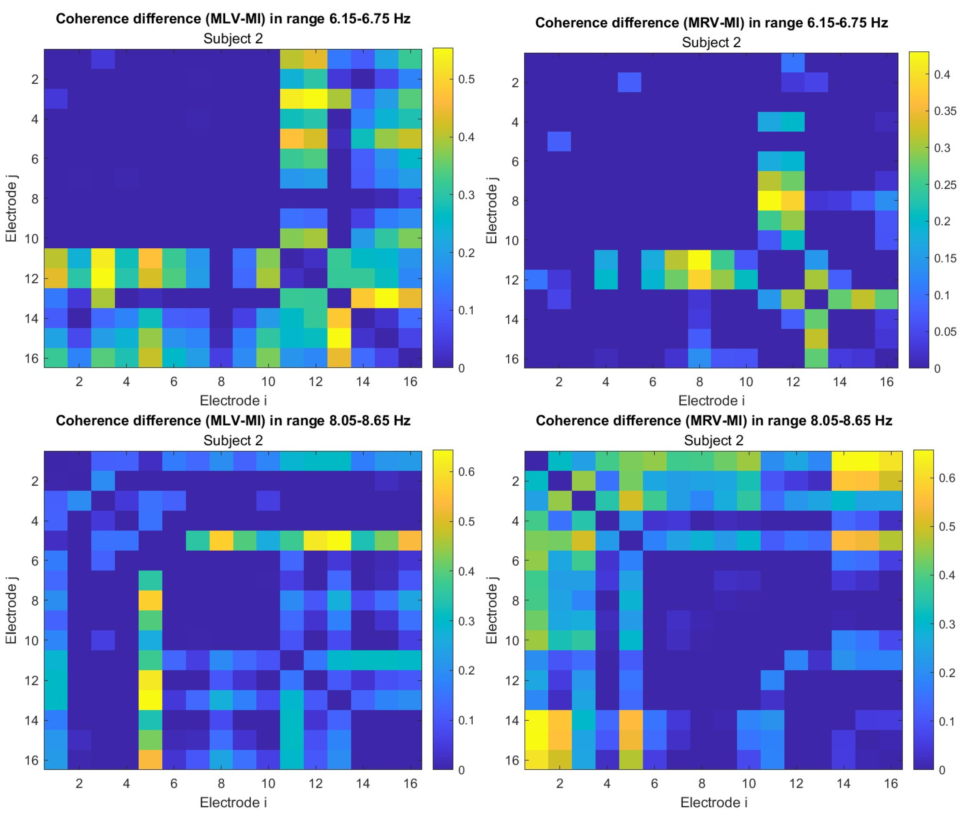

Figure A2.
Decreasing coherence () associated with figurative attention to (left panels) left cube orientation and (right panels) at frequencies (upper raw) and (lower raw) .
Figure A2.
Decreasing coherence () associated with figurative attention to (left panels) left cube orientation and (right panels) at frequencies (upper raw) and (lower raw) .
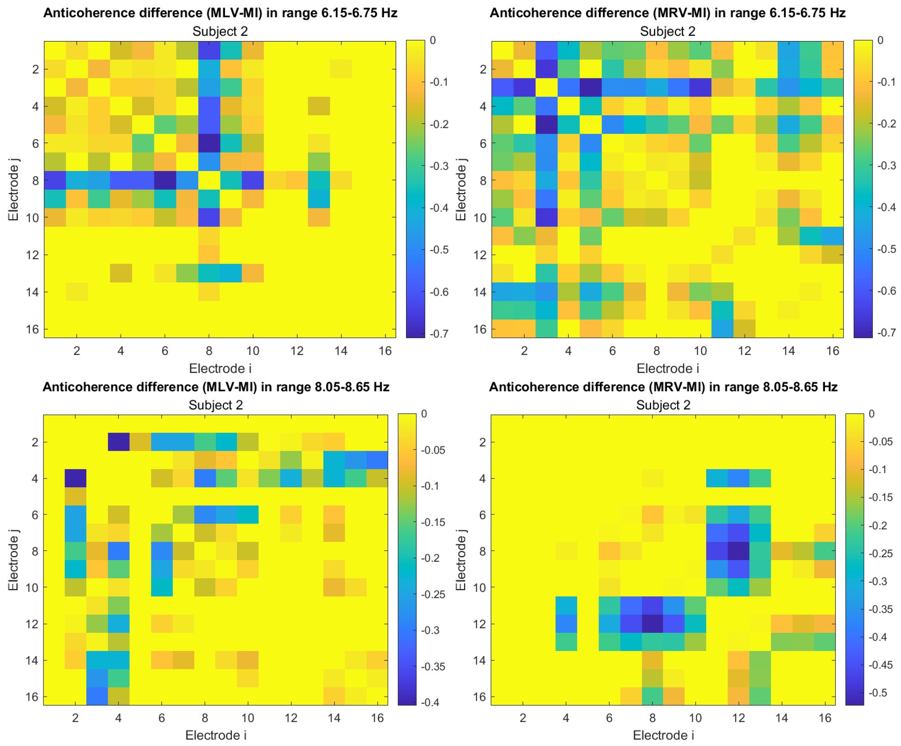

Figure A3.
Increasing cross-correlation () associated with figurative attention to (left panels) left cube orientation and (right panels) at frequencies (upper raw) and (lower raw) .
Figure A3.
Increasing cross-correlation () associated with figurative attention to (left panels) left cube orientation and (right panels) at frequencies (upper raw) and (lower raw) .
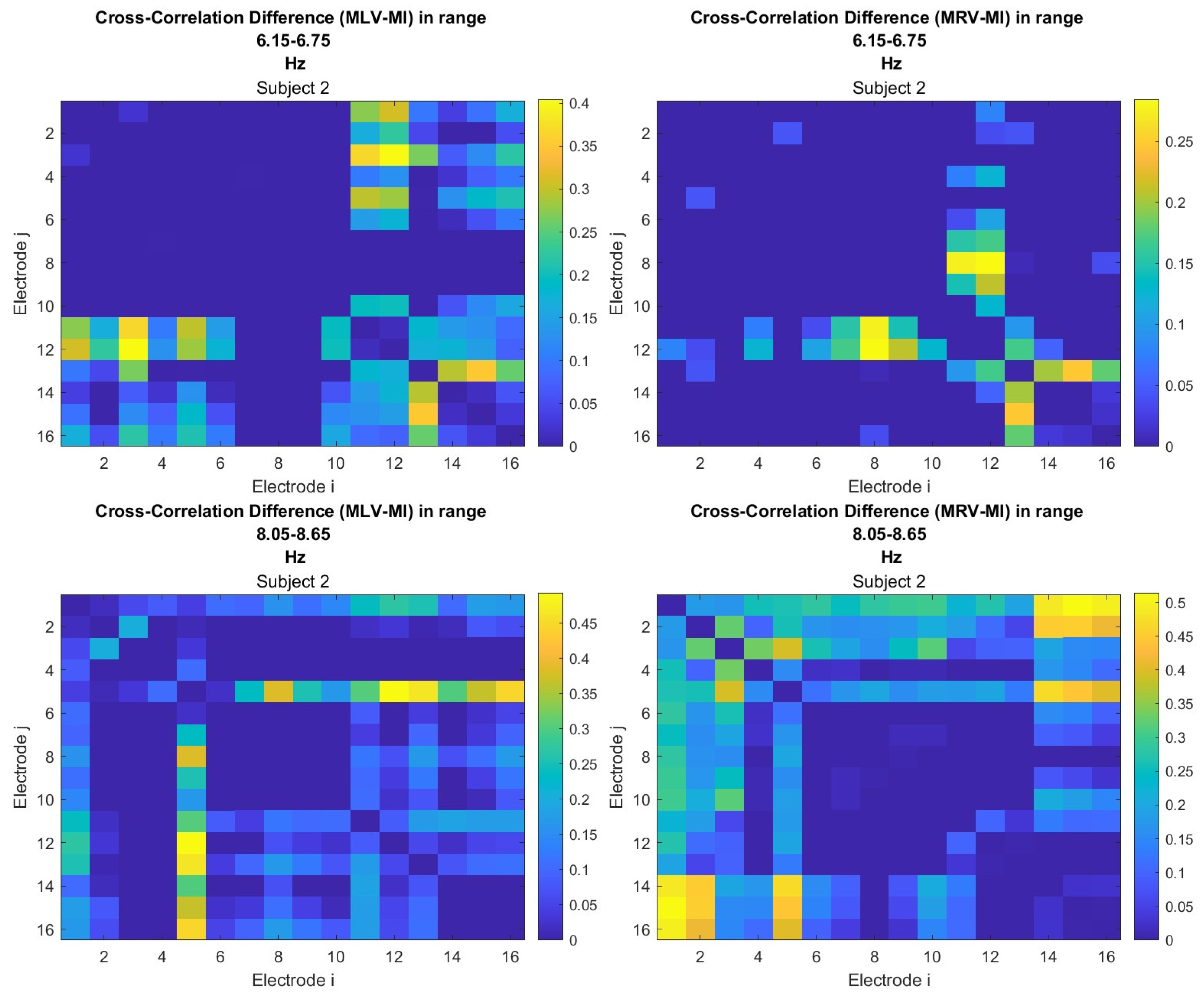
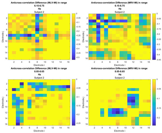
Figure A4.
Decreasing cross-correlation () associated with figurative attention to (left panels) left cube orientation and (right panels) at frequencies (upper raw) and (lower raw) .
Figure A4.
Decreasing cross-correlation () associated with figurative attention to (left panels) left cube orientation and (right panels) at frequencies (upper raw) and (lower raw) .
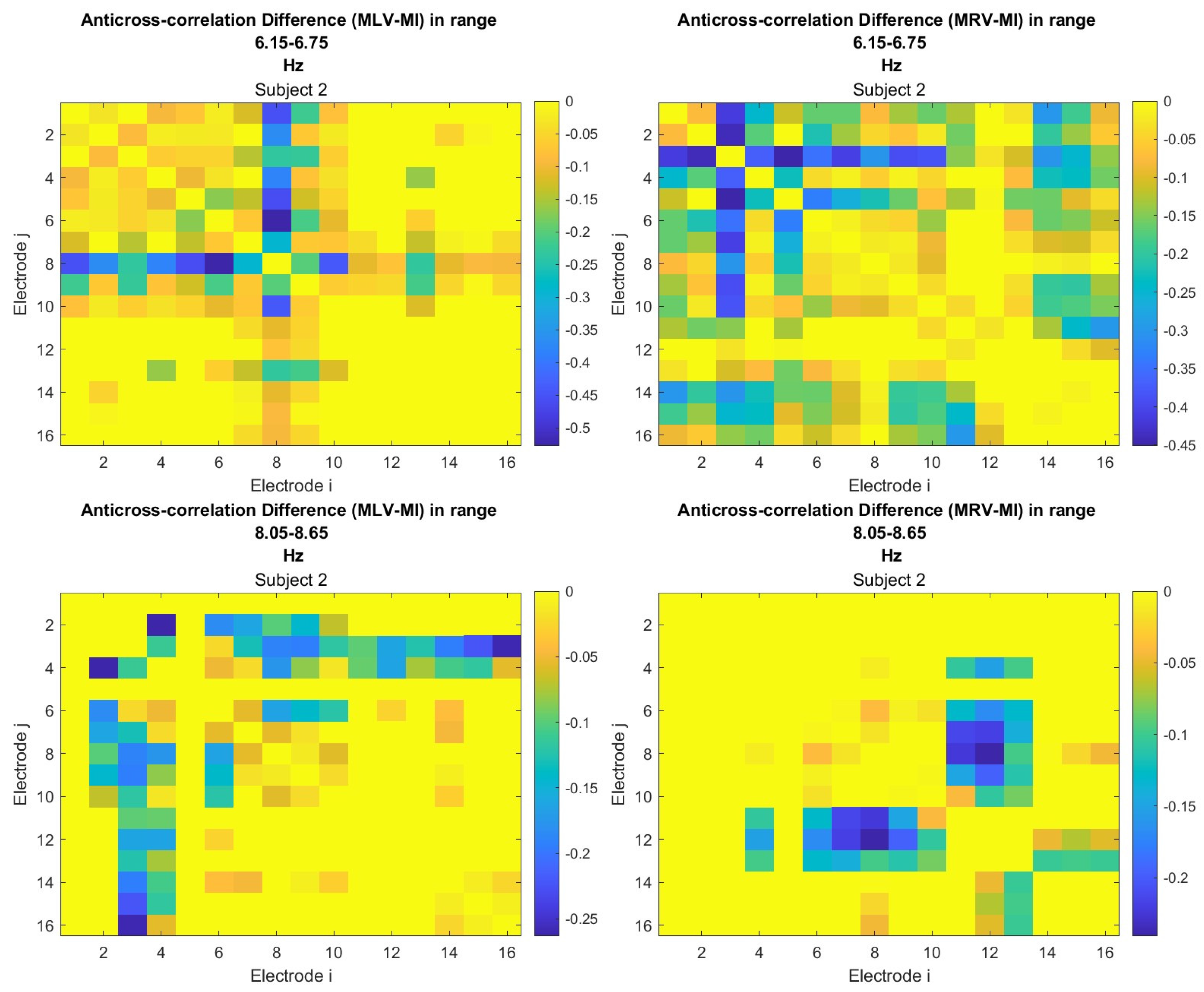

Figure A5.
Increasing mutual information () associated with figurative attention to (left panels) left cube orientation and (right panels) at frequencies (upper raw) and (lower raw) .
Figure A5.
Increasing mutual information () associated with figurative attention to (left panels) left cube orientation and (right panels) at frequencies (upper raw) and (lower raw) .
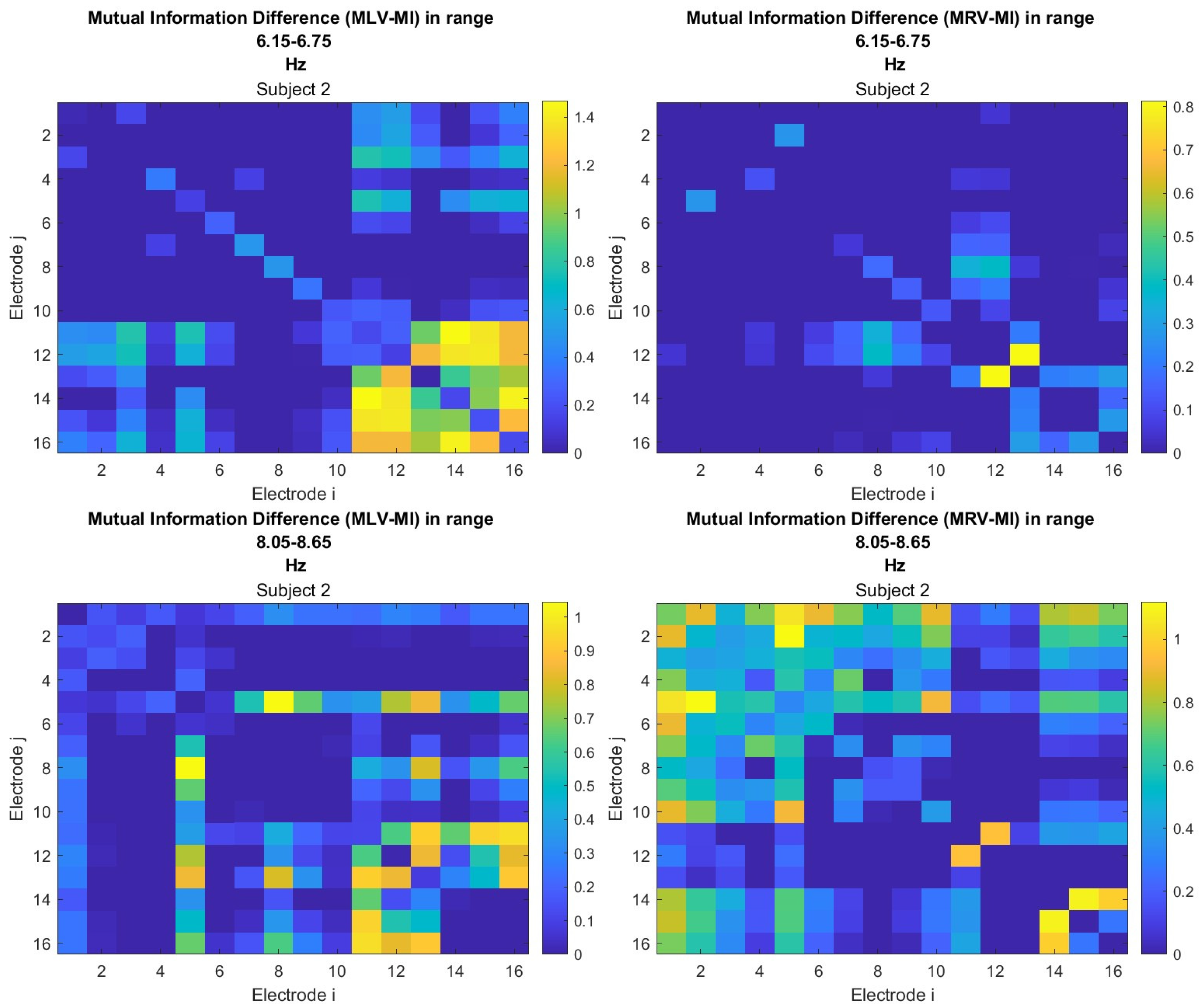
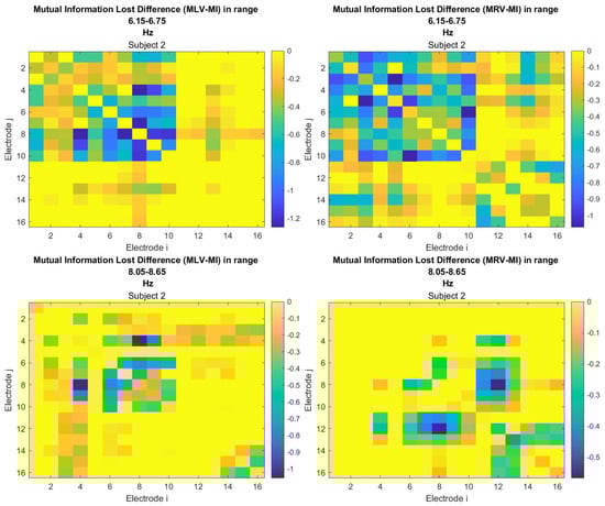
Figure A6.
Decreasing mutual information () associated with figurative attention to (left panels) left cube orientation and (right panels) at frequencies (upper raw) and (lower raw) .
Figure A6.
Decreasing mutual information () associated with figurative attention to (left panels) left cube orientation and (right panels) at frequencies (upper raw) and (lower raw) .
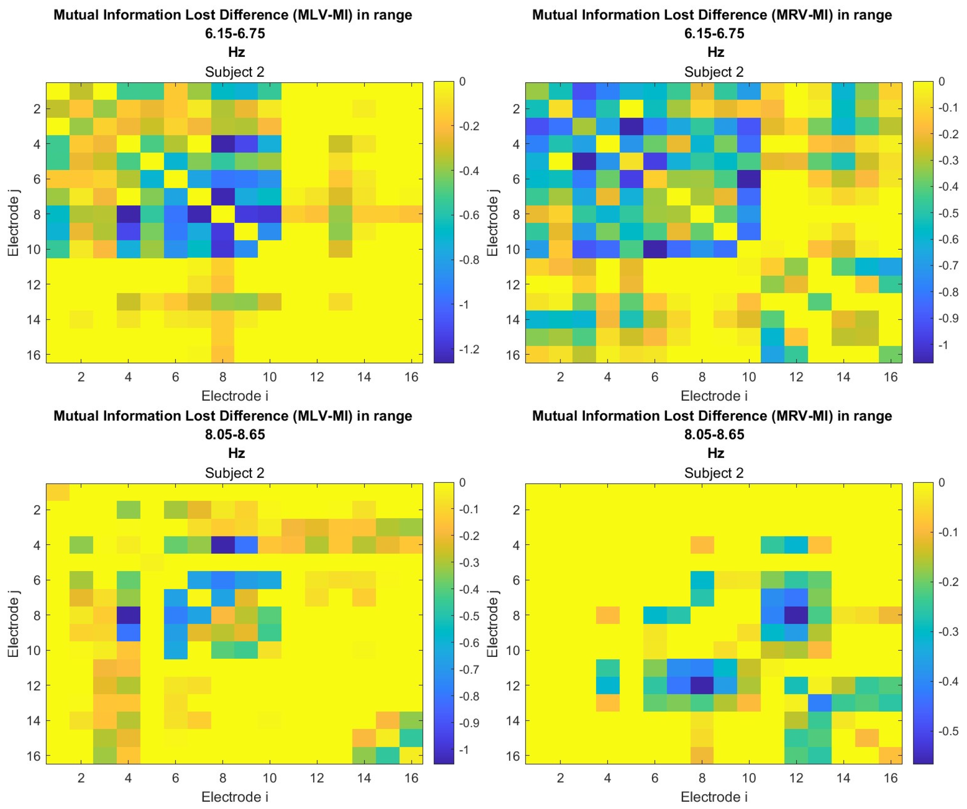
Examining Figure A1, Figure A3 and Figure A5, one can observe a significant increase in connectivity between occipital and frontal regions during attention. Specifically, connectivity is enhanced at when the subject perceives the cube as left-oriented and at when the cube is perceived as right-oriented. This is evident from the warm colors in the lower-left corner of the matrices in the upper-left and lower-right panels.
Appendix C. Probability Measures
The linear probability plots for explored connectivity measures are presented in Figure A7, Figure A8 and Figure A9.
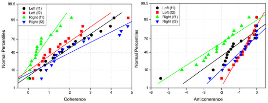
Figure A7.
Normal probability plots of (left) coherence (Lab ) and (right) anticoherence (Lab ) labels. The reference lines have the same colors as percentiles.
Figure A7.
Normal probability plots of (left) coherence (Lab ) and (right) anticoherence (Lab ) labels. The reference lines have the same colors as percentiles.
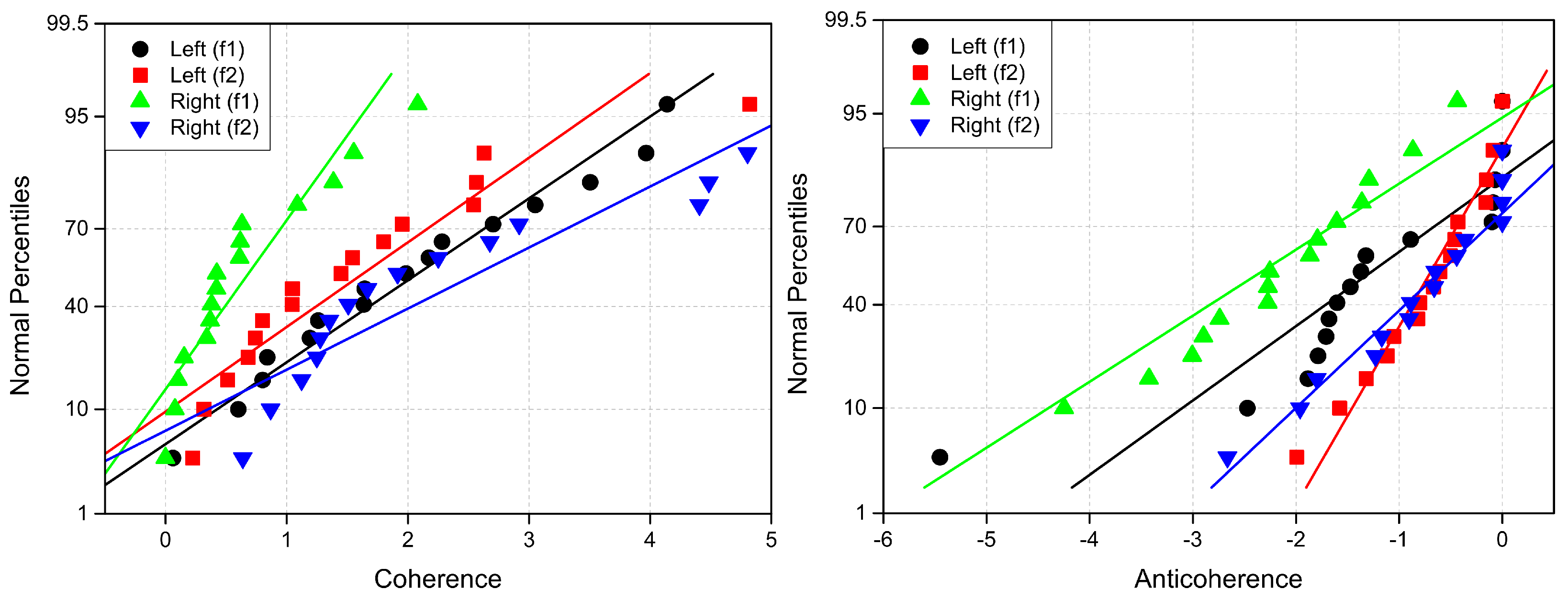
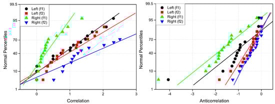
Figure A8.
Normal probability plots of (left) correlation (Lab ) and (right) anticoherence (Lab ) labels. The reference lines have the same colors as percentiles.
Figure A8.
Normal probability plots of (left) correlation (Lab ) and (right) anticoherence (Lab ) labels. The reference lines have the same colors as percentiles.
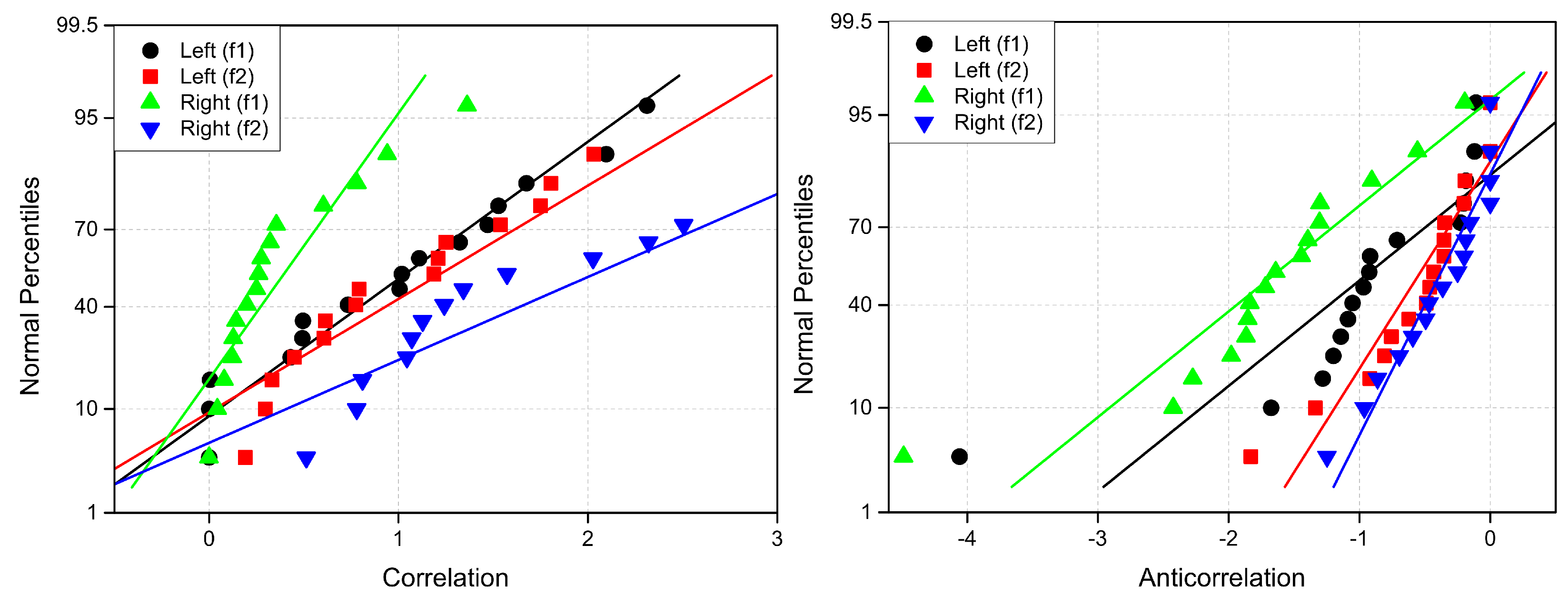
Figure A9.
Normal probability plots of (left) mutual information (Lab ) and (right) information loss (Lab ) labels. The reference lines have the same colors as percentiles.
Figure A9.
Normal probability plots of (left) mutual information (Lab ) and (right) information loss (Lab ) labels. The reference lines have the same colors as percentiles.
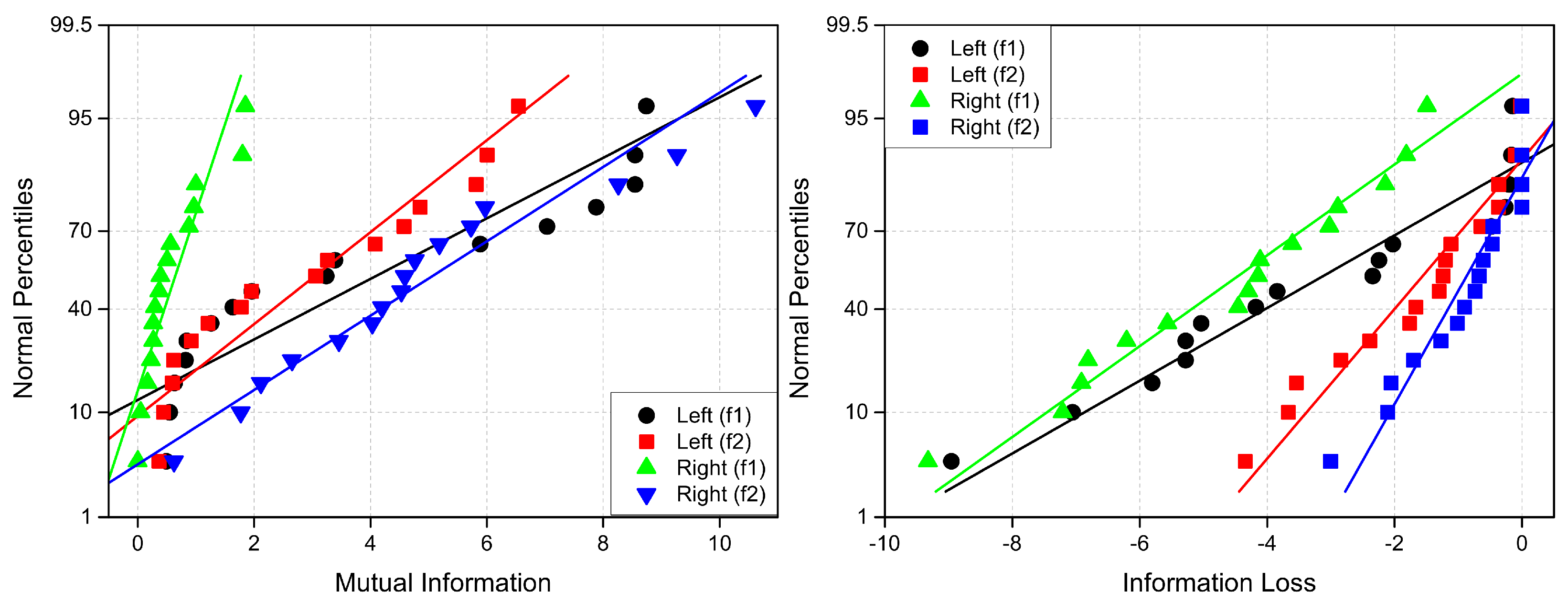
Table A1 presents the means and standard deviations derived from the normal probability plots.
Table A1.
Mean (M), standard deviation (), and threshold () values for the following connectivity measures: coherence (Coh), anticoherence (ACoh), correlation (Corr), anticorrelation (ACorr), mutual information (MInf), and information loss (ILoss).
Table A1.
Mean (M), standard deviation (), and threshold () values for the following connectivity measures: coherence (Coh), anticoherence (ACoh), correlation (Corr), anticorrelation (ACorr), mutual information (MInf), and information loss (ILoss).
| Measure | Left | Left | Right | Right | ||||||||
|---|---|---|---|---|---|---|---|---|---|---|---|---|
| Coh | 1.99 | 1.18 | 3.17 | 1.54 | 1.14 | 2.69 | 0.64 | 0.57 | 1.21 | 2.45 | 1.59 | 4.04 |
| ACoh | 1.31 | 0.55 | 1.48 | 0.55 | ||||||||
| Corr | 0.98 | 0.70 | 1.68 | 1.15 | 0.85 | 2.00 | 0.37 | 0.36 | 0.73 | 1.95 | 1.16 | 3.11 |
| ACorr | 0.92 | 0.47 | 0.91 | 0.37 | ||||||||
| MInf | 3.84 | 3.21 | 7.05 | 2.88 | 2.11 | 4.99 | 0.60 | 0.55 | 1.15 | 4.86 | 2.62 | 7.48 |
| ILoss | 2.67 | 1.30 | 2.14 | 0.86 |
References
- Towle, V.L.; Hunter, J.D.; Edgar, J.C.; Chkhenkeli, S.A.; Castelle, M.C.; Frim, D.M.; Kohrman, M.; Hecox, K. Frequency domain analysis of human subdural recordings. J. Clin. Neurophysiol. 2007, 24, 205–213. [Google Scholar] [CrossRef] [PubMed]
- Hramov, A.E.; Frolov, N.S.; Maksimenko, V.A.; Kurkin, S.A.; Kazantsev, V.B.; Pisarchik, A.N. Functional networks of the brain: From connectivity restoration to dynamic integration. Phys. Uspekhi 2021, 64, 584–616. [Google Scholar]
- Boccaletti, S.; De Lellis, P.; del Genio, C.; Alfaro-Bittner, K.; Criado, R.; Jalan, S.; Romance, M. The structure and dynamics of networks with higher order interactions. Phys. Rep. 2023, 1018, 1–64. [Google Scholar]
- Bullmore, E.; Sporns, O. Complex brain networks: Graph theoretical analysis of structural and functional systems. Nat. Rev. Neurosci. 2009, 10, 186–198. [Google Scholar] [CrossRef]
- Friston, K.J. Functional and effective connectivity: A review. Brain Connect. 2011, 1, 13–36. [Google Scholar]
- Tavor, I.; Jones, O.P.; Mars, R.; Smith, S.; Behrens, T.; Jbabdi, S. Task-free MRI predicts individual differences in brain activity during task performance. Science 2016, 352, 216–220. [Google Scholar]
- Greicius, M. Resting-state functional connectivity in neuropsychiatric disorders. Curr. Opin. Neurol. 2008, 21, 424–430. [Google Scholar] [CrossRef]
- Zhang D, R.M. Disease and the brain’s dark energy. Nat. Rev. Neurol. 2010, 6, 15–28. [Google Scholar]
- Dennis, E.L.; Thompson, P.M. Functional brain connectivity using fMRI in aging and Alzheimer’s disease. Neuropsychol. Rev. 2014, 24, 49–62. [Google Scholar]
- Tomasi, D.; Volkow, N.D. Aging and functional brain networks. Mol. Psychiatry 2012, 17, 549–558. [Google Scholar]
- Sala-Llonch, R.; Bartrés-Faz, D.; Junqué, C. Reorganization of brain networks in aging: A review of functional connectivity studies. Front. Psychol. 2015, 6, 663. [Google Scholar]
- Contreras, J.A.; Goñi, J.; Risacher, S.L.; Sporns, O.; Saykin, A.J. The structural and functional connectome and prediction of risk for cognitive impairment in older adults. Curr. Behav. Neurosci. Rep. 2015, 2, 234–245. [Google Scholar] [PubMed]
- Davison, E.N.; Turner, B.O.; Schlesinger, K.J.; Miller, M.B.; Grafton, S.T.; Bassett, D.S.; Carlson, J.M. Individual differences in dynamic functional brain connectivity across the human lifespan. PLoS Comput. Biol. 2016, 12, e1005178. [Google Scholar]
- Zuo, X.N.; Ehmke, R.; Mennes, M.; Imperati, B.; Castellanos, F.X.; Sporns, O.; Milham, M.P. Network centrality in the human functional connectome. Cereb. Cortex 2012, 22, 1862–1875. [Google Scholar]
- Greene, A.S.; Gao, S.; Scheinost, D.; Constable, R.T. Task-induced brain state manipulation improves prediction of individual traits. Nat. Commun. 2018, 9, 2807. [Google Scholar]
- Gu, S.; Yang, M.; Medaglia, J.D.; Gur, R.C.; Gur, R.E.; Satterthwaite, T.D.; Bassett, D.S. Functional hypergraph uncovers novel covariant structures over neurodevelopment. Hum. Brain Mapp. 2017, 38, 3823–3835. [Google Scholar]
- Xiao, L.; Wang, J.; Kassani, P.H.; Zhang, Y.; Bai, Y.; Stephen, J.M.; Wilson, T.W.; Calhoun, V.D.; Wang, Y.P. Multi-hypergraph learning based brain functional connectivity analysis in fMRI data. IEEE Trans. Med. Imaging 2020, 39, 1746–1758. [Google Scholar]
- Ji, Y.; Zhang, Y.; Shi, H.; Jiao, Z.; Wang, S.H.; Wang, C. Constructing dynamic brain functional networks via hyper-graph manifold regularization for mild cognitive impairment classification. Front. Neurosci. 2021, 15, 669345. [Google Scholar]
- Ji, J.; Ren, Y.; Lei, M. FC–HAT: Hypergraph attention network for functional brain network classification. Inf. Sci. 2022, 608, 1301–1316. [Google Scholar]
- Wu, K.; Song, X.; Chai, L. Graph metrics based brain hypergraph learning in schizophrenia patients. In Proceedings of the 2022 China Automation Congress (CAC), Xiamen, China, 25–27 November 2022; pp. 3251–3256. [Google Scholar]
- Xi, Z.; Liu, T.; Shi, H.; Jiao, Z. Hypergraph representation of multimodal brain networks for patients with end-stage renal disease associated with mild cognitive impairment. Math. Biosci. Eng. 2023, 20, 1882–1902. [Google Scholar]
- Wang, J.; Li, H.; Qu, G.; Cecil, K.M.; Dillman, J.R.; Parikh, N.A.; He, L. Dynamic weighted hypergraph convolutional network for brain functional connectome analysist. Med. Image Anal. 2023, 87, 102828. [Google Scholar] [CrossRef] [PubMed]
- Niua, J.; Dua, Y. Applications of hypergraph-based methods in classifying and subtyping psychiatric disorders: A survey. Radiol. Sci. 2023, 2, 83–95. [Google Scholar] [CrossRef]
- Yang, J.; Hu, M.; Hu, Y.; Zhang, Z.; Zhong, J. Diagnosis of autism spectrum disorder (ASD) using recursive feature elimination-graph neural network (RFE-GNN) and phenotypic feature extractor (PFE). Sensors 2023, 23, 9647. [Google Scholar] [CrossRef] [PubMed]
- Hao, X.; Li, J.; Ma, M.; Qin, J.; Zhang, D.; Liu, F.; for Alzheimer’s Disease Neuroimaging Initiative. Hypergraph convolutional network for longitudinal data analysis in Alzheimer’s disease. Comput. Biol. Med. 2024, 168, 107765. [Google Scholar] [CrossRef]
- Gao, X.; Zhu, Y.; Yang, Y.; Zhang, F.; Zhou, F.; Tian, X.; Xu, K.; Chen, Y. A seizure detection method based on hypergraph features and machine learning. Biomed. Signal Process. Control 2022, 77, 103769. [Google Scholar] [CrossRef]
- Li, M.; Qiu, M.; Zhu, L.; Kong, W. Feature hypergraph representation learning on spatial-temporal correlations for EEG emotion recognition. Cogn. Neurodyn. 2023, 17, 1271–1281. [Google Scholar] [CrossRef]
- Zhu, L.; Liu, Y.; Liu, R.; Peng, Y.; Cao, J.; Li, J.; Kong, W. Decoding multi-brain motor imagery from EEG using coupling feature extraction and few-shot learning. IEEE Trans. Neural Syst. Rehabil. Eng. 2023, 31, 4683–4692. [Google Scholar] [CrossRef]
- Liu, M.; Zhang, J.; Yap, P.T.; Shen, D. View-aligned hypergraph learning for Alzheimer’s disease diagnosis with incomplete multi-modality data. Med. Image Anal. 2017, 36, 123–134. [Google Scholar]
- Peña Serrano, N.; Jaimes-Reátegui, R.; Pisarchik, A.N. Hypergraph of functional connectivity based on event-related coherence: Magnetoencephalography data analysis. Appl. Sci. 2024, 14, 2343. [Google Scholar] [CrossRef]
- Bretto, A. Hypergraph Theory: An Introduction; Mathematical Engineering Series; Springer: Cham, Switzerland, 2013.
- Dai, Q.; Gao, Y. Hypergraph Computation; Springer: Singapore, 2023. [Google Scholar]
- Wang, Z.; Liu, J.; Zhong, N.; Qin, Y.; Zhou, H.; Yang, J.; Li, K. A naïve hypergraph model of brain networks. In Brain Informatics. BI 2012. Lecture Notes in Computer Science; Zanzotto, F.M., Tsumoto, S., Taatgen, N., Yao, Y., Eds.; Springer: Berlin/Heidelberg, Germany, 2012; Volume 7670, pp. 119–129. [Google Scholar]
- Caetano e Souza, R.H.; Martins Naves, E.L. Attention detection in virtual environments using EEG signals: A Scoping review. Front. Physiol. 2021, 12, 727840. [Google Scholar]
- Esqueda-Elizondo, J.J.; Juárez-Ramírez, R.; López-Bonilla, O.R.; García-Guerrero, E.E.; Galindo-Aldana, G.M.; Jiménez-Beristáin, L.; Serrano-Trujillo, A.; Tlelo-Cuautle, E.; Inzunza-González, E. Attention measurement of an autism spectrum disorder user using EEG signals: A case study. Math. Comput. Appl. 2022, 27, 21. [Google Scholar] [CrossRef]
- Mateos, D.M.; Krumm, G.; Arán Filippetti, V.; Gutierrez, M. Power spectrum and connectivity analysis in EEG recording during attention and creativity performance in children. NeuroSci 2022, 3, 347–365. [Google Scholar] [CrossRef]
- Al-Nafjan, A.; Aldayel, M. Predict students’ attention in online learning using EEG data. Sustainability 2022, 14, 6553. [Google Scholar] [CrossRef]
- Escalante Puente de la Vega, W.; Imbert Paredes, R.; Villalba Mora, E.; Pisarchik, A.N. Figurative attention: EEG-based assessment using ambiguous stimuli. Prepr. (Res. Sq.). [CrossRef]
- Bowyer, S.M. Coherence a measure of the brain networks: Past and present. Neuropsychiatr. Electrophysiol. 2016, 2, 1. [Google Scholar]
- Chiarion, G.; Sparacino, L.; Antonacci, Y.; Faes, L.; Mesin, L. Connectivity analysis in EEG data: A tutorial review of the state of the art and emerging trends. Bioengineering 2023, 10, 372. [Google Scholar] [CrossRef]
- Jeong, J.; Gore, J.C.; Peterson, B.S. Mutual information analysis of the EEG in patients with Alzheimer’s disease. Clin. Neurophysiol. 2001, 112, 827–835. [Google Scholar] [CrossRef]
- Zien, J.Y.; Schlag, M.D.F.; Chan, P.K. Multilevel spectral hypergraph partitioning with arbitrary vertex sizes. IEEE Trans. Comput.-Aided Des. Integr. 1999, 18, 1389–1399. [Google Scholar]
- Chholak, P.; Maksimenko, V.A.; Hramov, A.E.; Pisarchik, A.N. Voluntary and involuntary attention in bistable visual perception: A MEG study. Front. Hum. Neurosci. 2020, 14, 597895. [Google Scholar] [CrossRef]
- Liu, Y.; Safavi, T.; Dighe, A.; Koutra, D. Graph summarization methods and applications: A survey. ACM Comput. Surv. 2018, 51, 62. [Google Scholar]
- Maccioni, A.; Abadi, D.J. Scalable pattern matching over compressed graphs via dedensification. In Proceedings of the ACM Conference on Knowledge Discovery and Data Mining (KDD’16), San Francisco, CA, USA, 13–17 August 2016; ACM Press: Cambridge, MA, USA, 2016; pp. 1755–1764. [Google Scholar]
- Andrew, C.; Pfurtscheller, G. Event-related coherence as a tool for studying dynamic interaction of brain regions. Electroencephalogr. Clin. Neurophysiol. 1996, 98, 144–148. [Google Scholar] [PubMed]
- Pisarchik, A.; Hramov, A. Coherence resonance in neural networks: Theory and experiments. Phys. Rep. 2023, 1000, 1–57. [Google Scholar]
- Gross, J.; Schmitz, F.; Schnitzler, I.; Kessler, K.; Shapiro, K.; Hommel, B.; Schnitzler, A. Modulation of long-range neural synchrony reflects temporal limitations of visual attention in humans. Proc. Natl. Acad. Sci. USA 2004, 101, 13050–13055. [Google Scholar] [PubMed]
- Guggisberg, A.G.; Honma, S.M.; Findlay, A.M.; Dalal, S.S.; Kirsch, H.E.; Berger, M.S.; Nagarajan, S.S. Mapping functional connectivity in patients with brain lesions. Ann. Neurol. 2008, 63, 193–203. [Google Scholar]
- Belardinelli, P.; Ciancetta, L.; Staudt, M.; Pizzella, V.; Londei, A.; Birbaumer, N.; Romani, G.L.; Braun, C. Cerebro-muscular and cerebro-cerebral coherence in patients with pre- and perinatally acquired unilateral brain lesions. NeuroImage 2007, 37, 1301–1314. [Google Scholar]
- de Pasquale, F.; Della Penna, S.; Snyder, A.Z.; Lewis, C.; Mantini, D.; Marzetti, L.; Belardinelli, P.; Ciancetta, L.; Pizzella, V.; Romani, G.L.; et al. Temporal dynamics of spontaneous MEG activity in brain networks. Proc. Natl. Acad. Sci. USA 2010, 107, 6040–6045. [Google Scholar] [CrossRef]
- Kim, J.S.; Shin, K.S.; Jung, W.H.; Kim, S.N.; Kwon, J.S.; Chung, C.K. Power spectral aspects of the default mode network in schizophrenia: An MEG study. BMC Neurosci. 2014, 15, 104. [Google Scholar]
- Bowyer, S.M.; Gjini, K.; Zhu, X.; Kim, L.; Moran, J.E.; Rizvi, S.U.; Gumenyuk, N.T.; Tepley, N.; Boutros, N.N. Potential biomarkers of schizophrenia from MEG resting-state functional connectivity networks: Preliminary data. J. Behav. Brain Sci. 2015, 5, 1. [Google Scholar]
- Boutros, N.N.; Galloway, M.P.; Ghosh, S.; Gjini, K.; Bowyer, S.M. Abnormal coherence imaging in panic disorder: A magnetoencephalography investigation. Neuroreport 2013, 24, 487–491. [Google Scholar]
- Chholak, P.; Niso, G.; Maksimenko, V.A.; Kurkin, S.A.; Frolov, N.S.; Pitsik, E.N.; Hramov, A.E.; Pisarchik, A.N. Visual and kinesthetic modes affect motor imagery classification in untrained subjects. Sci. Rep. 2019, 9, 9838. [Google Scholar]
- Pisarchik, A.N.; Chholak, P.; Hramov, A.E. Brain noise estimation from MEG response to flickering visual stimulation. Chaos Solitons Fractals X 2019, 1, 100005. [Google Scholar] [CrossRef]
- Baldassarre, A.; Lewis, C.M.; Committeri, G.; Snyder, A.Z.; Luca Romani, G.; Corbetta, M. Individual variability in functional connectivity predicts performance of a perceptual task. Proc. Natl. Acad. Sci. USA 2012, 109, 3516–3521. [Google Scholar] [CrossRef] [PubMed]
- Kashyap, R.; Kong, R.; Bhattacharjee, S.; Li, J.; Zhou, J.; Thomas Yeo, B.T. Individual-specific fMRI-Subspaces improve functional connectivity prediction of behavior. NeuroImage 2019, 189, 804–812. [Google Scholar]
- Shannon, C.E.; Weaver, W. The Mathematical Theory of Communication; University of Illinois Press: Urbana, IL, USA, 1949. [Google Scholar]
- Cover, T.M.; Thomas, J.A. Elements of Information Theory; John Wiley & Sons: New York, NY, USA, 1991. [Google Scholar]
- Tadel, F.; Baillet, S.; Mosher, J.C.; Pantazis, D.; Leahy, R.M. Brainstorm: A user-friendly application for MEG/EEG analysis. Comput. Intell. Neurosci. 2011, 2011, 879716. [Google Scholar] [CrossRef]
- GitLab.com. Available online: https://gitlab.com/bci_project/visual_stimulation_codes/datas_eeg (accessed on 10 January 2025).
- Hennighausen, E.; Heil, M.; Rösler, F. A correction method for DC drift artifacts. Electroencephalogr. Clin. Neurophysiol. 1993, 86, 199–204. [Google Scholar] [CrossRef]
- Kim, H.; Luo, J.; Chu, S.; Cannard, C.; Hoffmann, S.; Miyakoshi, M. ICA’s bug: How ghost ICs emerge from effective rank deficiency caused by EEG electrode interpolation and incorrect re-referencing. Front. Signal Process. 2023, 3, 1064138. [Google Scholar] [CrossRef]
- Isoglu-Alkaç, U.; Basar-Eroglu, C.; Ademoglu, A.; Demiralp, T.; Miener, M.; Stadler, M. Alpha activity decreases during the perception of necker cube reversals: An application of wavelet transform. Biol. Cybern. 2000, 82, 313–320. [Google Scholar] [CrossRef]
- Adeli, H.; Zhou, Z.; Dadmehr, N. Analysis of EEG records in an epileptic patient using wavelet transform. J. Neurosci. Methods 2003, 123, 69–87. [Google Scholar] [CrossRef]
- Ghuman, A.S.; McDaniel, J.R.; Martin, A. A wavelet-based method for measuring the oscillatory dynamics of resting-state functional connectivity in MEG. Neuroimage 2011, 56, 69–77. [Google Scholar] [CrossRef]
- Maksimenko, V.A.; Hramov, A.E.; Grubov, V.V.; Nedaivozov, V.O.; Makarov, V.V.; Pisarchik, A.N. Nonlinear effect of biological feedback on brain attentional state. Nonlin. Dyn. 2019, 95, 1923–1939. [Google Scholar] [CrossRef]
- Maksimenko, V.A.; Frolov, N.S.; Hramov, A.E.; Runnova, A.E.; Grubov, V.V.; Kurths, J.; Pisarchik, A.N. Neural interactions in a spatially-distributed cortical network during attentional tasks. Front. Behav. Neurosci. 2019, 13, 220. [Google Scholar] [CrossRef] [PubMed]
- Khramova, M.V.; Kuc, A.K.; Maksimenko, V.A.; Frolov, N.S.; Grubov, V.V.; Kurkin, S.A.; Pisarchik, A.N.; Shusharina, N.N.; Fedorov, A.A.; Hramov, A.E. Monitoring the cortical activity of children and adults during cognitive task completion. Sensors 2021, 21, 6021. [Google Scholar] [CrossRef] [PubMed]
- Fang, Q.; Sang, J.; Xu, C.; Rui, Y. Topic-sensitive influencer mining in interest-based social media networks via hypergraph learning. IEEE Trans. Multimed. 2014, 16, 796–812. [Google Scholar]
- Martinet, L.E.; Kramer, M.; Viles, W.; Perkins, L.; Spencer, E.; Chu, C.J.; Cash, S.S.; Kolaczyk, E.D. Robust dynamic community detection with applications to human brain functional networks. Nat. Commun. 2020, 11, 2785. [Google Scholar] [CrossRef]
- Zhao, Z.; Yang, K.; Guo, J. Link prediction with hypergraphs via network embedding. Appl. Sci. 2023, 13, 523. [Google Scholar] [CrossRef]
- Berge, C. Graphs and Hypergraphs; North-Holland: Amsterdam, The Netherlands, 1976. [Google Scholar]
- Bi, X.A.; Wang, Y.; Luo, S.; Chen, K.; Xing, Z.; Xu, L. Hypergraph structural information aggregation generative adversarial networks for diagnosis and pathogenetic factors identification of Alzheimer’s disease with imaging genetic data. IEEE Trans. Neural Netw. Learn. Syst. 2024, 35, 7420–7434. [Google Scholar]
- Harmony, T.; Fernández, T.; Silva, J.; Bernal, J.; Díaz-Comas, L.; Reyes, A.; Marosi, E.; Rodríguez, M.; Rodríguez, M. EEG delta activity an indicator of attention to internal processing during performance of mental tasks. Int. J. Psychophysiol. 1996, 24, 161–171. [Google Scholar]
- Li, X.; Hu, B.; Zhu, T.; Yan, J.; Zheng, F. Towards affective learning with an EEG feedback approach. In Proceedings of the First ACM International Workshop on Multimedia Technologies for Distance Learning, Beijing, China, 23 October 2009; pp. 33–38. [Google Scholar]
- Zhou, S.; Gao, T. Brain activity recognition method based on attention-based RNN mode. Appl. Sci. 2011, 11, 425. [Google Scholar]
- Fahimi, F.; Goh, W.B.; Lee, T.S.; Guan, C. Neural indexes of attention extracted from EEG correlate with elderly reaction time in response to an attentional task. In Proceedings of the 3rd International Conference on Crowd Science and Engineering, Singapore, 28–31 July 2018; pp. 1–6. [Google Scholar]
- Wan, W.; Cui, X.; Gao, Z.; Gu, Z. Frontal EEG-based multi-level attention states recognition using dynamical complexity and extreme gradient boosting. Int. J. Psychophysiol. 2021, 15, 673955. [Google Scholar]
- Myrden, A.; Chau, T. A passive EEG-BCI for single-trial detection of changes in mental state. IEEE Trans. Neural Syst. Rehabil. Eng. 2017, 25, 345–356. [Google Scholar]
- Alirezaei, M.; Hajipour Sardouie, S. Detection of human attention using EEG signals. In Proceedings of the 24th Iranian Conference on Biomedical Engineering and 2nd International Iranian Conference on Biomedical Engineering, Tehran, Iran, 30 November–1 December 2017; pp. 1–5. [Google Scholar]
- Nuamah, J.K.; Seong, Y. Support vector machine (SVM) classification of cognitive tasks based on electroencephalography (EEG) engagement index. Brain-Comput. Interfaces 2018, 5, 1–12. [Google Scholar]
- Aci, c.I.; Kaya, M.; Mishchenko, Y. Distinguishing mental attention states of humans via an EEG-based passive BCI using machine learning methods. Expert Syst. Appl. 2019, 134, 153–166. [Google Scholar] [CrossRef]
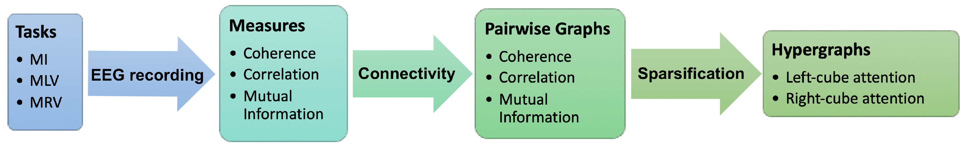
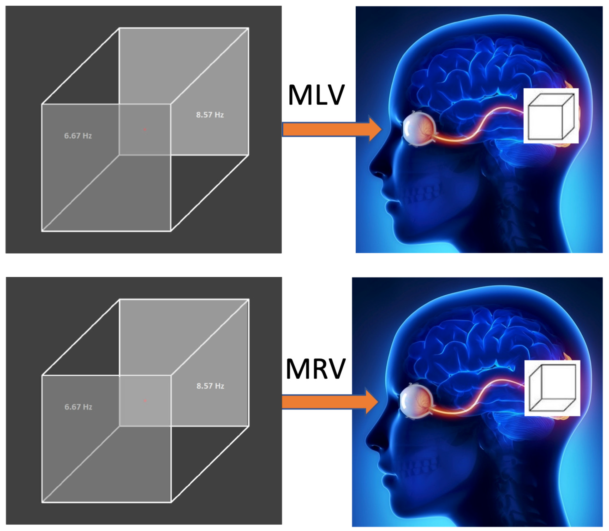
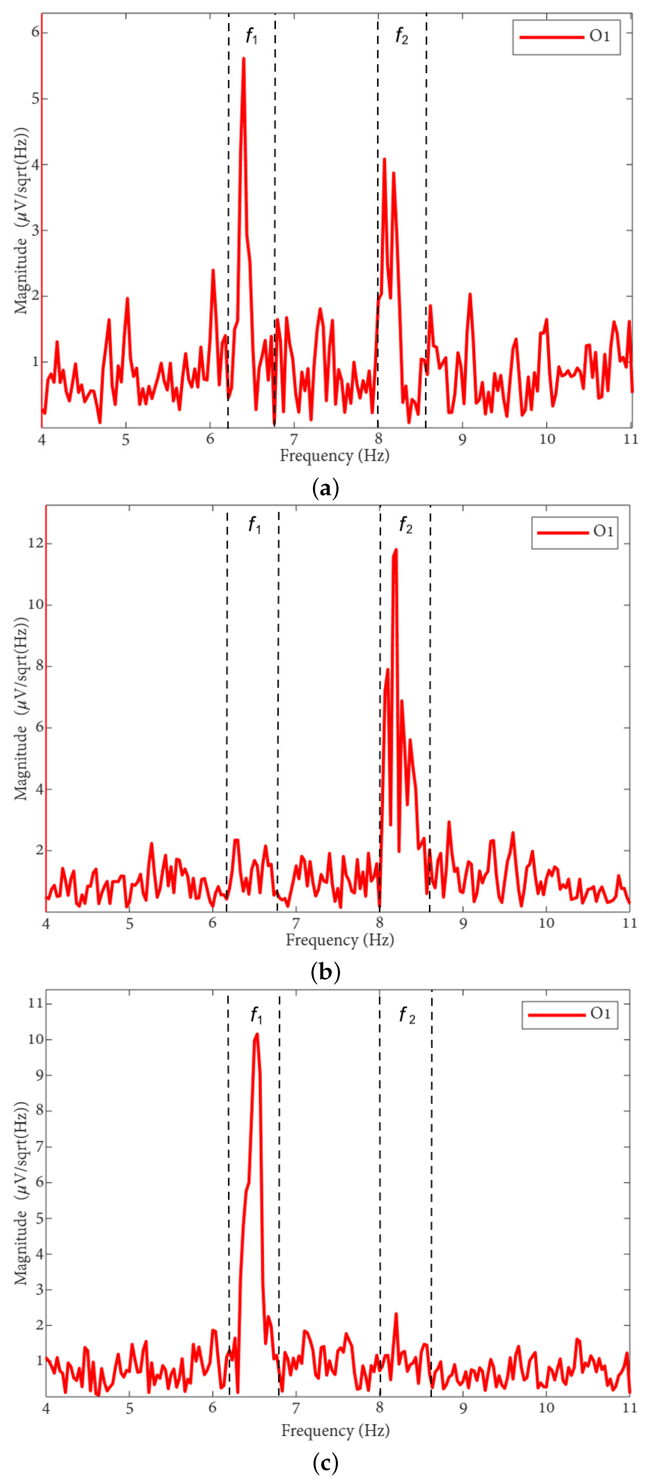
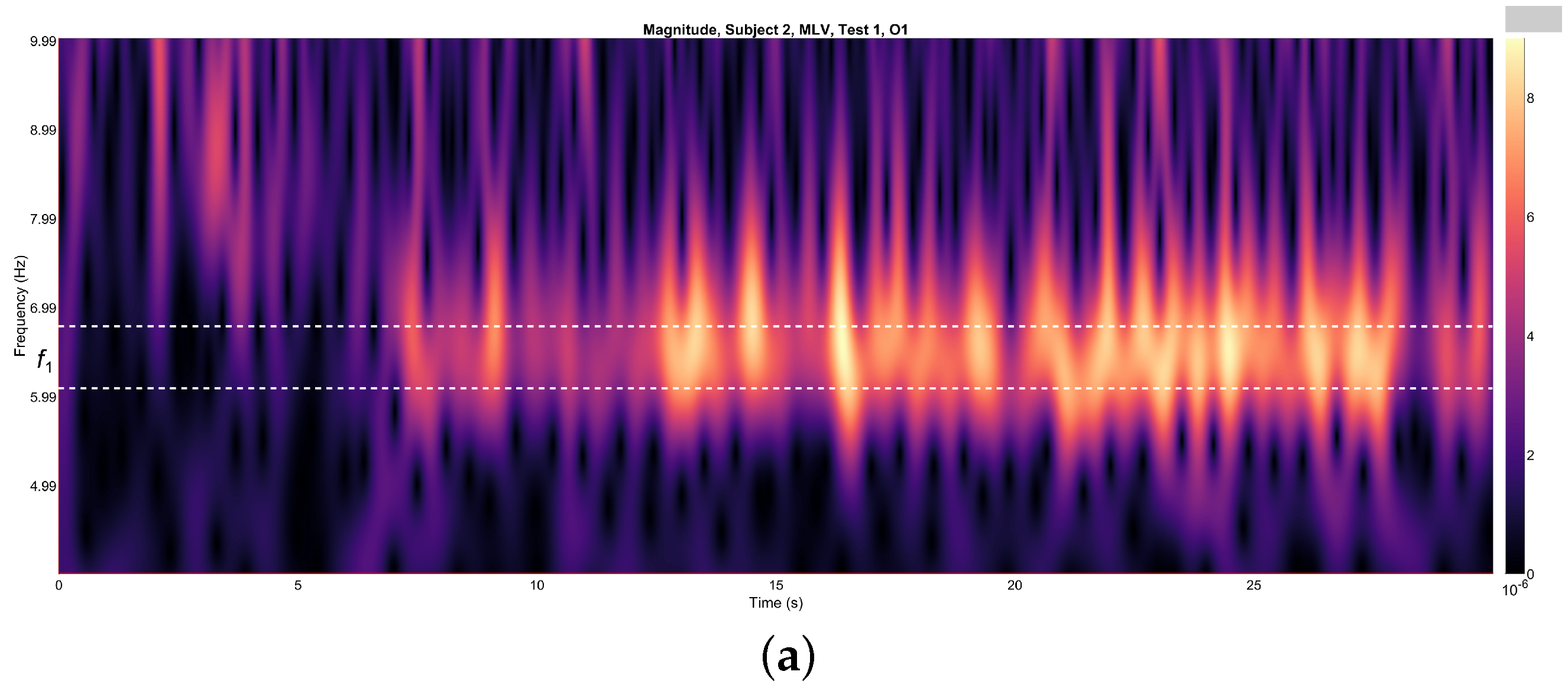

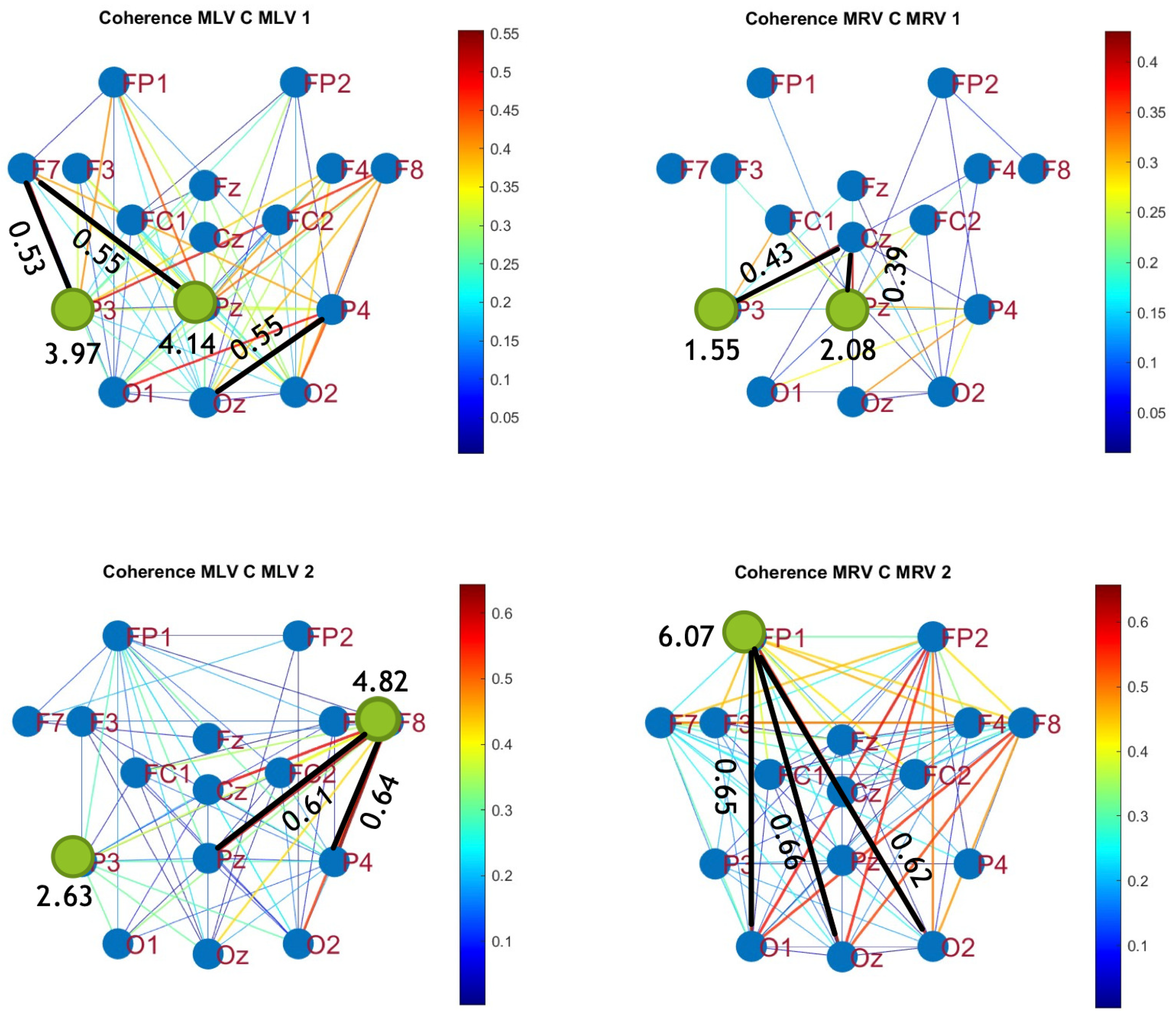
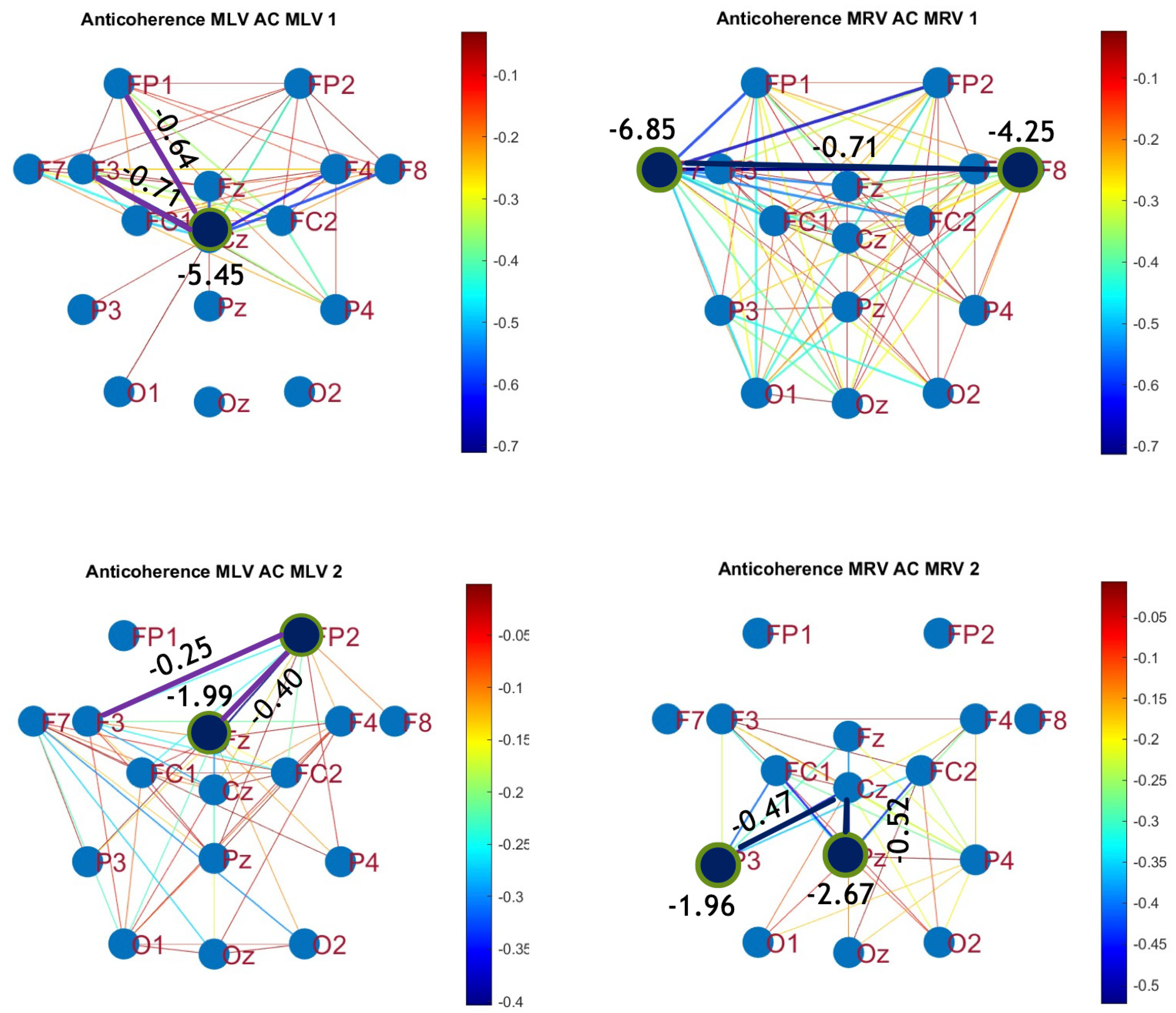
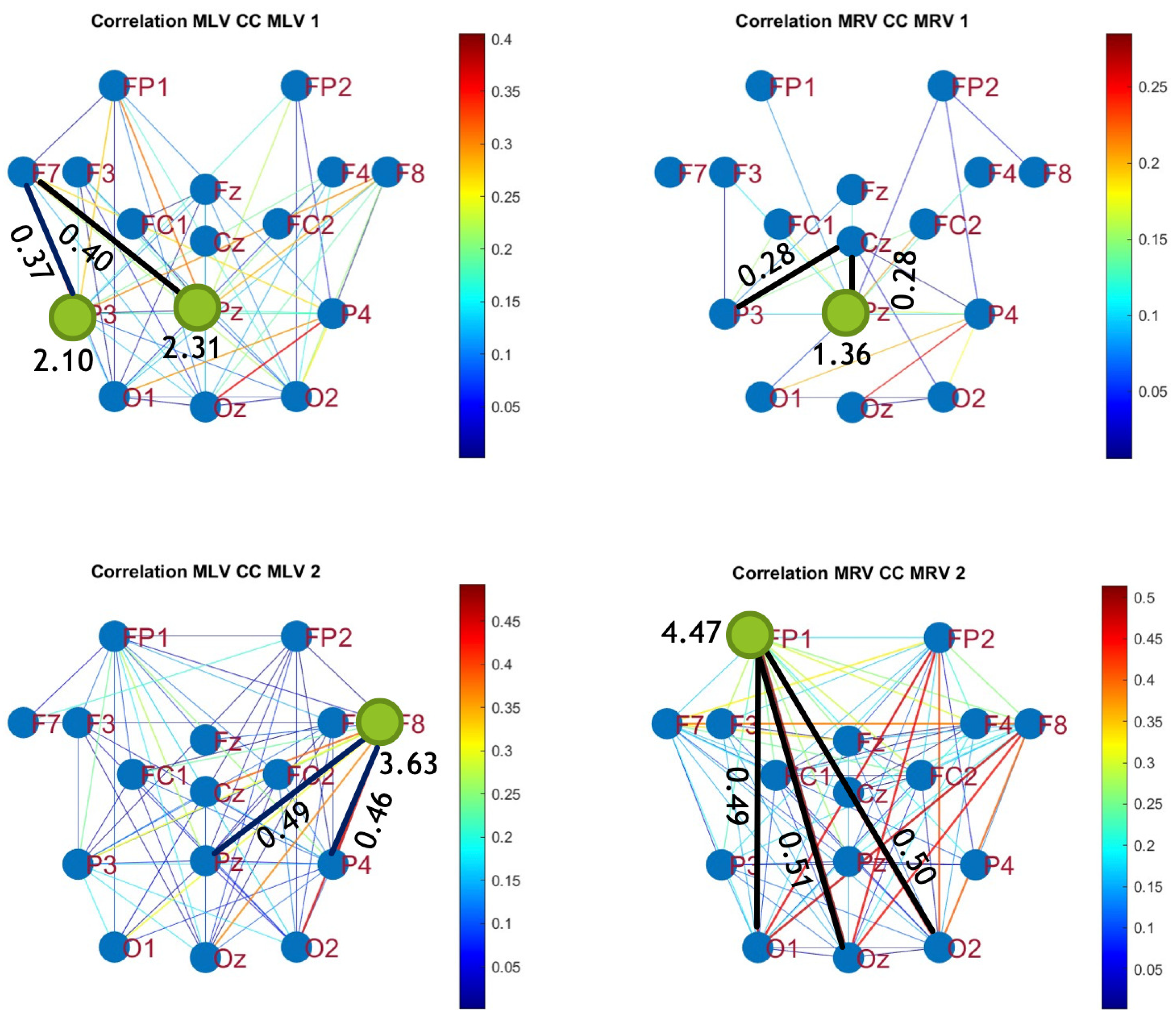
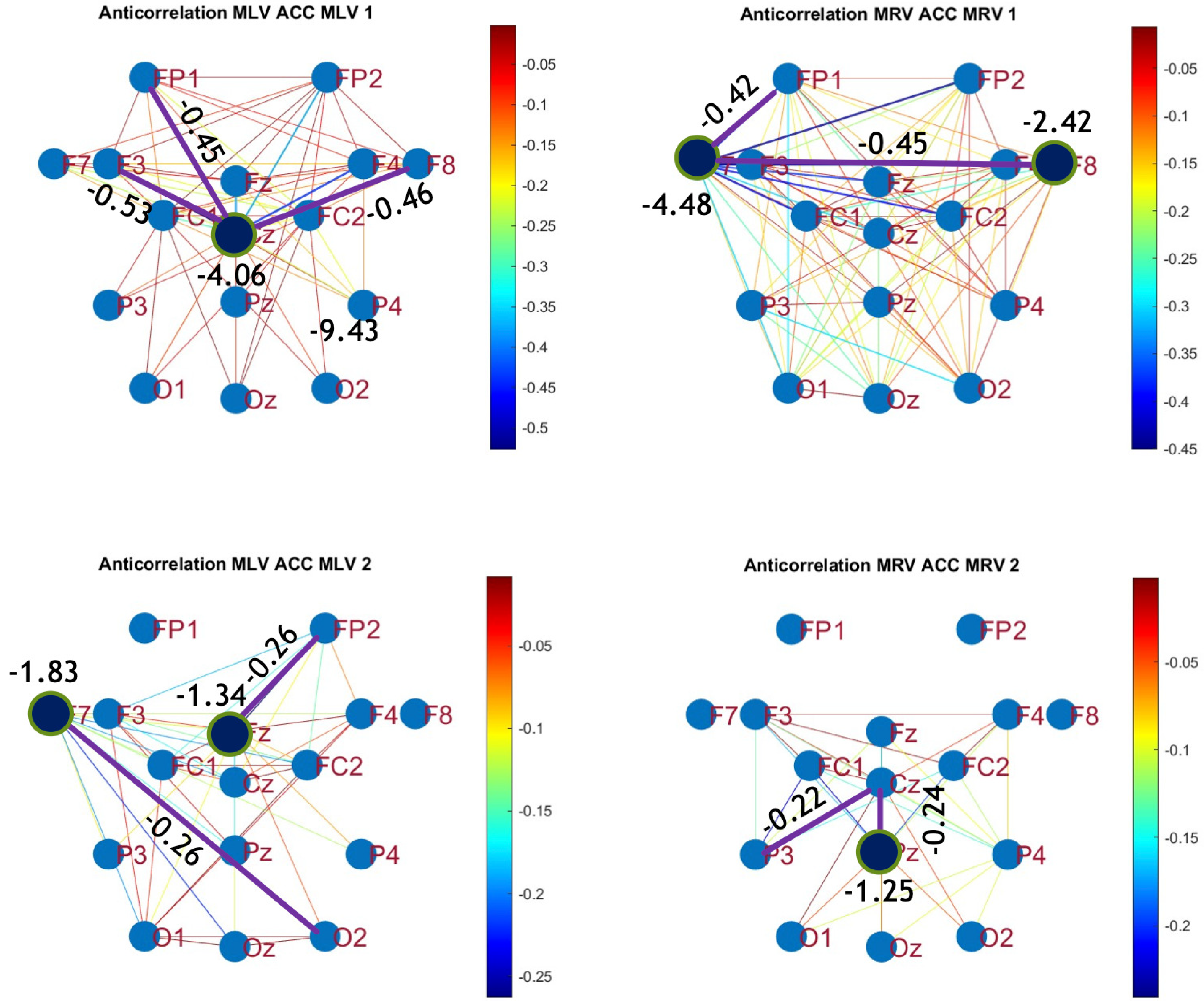

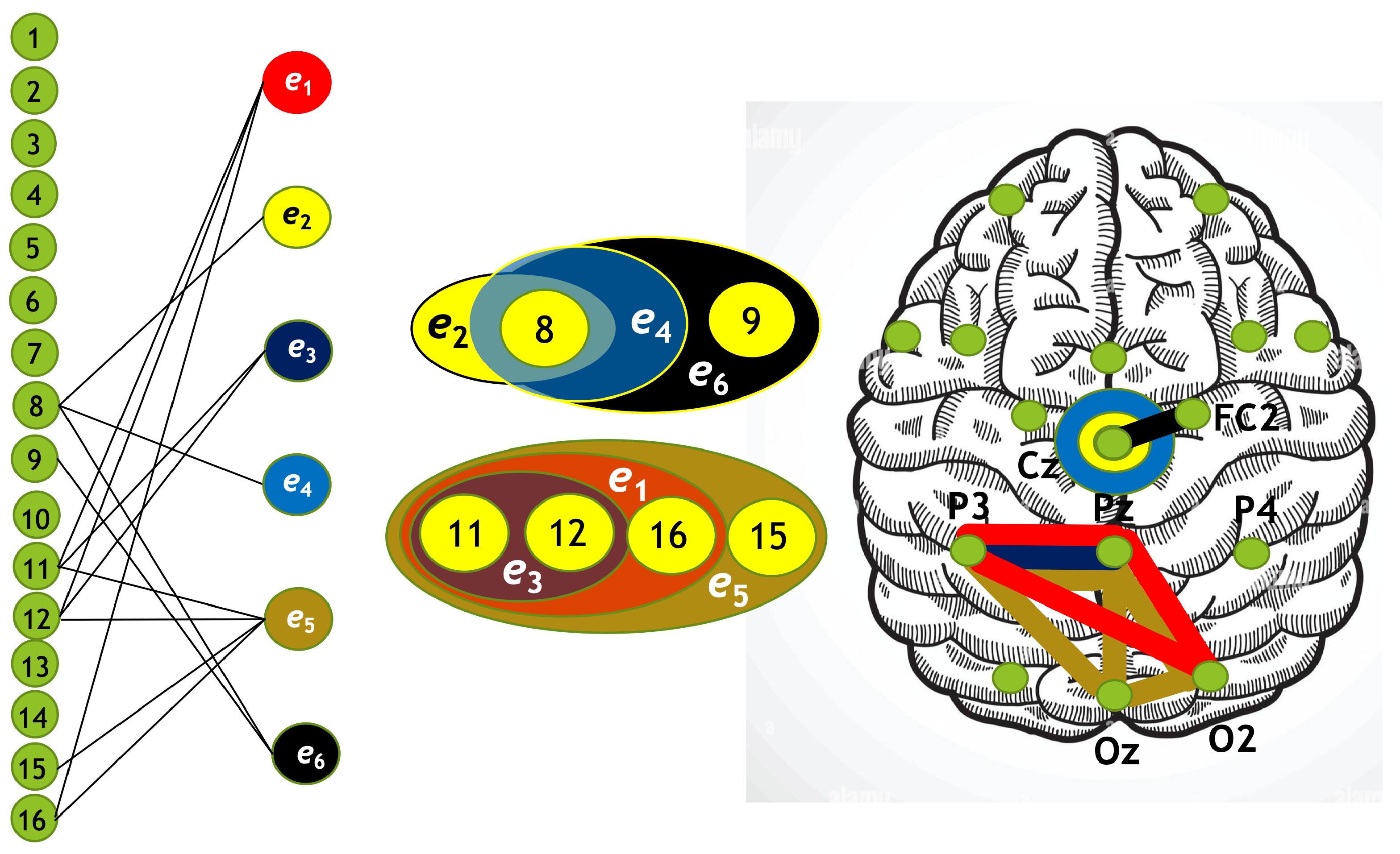
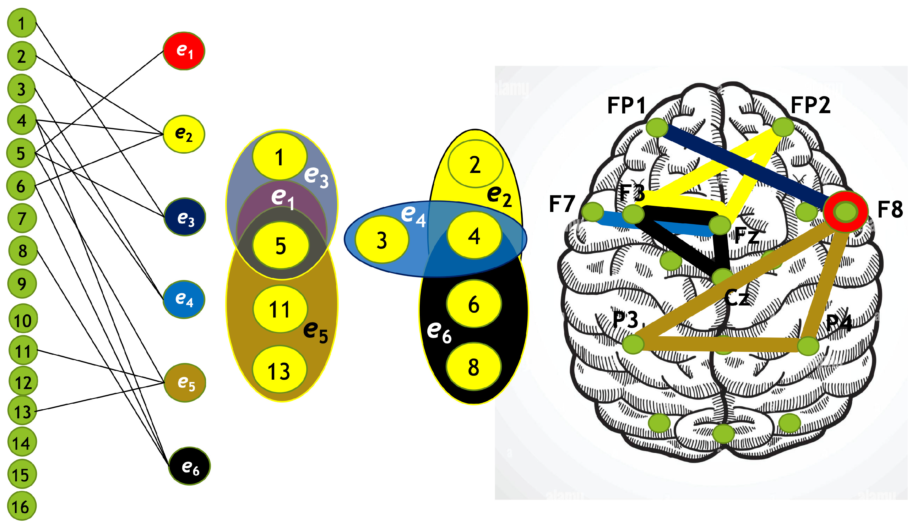
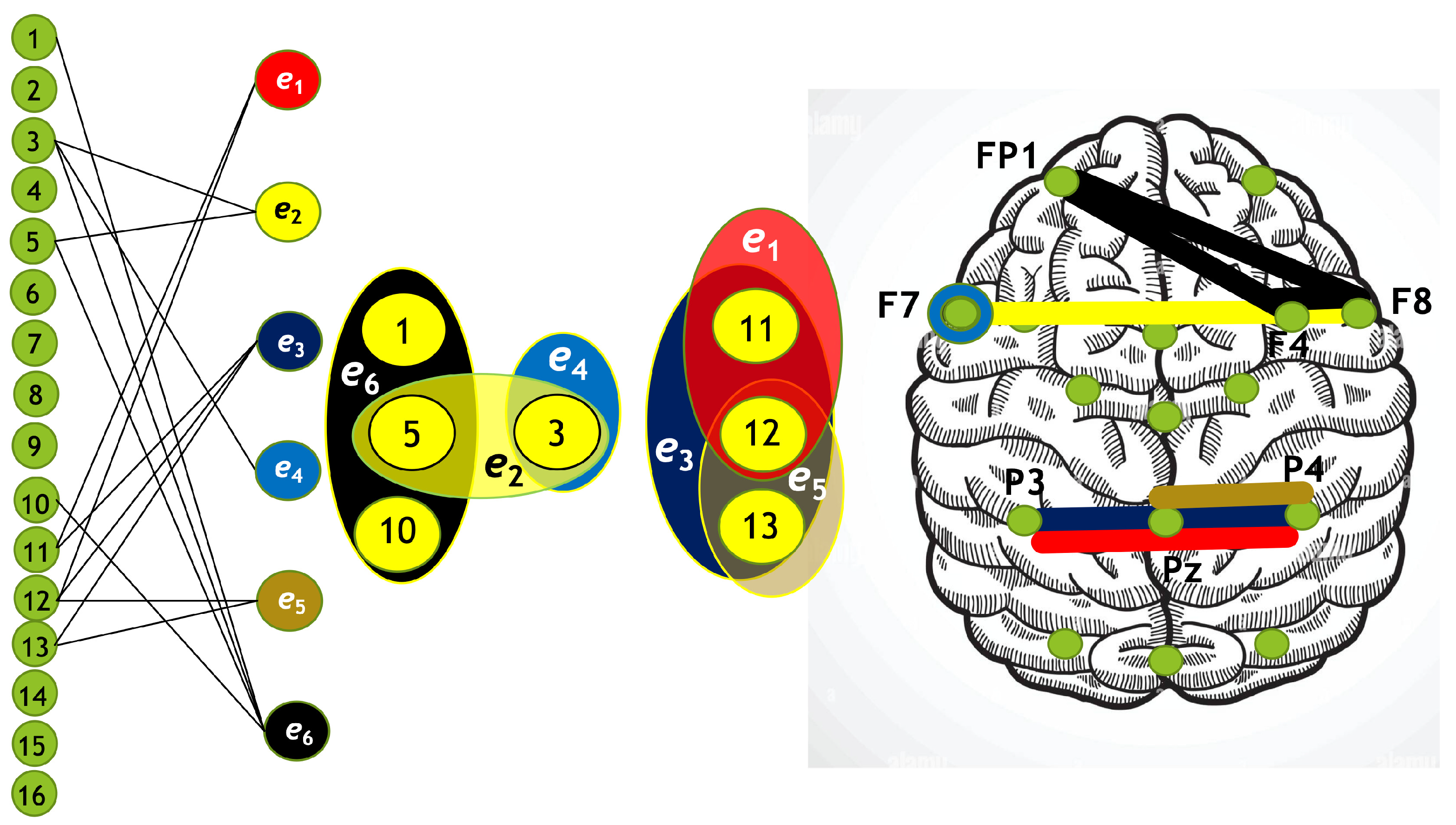

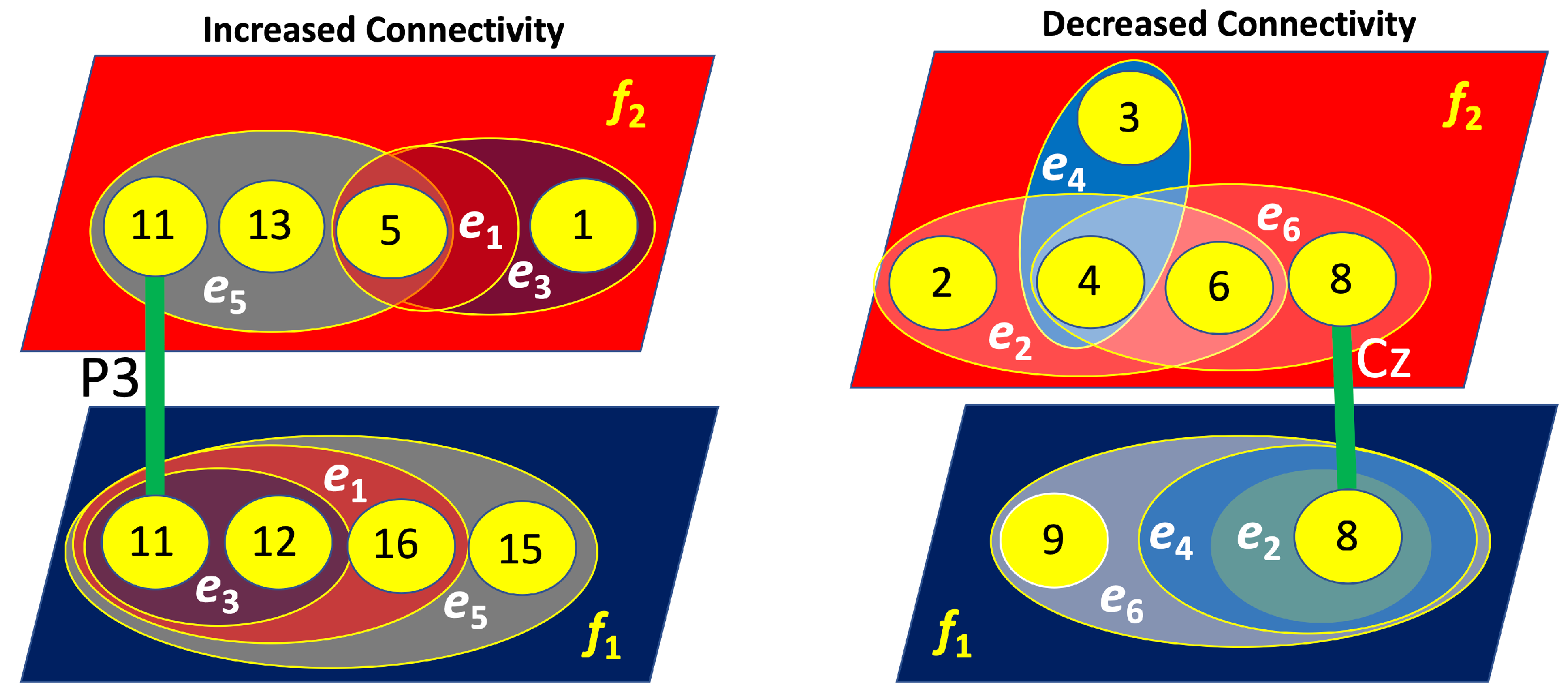
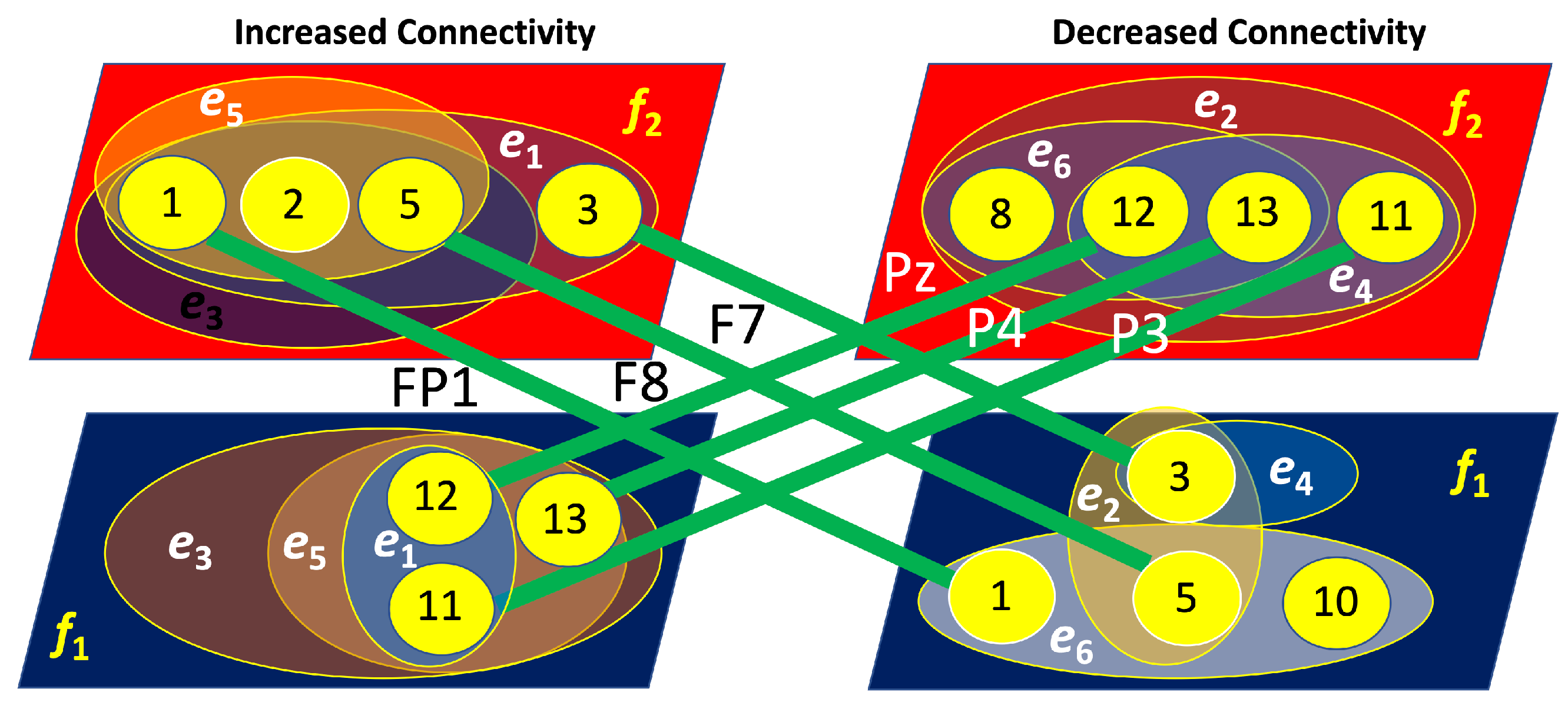
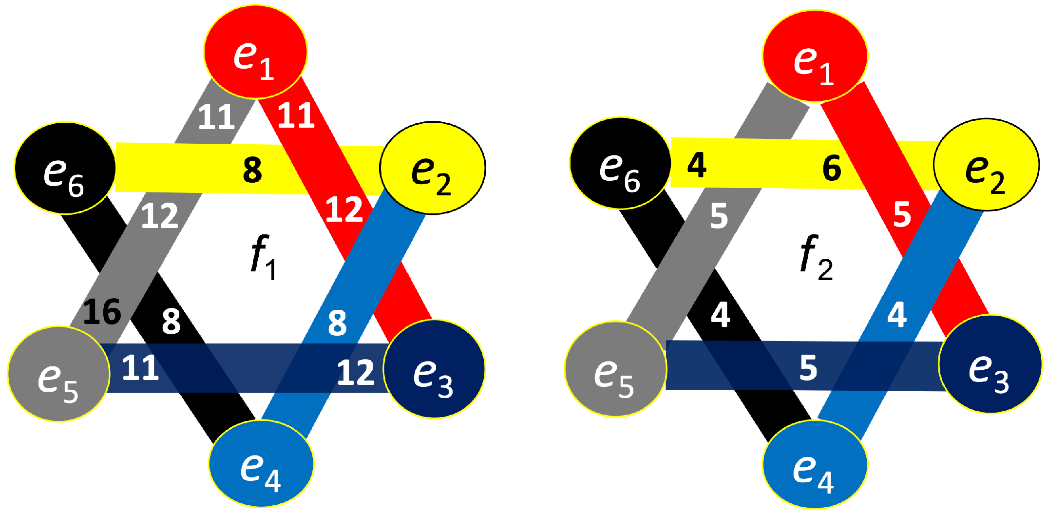
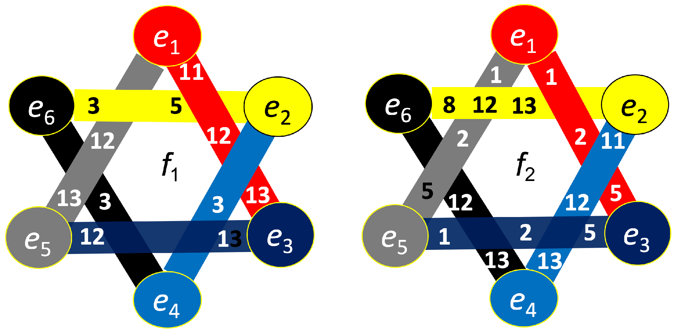
Disclaimer/Publisher’s Note: The statements, opinions and data contained in all publications are solely those of the individual author(s) and contributor(s) and not of MDPI and/or the editor(s). MDPI and/or the editor(s) disclaim responsibility for any injury to people or property resulting from any ideas, methods, instructions or products referred to in the content. |
© 2025 by the authors. Licensee MDPI, Basel, Switzerland. This article is an open access article distributed under the terms and conditions of the Creative Commons Attribution (CC BY) license (https://creativecommons.org/licenses/by/4.0/).