Abstract
Splined assemblies ensure precise torque transmission and alignment in mechanical systems. Three-dimensional printing, especially FDM, enables fast production of customized components with complex geometries, reducing material waste and costs. Optimized printing parameters improve dimensional accuracy and performance. Dimensional accuracy is a critical aspect in the additive manufacturing of mechanical components, especially for splined shafts and hubs, where deviations can impact assembly precision and functionality. This study investigates the influence of key FDM 3D printing parameters—layer thickness, infill density, and nominal diameter—on the dimensional deviations of splined components. A full factorial experimental design was implemented, and measurements were conducted using a high-precision coordinate measuring machine (CMM). To optimize dimensional accuracy, artificial neural networks (ANNs) were trained using experimental data, and a genetic algorithm (GA) was employed for multi-objective optimization. Three ANN models were developed to predict dimensional deviations for different parameters, achieving high correlation coefficients (R2 values of 0.961, 0.947, and 0.910). The optimization process resulted in an optimal set of printing conditions that minimize dimensional errors. The findings provide valuable insights into improving precision in FDM-printed splined components, contributing to enhanced design tolerances and manufacturing quality.
1. Introduction
Splined assemblies play a crucial role in mechanical systems by ensuring precise torque transmission and alignment between shafts and hubs, making them essential for applications requiring high-performance, durability, and operational efficiency. The geometric complexity of splined components, such as involute profiles or straight-sided splines, demands high manufacturing precision to maintain proper fit and minimize wear during operation. The utilization of 3D printing technology in the manufacturing of these assemblies offers significant advantages, particularly through fused-deposition modeling (FDM). This additive manufacturing method enables the rapid production of customized splined components with intricate geometries that are difficult to achieve through conventional machining processes. Additionally, 3D printing reduces material waste, production time, and costs associated with small-batch or prototype manufacturing. The ability to optimize printing parameters, such as layer thickness, infill density, and orientation, further enhances the dimensional accuracy and mechanical properties of the printed parts, contributing to the overall quality and performance of splined assemblies.
Additive manufacturing (AM) technology has gained widespread adoption in recent decades due to its flexibility and ability to produce complex geometries with minimal material consumption. Among the various AM techniques, fused-deposition modeling (FDM) is particularly popular for its cost-effectiveness and versatility in processing different types of polymeric materials [1]. However, despite its advantages, achieving perfect dimensional accuracy remains a challenge in FDM. The process is inherently influenced by factors such as shrinkage, layer-by-layer deposition, and thermal effects during printing, leading to dimensional deviations in manufactured parts. Critical process parameters, including layer thickness, infill density, nozzle temperature, and printing speed, directly impact the final quality and precision of the printed components [2].
Ensuring high-quality production in FDM requires systematic validation and control of dimensional accuracy. The use of appropriate measurement techniques enables precise assessment of product quality and dimensional stability, allowing for better control over manufacturing parameters and minimizing variations. However, post-processing adjustments to correct dimensional inaccuracies are often difficult due to inherent distortions and shrinkage in FDM-printed parts. As the adoption of this technology expands, industries are increasingly prioritizing product quality and demanding stricter performance standards. Consequently, maintaining dimensional variations within tight tolerance limits is crucial for ensuring product reliability and reducing rejection rates in manufacturing [3].
Dimensional accuracy plays a key role in the manufacturing of mechanical components, affecting their performance, reliability, and compatibility within complex assemblies. In the case of splined shafts and hubs, deviations can significantly impact gear precision, assembly stability, and the overall durability of parts. Strict control of these variations is essential to meet design tolerances and minimize premature wear of components. Previous studies have shown that the accuracy of 3D-printed parts can be influenced by factors such as part orientation on the build platform, cooling conditions, and post-processing techniques [4]. In splined shafts, dimensional deviations can result in uncontrolled play in assemblies or excessive interference that complicates assembly and affects functionality.
Objectives of the Study
The primary objectives of this study are as follows:
- To analyze the influence of printing parameters on the dimensional accuracy of splined shafts and hubs manufactured using FDM.
- To identify the dominant factors contributing to significant dimensional deviations.
- To evaluate measurement methods for dimensional deviations and validate them through statistical analysis techniques.
This research aims to contribute to a better understanding of the factors affecting dimensional precision in FDM-printed splined components, facilitating improvements in process optimization and quality control.
2. Literature Review
Numerous studies have explored the dimensional accuracy of FDM-printed parts. According to [5], layer thickness has a major influence on precision, with reductions in thickness leading to improved accuracy. Additionally, [6] emphasizes that infill density plays a key role in maintaining dimensional stability, as higher infill percentages help minimize distortions.
A critical aspect highlighted in previous research is the impact of part orientation on dimensional accuracy. Studies by [7] have shown that vertical orientation can result in greater deviations due to the accumulation of layer-by-layer errors. Moreover, findings from [8] suggest that optimizing the extrusion path can significantly reduce dimensional variations, enhancing the overall precision of printed components.
The FDM process involves complex interactions between various parameters, making it challenging to predict output responses accurately using traditional methods. In recent years, researchers have focused on optimizing one or multiple performance responses in the FDM 3D printing process, employing a diverse array of techniques to enhance dimensional and geometric accuracy. Among non-traditional approaches, artificial neural networks (ANNs) and genetic algorithms (GAs) have gained significant popularity in engineering applications, particularly in optimizing manufacturing processes, due to their ability to model complex relationships and enhance process efficiency [9].
Darbar et al. [10] investigated the influence of three key process parameters in the FDM method—layer thickness, raster width, and build orientation—on the mechanical properties of printed parts. They employed the artificial neural network (ANN) technique to predict the compressive and impact strength of the specimens. Their findings demonstrated a strong correlation between experimental results and ANN predictions, validating the reliability of the developed models.
Camposeco-Negrete [11] conducted an experimental study to analyze the impact of processing variables—processing time, energy consumption of the 3D printer, and dimensional accuracy—on FDM-manufactured parts. Using the Taguchi design, the study optimized five key parameters: layer thickness, filling pattern, printing plane, orientation, and part positioning on the build platform. The results revealed that the printing plane was the most influential factor in minimizing energy consumption and reducing processing time.
Anghel et al. [12] employed a hybrid approach combining genetic algorithms (GAs), artificial neural networks (ANNs), and rational functions to determine the optimal set of printing parameters—layer thickness, infill density, and imposed clearance between the shaft and the hole—for optimizing the absolute relative clearance of cylindrical 3D-printed parts. While the study provided valuable insights into dimensional accuracy, aspects related to operational efficiency, such as energy consumption, scrap weight, and surface roughness, were not within its scope.
Sood et al. [13,14,15] analyzed the impact of process parameters on the dimensional accuracy of FDM-printed parts using the grey–Taguchi method and artificial neural networks (ANNs). Their findings indicated that an optimal combination of process parameters—including a layer thickness of 0.254 mm, a part orientation of 0°, a raster angle of 0°, a raster width of 0.4564 mm, and an air gap of 0.008 mm—yields the best accuracy. Additionally, their investigation into mechanical properties identified the raster angle as the most influential factor [16]. To optimize sliding wear and surface finish, they applied response surface methodology, achieving improved results [17].
Equbal et al. investigated the sliding wear performance and dimensional precision of FDM-printed parts using a Taguchi-based artificial neural network (ANN) approach, identifying part orientation as the most influential factor [18]. Similarly, Sahu et al. [19] analyzed the dimensional accuracy of FDM-printed ABS P400 parts using a fuzzy inference system and concluded that part orientation plays a critical role in maintaining precision. This finding was further corroborated by Padhi et al. [20], who employed the Taguchi method and an ANN, reaching similar conclusions regarding the significance of part orientation [21].
Haghighi and Li [22] explored the correlation between dimensional accuracy and processing cost in FDM-manufactured parts. By applying the desirability function, they optimized fabrication parameters to achieve a balance between precision and cost efficiency. Their study revealed that layer thickness, part inclination, and the interaction between these parameters played a crucial role in influencing both dimensional accuracy and overall production costs, emphasizing the need for careful parameter selection in FDM processes.
When a process requires the simultaneous optimization of multiple objective functions, especially when they are conflicting, multi-objective optimization provides a systematic approach to balancing trade-offs and achieving the best possible outcomes. This method enables the identification of optimal parameter combinations that improve overall performance while addressing competing requirements [23]. NSGA-II is one of the most widely used multi-objective optimization algorithms in FDM applications. Asadollahi-Yazdi et al. [24] applied NSGA-II to analyze the effects of layer thickness and part orientation on production time and material usage in the FDM process. Their formulation incorporated surface roughness and tensile strength as constraints to ensure product quality. The optimization process resulted in 18 Pareto-optimal solutions for the two controllable parameters.
Several studies have explored different approaches to optimizing FDM process parameters. Camposeco-Negrete [11] analyzed the impact of process conditions on processing time, energy consumption, and dimensional accuracy using the Taguchi method and the desirability function. The findings identified layer thickness, road width, and printing plane as the most influential factors. Similarly, Mahmood et al. [25] applied the Taguchi method to optimize the dimensional accuracy and tolerance of FDM-printed parts, revealing that layer thickness, infill speed, infill shell spacing multiplier, number of shells, and extruder temperature significantly affected the results. Their study also proposed optimized process parameters to enhance dimensional accuracy and geometric characteristics in FDM manufacturing.
One of the critical challenges in the fused-deposition modeling (FDM) process is the occurrence of warping deformation, which can significantly impact the dimensional accuracy and mechanical properties of printed parts. Various studies have investigated this phenomenon, proposing models to predict and mitigate its effects. For instance, Wang et al. [26] developed a model to analyze prototype warp deformation in the FDM process, highlighting the influence of material properties, thermal gradients, and layer adhesion on the final part geometry. Their findings suggest that optimizing process parameters such as printing temperature, layer thickness, and cooling rates can reduce deformation and improve print quality.
Bahnini et al. [27] investigated the dimensional accuracy of parts manufactured using fused-deposition modeling (FDM), employing a methodology based on analyzing the relationships between process parameters and dimensional deviations of ABS and ULTRAT parts. The authors applied grey relational analysis (GRA) combined with signal-to-noise (S/N) ratio analysis and analysis of variance (ANOVA) to determine the optimal combination of process parameters that minimize dimensional deviations. The results indicated that part orientation and layer thickness had a significant influence on dimensional accuracy, and experimental validation confirmed that selecting the optimal manufacturing parameters can significantly reduce dimensional deviations.
In the case of splined components, the available literature is relatively limited. However, recent studies, such as [28], suggest that dimensional deviations are significantly influenced by factors such as warping and uneven cooling. These effects become more pronounced in parts with complex geometries, including splined shafts.
Various measurement techniques are employed to analyze dimensional deviations, including 3D scanning, optical interferometry, and coordinate measuring machines (CMMs) [29,30,31]. Research conducted by [32] indicates that while CMM measurements offer superior accuracy compared to optical scanning methods, they require significantly more time.
Another key aspect highlighted in the literature is the impact of post-processing on dimensional accuracy. According to [30], thermal treatments and mechanical finishing of printed components can reduce dimensional deviations by up to 30%, emphasizing the importance of integrating such processes into the production of critical parts.
In summary, this literature review demonstrates that the dimensional accuracy of FDM-printed parts is affected by multiple factors. Implementing an optimized printing approach can significantly enhance the precision and quality of the final components.
3. Materials and Methods
3.1. Materials Used
For this study, 3D-printed splined shafts and hubs made from Z-PLA (polylactic acid made by Zortrax from Olsztyn, Poland) filament were used. Z-PLA is well known for its rigidity and dimensional stability. It is widely utilized in additive manufacturing due to its biocompatibility and lower tendency for thermal deformation compared to other materials such as ABS.
3.2. Printing Parameters
The parts were printed using the Zortrax M200 Plus printer, from Zorteax manufacturer Olsztyn, Poland, a device capable of producing fine details with high precision. The selected printing parameters were as follows:
- Layer thickness: 0.09 mm, 0.14 mm, and 0.19 mm.
- Infill density: 20%, 50%, and 80%.
- Nozzle temperature: 210 °C.
- Printing speed: 50 mm/s.
- Build plate temperature: 60 °C.
These values were chosen based on previous studies to assess the impact of each parameter on dimensional accuracy.
3.3. Part Geometry
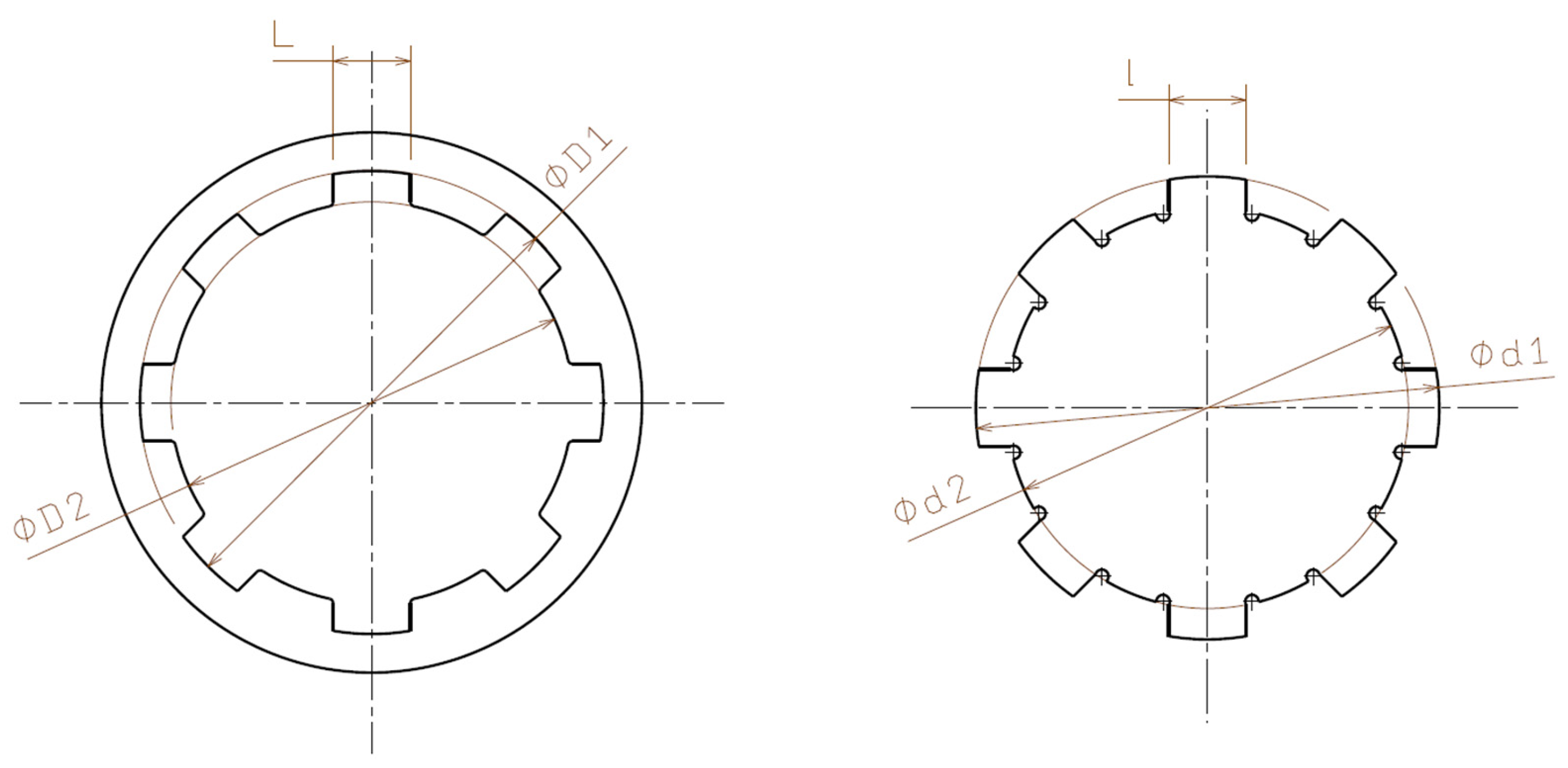
The splined shafts and hubs were designed using Catia V5 R2024 software, Figure 1, and exported in STL format for processing in the Z-Suite v 3.6.0.0 slicing software. The design included specific features to allow precise measurements of diameters and spline widths.
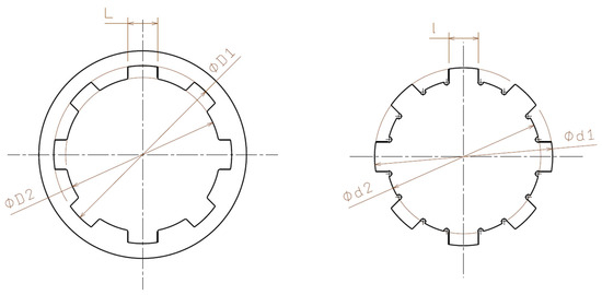
Figure 1.
The splined hub on the left and the splined shaft on the right of the figure.
3.4. Measurement Procedure
The actual dimensions of the printed parts were measured using a Tesa Micro-Hite 3D coordinate measuring machine (CMM) manufactured by Hexagon Manufacturing Intelligence, Renens, Switzerland, with an accuracy of ±0.001 mm. This machine is equipped with an automated probing system, allowing precise dimensional data collection for each part. The associated software enables detailed deviation analysis and the generation of comprehensive reports.
Technical specifications of the measuring machine:
- Model: Tesa Micro-Hite 3D.
- Accuracy: ±0.001 mm.
- Measuring range: 400 × 500 × 450 mm.
- Probing method: Tactile system with an interchangeable probe head.
- Software used: TESA Reflex v.2022, Renens, Switzerland and TESA Power-Inspect v.2022, Renens, Switzerland for dimensional analysis.
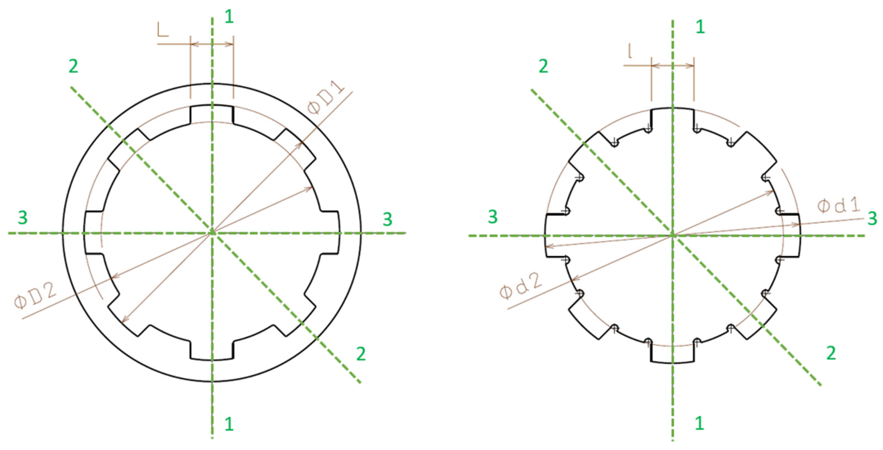
Measurements were conducted along three different directions to evaluate dimensional deviations caused by material shrinkage and variations in the layer deposition process:
- 0°—Axis 1-1: The primary longitudinal direction, corresponding to the alignment of the part on the printing platform.
- 45°—Axis 2-2: A diagonal direction, used to identify irregular shrinkage variations.
- 90°—Axis 3-3: A direction perpendicular to the primary longitudinal axis.
These measurement directions were chosen to provide a comprehensive assessment of dimensional deviations, allowing a precise evaluation of errors induced by the 3D printing process, Figure 2. Measurements were performed 24 h after printing to allow material stabilization and to avoid errors caused by the thermal relaxation of the PLA filament.
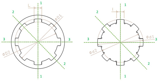
Figure 2.
The measurement scheme.
4. Dimensional Deviations Study
4.1. Experimental Plan
To evaluate the dimensional accuracy of the splined hubs and shafts manufactured using FDM 3D printing, a full factorial experimental design was used. For the study of dimensional accuracy at the nominal diameter Ød1, D1, the key factors considered were as follows:
- Layer thickness (A): 0.09 mm, 0.14 mm, and 0.19 mm;
- Infill density (B): 20%, 50%, and 80%;
- Nominal diameter, Ød1n, ØD1n (C): 48 mm, 54 mm, and 60 mm.
A total of 9 × 3 experiments were conducted (each experiment was repeated three times), as presented in Table 1.

Table 1.
The experimental plan.
4.2. Measurements
Table 2 presents the nominal (n) and measured values (m) for the Ød1, ØD1 diameter of the shaft and hub.
Table 2.
The dataset for the experiment for the Ød1, ØD1 diameter.
Table 3 presents the nominal (n) and measured (m) values for the Ød2, ØD2 diameter of the shaft and hub.
Table 3.
The dataset for the experiment in the case of the Ød2, ØD2 diameter.
Table 4 presents the nominal (n) and measured (m) values for the l, L dimension of the shaft and hub.
Table 4.
The dataset for the experiment in the case of the l, L dimension.
4.3. Data Processing
A multi-objective optimization using a genetic algorithm (GA) was employed to evaluate a given objective function, utilizing a randomly generated population within a predefined range for the input parameters.
Based on the data presented in Table 5, an artificial neural network (ANN) was trained using the input and output datasets structured as follows:
Table 5.
The dataset for the experiment in the case of the absolute relative deviations at Ød1, ØD1.
- Input matrix: (27 × 3).
- Output matrix: (27 × 2).
The Neural Network Toolbox in MATLAB 2024a was used for this purpose.
A multilayer perceptron (MLP) based on a feedforward ANN was implemented to develop the predictive model. The network architecture consists of an input layer, a hidden layer, and an output layer.
The input parameters for the ANN were layer thickness, infill density, and Ø1 n (nominal diameter).
The output parameters were as follows:
- Absolute relative deviation for the shaft (ard Ød1), defined as a ratio in Equation (1).
- Absolute relative deviation for the hole (ard ØD1), defined similarly.
Table 5 presents the absolute relative deviations at Ød1, ØD1 for the shaft and hub.
The connections between inputs, hidden layer, and output were transposed into weights (w) and biases (b), which are considered parameters of the artificial neural network.
The sigmoid tangent function was chosen for the activation of the ANN, and the type of the network was feedforward backpropagation. For the training of the ANN, 70% of the datasets were selected; 15% datasets were used for testing and another 15% for validation.
A value of the correlation coefficient near zero indicates that there is no relationship between the inputs and outputs, and a value very close to 1 indicates a very good correlation.
The already-trained network was used as an objective function by multi-objective optimization using a genetic algorithm, which seeks to minimize the objective function.
The intervals for the three input parameters were [0.09; 20; 48] and [0.19; 80; 60].
The architecture of the network used in this study consisted of the following: three input neurons, corresponding to the input parameters; two output neurons, corresponding to the output parameters; and ten neurons on the hidden layer, empirically chosen, shown in Figure 3.
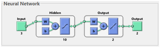
Figure 3.
The neural network architecture.
Using the “Levenberg–Marquardt” backpropagation algorithm, the ANN was trained. The training process is an iterative one. For this study, seven iterations were performed for the training of the network.
At the end of the training process, the “Train Network” window displays the values of the correlation coefficient R2 and the mean squared error (MSE), as shown in Table 6.
Table 6.
The experimental plan.
The results presented in Table 6 indicate a strong correlation between the predicted and actual values across all datasets, as reflected by the high R2 values (above 0.96). The mean squared error (MSE) remains at a very low magnitude, suggesting that the network has achieved a high level of accuracy in training, validation, and testing. Notably, the validation error (MSE = 2.84401 × 10⁻⁷) is slightly higher than the training error (MSE = 2.16272 × 10⁻⁷), which is expected as the model generalizes to unseen data. However, the increase in MSE for the test set (4.87121 × 10⁻⁷) suggests a slight overfitting, meaning the model might perform marginally better on training data than on entirely new inputs. Nonetheless, the overall performance remains strong, indicating a well-trained network with good generalization capabilities.
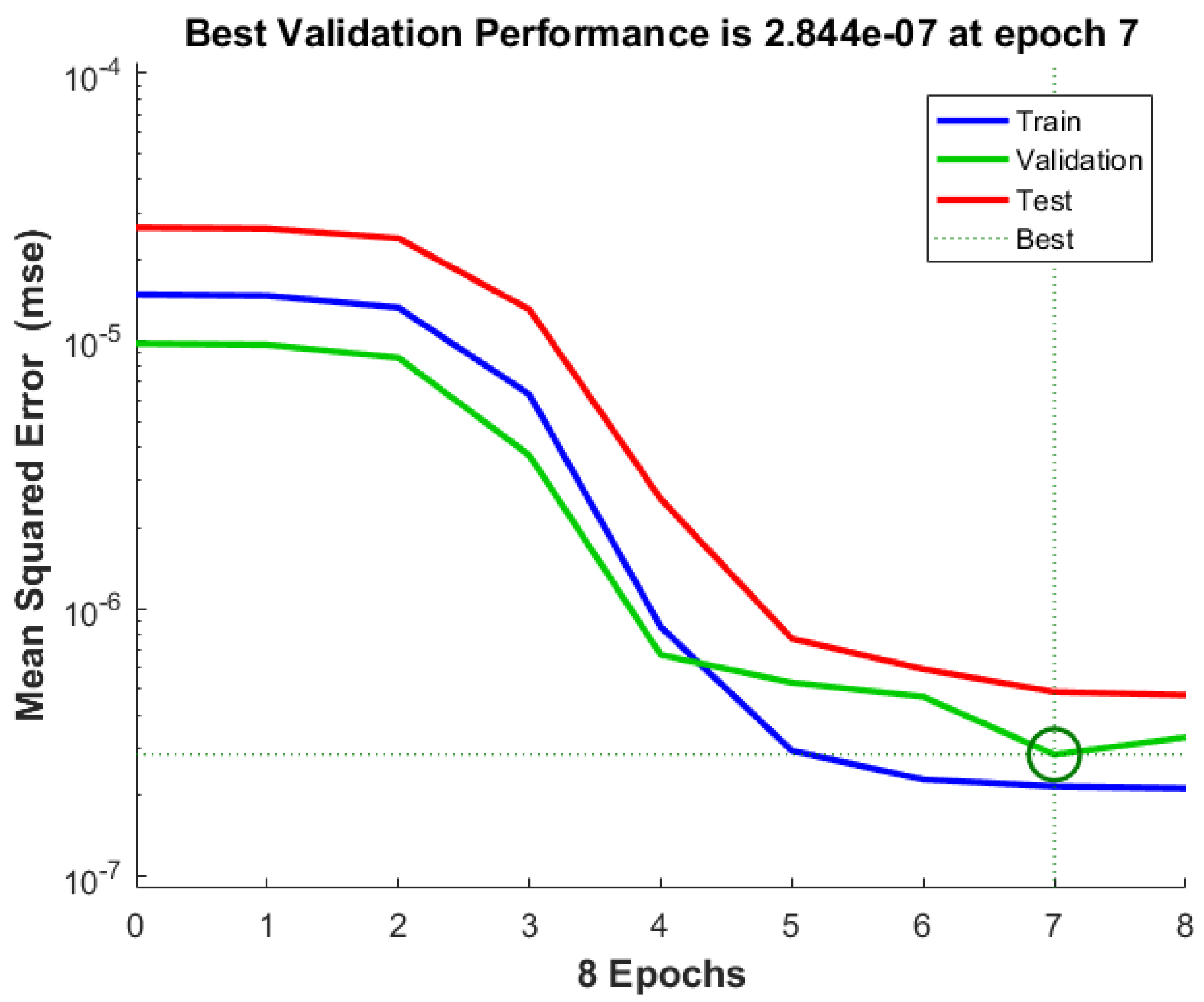
Figure 4 illustrates the learning curve of the neural network by displaying the mean squared error (MSE) for the training, validation, and test datasets over eight epochs. The blue, green, and red curves represent the training, validation, and test errors, respectively. The model achieves its best validation performance at epoch 7, with an MSE of 2.844 × 10⁻⁷, as indicated by the green dotted line and the marked point on the graph.
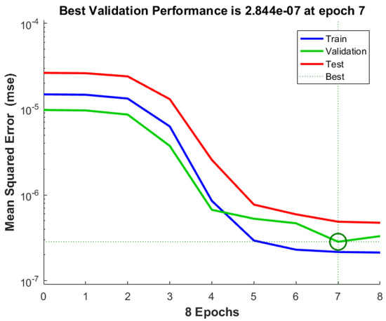
Figure 4.
Training, validation, and test error evolution over epochs.
The downward trend of all three curves suggests that the model is learning effectively, with the errors decreasing as training progresses. However, after epoch 7, the validation and test errors stabilize, while the training error continues to decrease slightly. This behavior suggests that further training might lead to overfitting, where the model becomes too specialized to the training data and loses generalization capability. Therefore, stopping the training at epoch 7 ensures the best trade-off between accuracy and generalization.
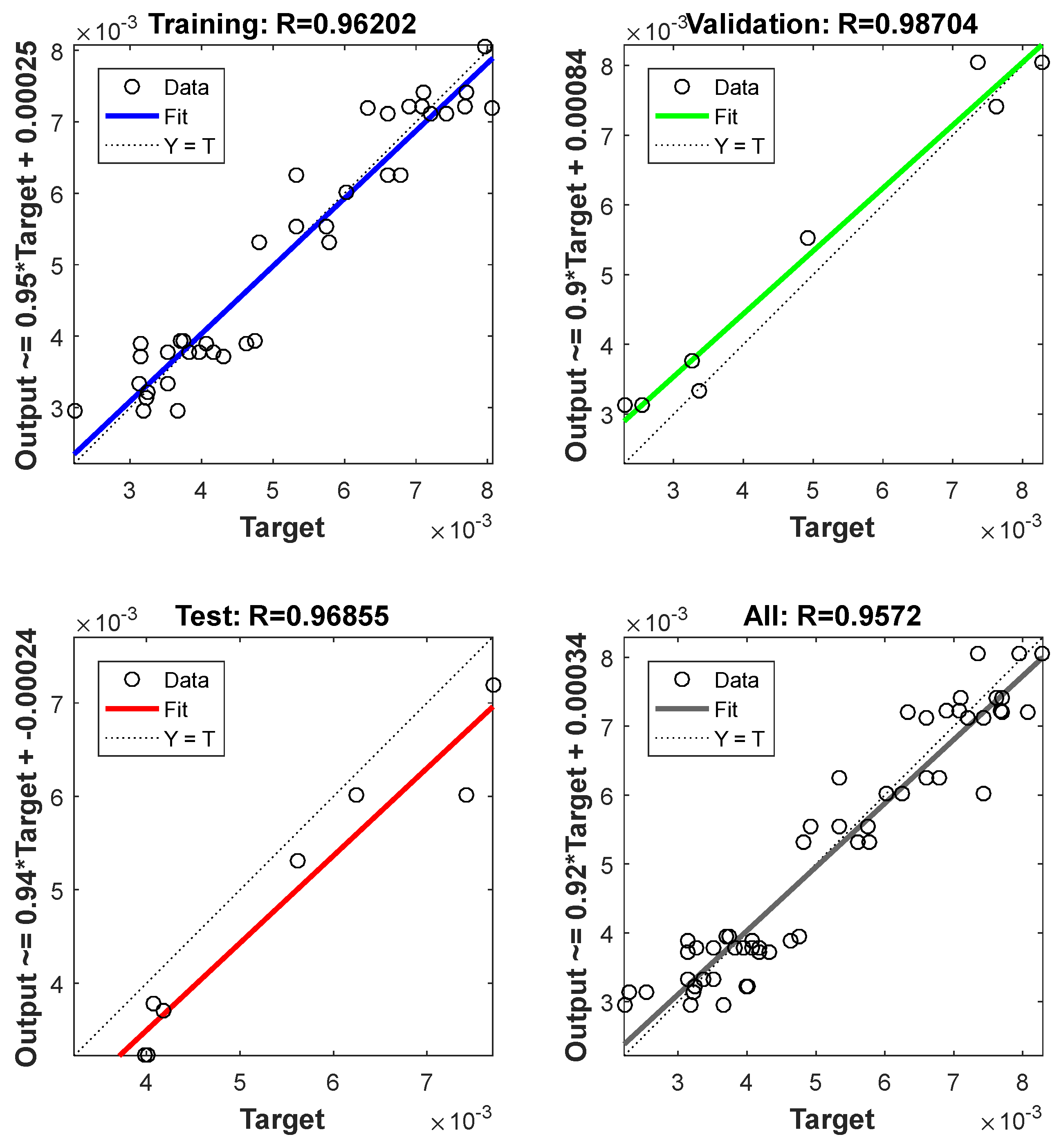
The training process was validated when an overall R2 value (0.957) was obtained. Figure 5 presents the values of R2 for training, testing, validation, and the value of the overall R2.
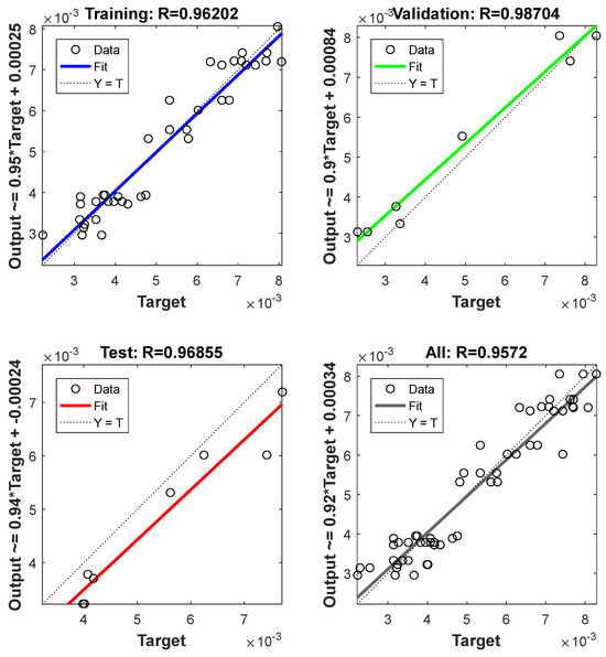
Figure 5.
The values of R2 for training, testing, and validation processes.
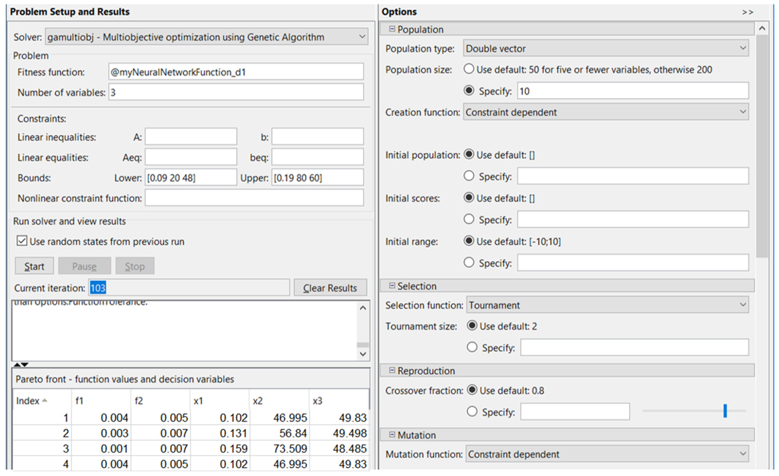
The values of the specific gamultiobj multi-objective optimization using genetic algorithm parameters were the following: population size = 10, crossover, crossover ratio = 0.8, reproduction, and crossover fraction = 0.8.
After 103 iterations, in the case corresponding to diameter Ød1, ØD1, the optimized conditions were obtained, as shown in Figure 6.
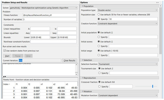
Figure 6.
Optimization using a genetic algorithm for Ød1, ØD1 diameters.
Table 7 presents the absolute relative deviations at Ød2, ØD2 for the shaft and hub.
Table 7.
The dataset for the experiment in the case of the absolute relative deviations at Ød2, ØD2.
In this case, an identical architecture to the first network was used for a second neural network, which was trained, tested, and validated: three input neurons, corresponding to the input parameters; two output neurons, corresponding to the output parameters; and ten neurons on the hidden layer, empirically chosen. For this process, the overall R2 is 0.947.
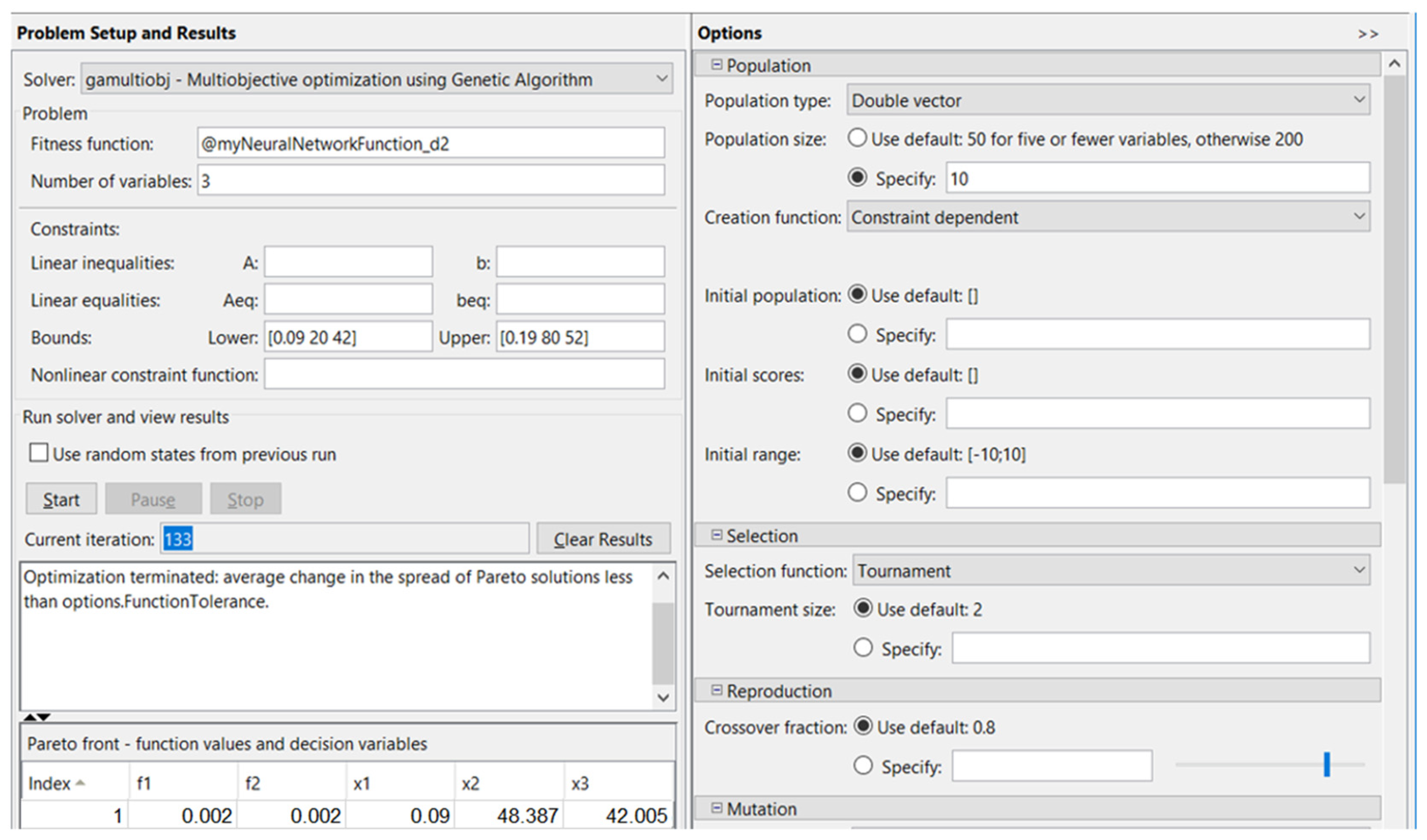
By optimization using the genetic algorithm, after 133 iterations, in the case corresponding to diameter Ød2, ØD2, the optimized conditions were obtained, as shown in Figure 7.
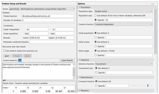
Figure 7.
Optimization using the genetic algorithm for Ød2, ØD2 diameters.
The absolute relative deviations of l, L for both the shaft and the hub are presented in Table 8.
Table 8.
The dataset for the experiment in the case of the absolute relative deviations at l, L.
In this case, a third neural network was trained, tested, and validated. This network has an identical architecture to the other networks: three input neurons, corresponding to the input parameters; two output neurons, corresponding to the output parameters; and ten neurons on the hidden layer, empirically chosen. For this process, the overall R2 is 0.910.
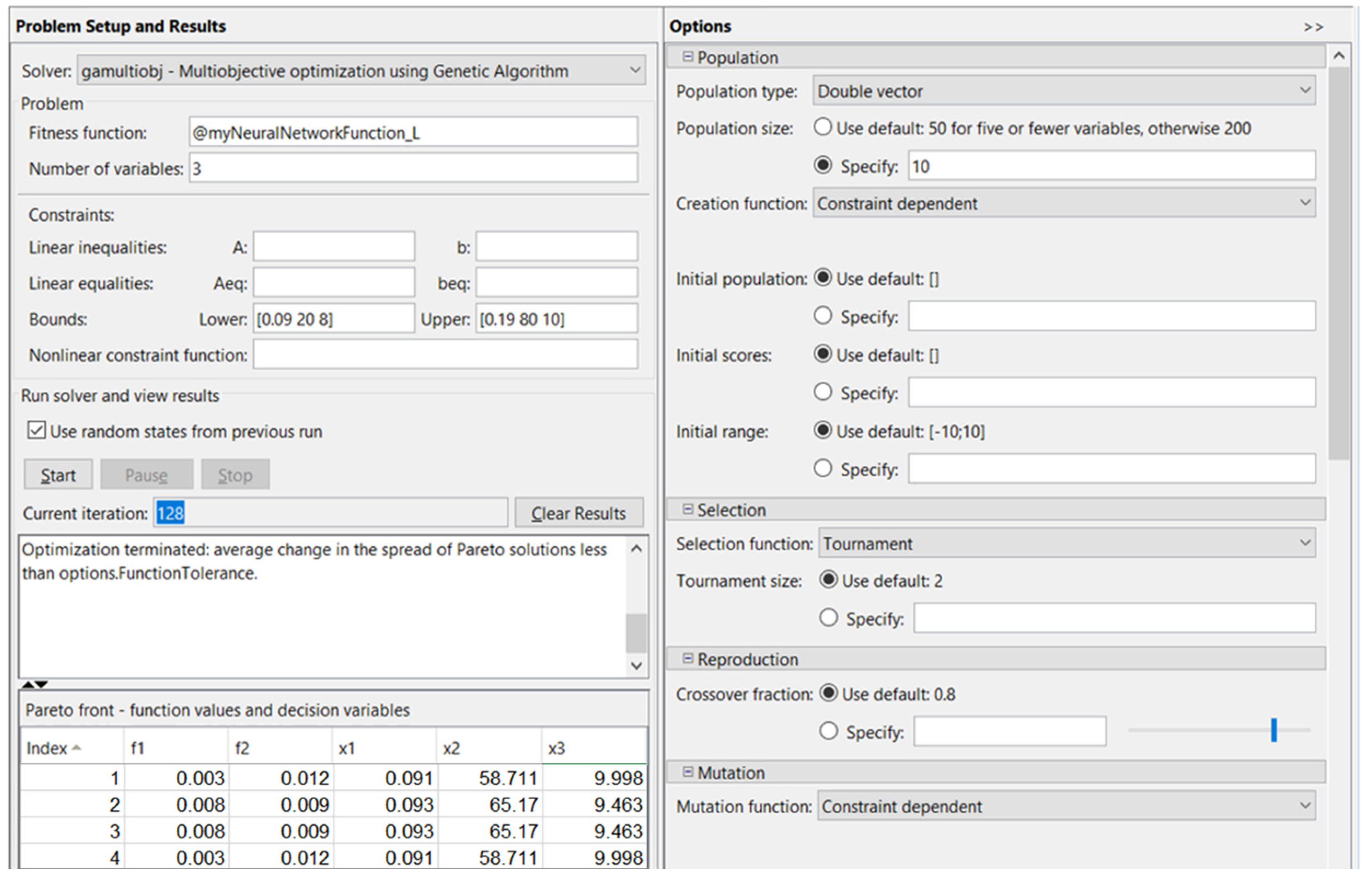
By optimization using the genetic algorithm, after 128 iterations, in the case corresponding to diameter l, L, the optimized conditions were obtained, as shown in Figure 8.
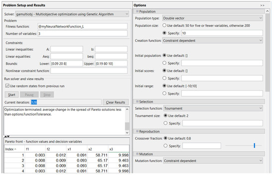
Figure 8.
Optimization using the genetic algorithm for l, L.
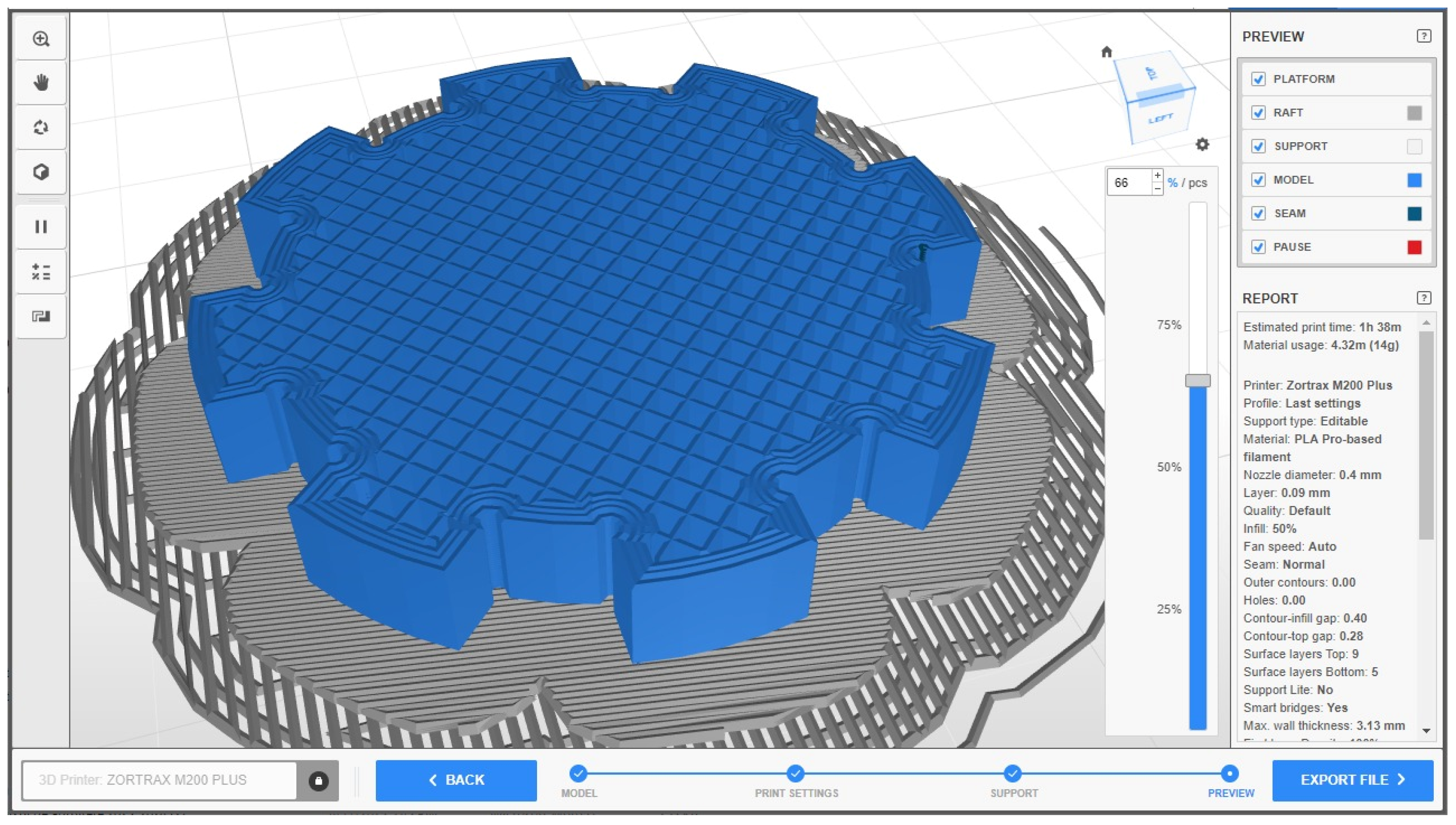
In order to verify and validate the results obtained by multi-objective optimization using the genetic algorithm, a new sample was realized with the following parameters (which can be chosen on the 3D printer, with values close to the optimal ones): 0.09 for the layer thickness, 50 for the infill density, 50 for the Ød1 nominal diameter, 42 for the Ød2 nominal diameter, and 10 for l (Figure 9). For the hub, the printing values were the same.

Figure 9.
Printing process simulated with Z-Suite software for the new sample.
The predicted values using the three neural networks for absolute relative deviations are presented in Table 9.
Table 9.
The predicted values for absolute relative deviations.
In this situation, the measured value for the samples and the values for absolute relative deviations are presented in Table 10.
Table 10.
The measured value for the samples and the values for absolute relative deviations.
Thus, the research presented in this article has been experimentally validated, demonstrating the effectiveness of the proposed optimization approach and the accuracy of the predictive models.
4.4. Identified Patterns and Trends in Dimensional Deviations
The artificial neural network (ANN) analysis revealed key patterns and trends regarding the influence of layer thickness, infill density, and nominal diameter on dimensional deviations in FDM-printed spline shafts and hubs. The genetic algorithm further optimized these parameters to minimize deviations.
Layer thickness: The ANN identified that smaller layer thickness values generally lead to lower dimensional deviations due to improved print resolution. However, excessively small layer thicknesses increase the printing time and may lead to material inconsistencies. The genetic algorithm optimized this trade-off, identifying an optimal range where accuracy is maximized without significantly increasing production time.
Infill density: The results indicated that higher infill densities contribute to better structural integrity, reducing shrinkage-related deviations. However, after a certain threshold, increasing infill density had a diminishing effect on accuracy improvements while increasing material consumption. The genetic algorithm determined an optimal infill percentage that balances accuracy and material efficiency.
Nominal diameter: The ANN detected those deviations varied across different spline nominal diameters. Larger nominal diameters tended to exhibit lower percentage deviations due to improved stability during printing. However, deviations were more unpredictable for smaller nominal diameters, requiring tighter process control. The optimization algorithm provided recommendations for suitable diameter ranges that minimize errors.
5. Conclusions
This study presents a comprehensive analysis of dimensional deviations in FDM-printed splined shafts and hubs, highlighting the key parameters influencing accuracy. The main conclusions drawn from the research are as follows:
Printing parameters significantly affect dimensional accuracy—layer thickness, infill density, and nominal diameter contribute to deviations, with lower layer thickness generally improving precision.
Artificial neural networks (ANNs) provide reliable predictions—the ANN models trained in this study achieved high accuracy, with correlation coefficients above 0.91, proving their effectiveness in predicting dimensional deviations.
Genetic algorithm (GA) optimization enhances accuracy—multi-objective optimization allowed for the identification of the best printing conditions, reducing deviations and improving manufacturing consistency.
Measurement and validation confirm model reliability—CMM-based dimensional measurements and statistical validation confirmed that optimized printing conditions yield improved precision.
Future work should focus on extending the methodology to other materials and exploring additional post-processing techniques to further reduce dimensional variations.
This study demonstrates that combining experimental analysis with ANN and GA optimization provides a powerful approach for improving the dimensional accuracy of FDM-printed mechanical components, ensuring better performance in real-world applications.
We acknowledge that the optimized spline configuration obtained through our study deviates from the standardized combinations defined in ISO 14. This deviation arises as a result of the optimization process, which aims to minimize dimensional deviations in FDM-printed spline shafts and hubs rather than adhere strictly to existing standards.
It is important to emphasize that our research does not seek to propose an alternative to ISO 14 but rather to demonstrate how process optimization in additive manufacturing can impact dimensional accuracy. The methodology presented may be particularly useful in non-standard applications where flexibility in spline design is acceptable, such as prototyping, lightweight structures, or cases where conventional manufacturing constraints do not apply.
Author Contributions
A.-D.R. and D.-C.A., conceptualization; A.-D.R., D.-C.A. and C.-F.B., methodology; D.-C.A. and T.G., software and 3D models; A.-D.R., D.-C.A., A.S. and C.-F.B., data analysis and writing the paper; D.-C.A., review and editing. All authors have read and agreed to the published version of the manuscript.
Funding
This research received no external funding.
Institutional Review Board Statement
Not applicable.
Informed Consent Statement
Not applicable.
Data Availability Statement
The data presented in this study are available within the article.
Conflicts of Interest
The authors declare no conflicts of interest.
References
- Gibson, I.; Rosen, D.W.; Stucker, B. Additive Manufacturing Technologies. In 3D Printing, Rapid Prototyping, and Direct Digital Manufacturing, 2nd ed.; Springer: Berlin/Heidelberg, Germany, 2015. [Google Scholar]
- Stojković, J.R.; Turudija, R.; Vitković, N.; Górski, F.; Păcurar, A.; Pleşa, A.; Ianoşi-Andreeva-Dimitrova, A.; Păcurar, R. An Experimental Study on the Impact of Layer Height and Annealing Parameters on the Tensile Strength and Dimensional Accuracy of FDM 3D Printed Parts. Materials 2023, 16, 4574. [Google Scholar] [CrossRef] [PubMed]
- Mohamed, O.A.; Masood, S.H.; Bhowmik, J.L. Modeling, analysis, and optimization of dimensional accuracy of FDM-fabricated parts using definitive screening design and deep learning feedforward artificial neural network. Adv. Manuf. 2021, 9, 115–129. [Google Scholar] [CrossRef]
- Karad, A.S.; Sonawwanay, P.D.; Naik, M.; Thakur, D.G. Experimental study of effect of infill density on tensile and flexural strength of 3D printed parts. J. Eng. Appl. Sci. 2023, 70, 104. [Google Scholar]
- Vora, H.D.; Sanyal, S. A comprehensive review: Metrology in additive manufacturing and 3D printing technology. Prog. Addit. Manuf. 2020, 5, 319–353. [Google Scholar] [CrossRef]
- Boschetto, A.; Bottini, L. Accuracy prediction in fused deposition modeling. Int. J. Adv. Manuf. Technol. 2014, 73, 913–928. [Google Scholar] [CrossRef]
- Mohamed, O.A.; Masood, S.H.; Bhowmik, J.L. Mathematical modeling and FDM process parameters optimization using response surface methodology based on Q-optimal design. Appl. Math. Model. 2016, 40, 10052–10073. [Google Scholar]
- Eryıldız, M. Effect of build orientation on mechanical behaviour and build time of FDM 3D-printed PLA parts: An experimental investigation. Eur. Mech. Sci. 2021, 5, 116–120. [Google Scholar]
- Pant, M.; Singari, R.M.; Arora, P.K.; Moona, G.; Kumar, H. Wear assessment of 3–D printed parts of PLA (polylactic acid) using Taguchi design and Artificial Neural Network (ANN) technique. Mater. Res. Express 2020, 7, 115307. [Google Scholar] [CrossRef]
- Darbar, R.; Patel, P.M. Optimization of fused deposition modeling process parameter for better mechanical strength and surface roughness. Int. J. Mech. Eng. 2017, 6, 7–18. [Google Scholar]
- Camposeco-Negrete, C. Optimization of FDM parameters for improving part quality, productivity and sustainability of the process using Taguchi methodology and desirability approach. Prog. Addit. Manuf. 2020, 5, 59–65. [Google Scholar] [CrossRef]
- Anghel, D.C.; Iordache, D.M.; Rizea, A.D.; Stanescu, N.D. A New Approach to Optimize the Relative Clearance for Cylindrical Joints Manufactured by FDM 3D Printing Using a Hybrid Genetic Algorithm Artificial Neural Network and Rational Function. Processes 2021, 9, 925. [Google Scholar] [CrossRef]
- Sood, A.K.; Ohdar, R.K.; Mahapatra, S.S. Parametric appraisal of fused deposition modelling process using the grey Taguchi method. Proc. Inst. Mech. Eng. Part B J. Eng. Manuf. 2010, 224, 135–145. [Google Scholar] [CrossRef]
- Sood, A.K.; Ohdar, R.K.; Mahapatra, S.S. Parametric appraisal of mechanical property of fused deposition modelling processed parts. Mater. Des. 2010, 31, 287–295. [Google Scholar] [CrossRef]
- Sood, A.K.; Chaturvedi, V.; Datta, S.; Mahapatra, S.S. Optimization of process parameters in fused deposition modeling using weighted principal component analysis. J. Adv. Manuf. Syst. 2011, 10, 241–259. [Google Scholar] [CrossRef]
- Sood, A.K.; Ohdar, R.K.; Mahapatra, S.S. Experimental investigation and empirical modelling of FDM process for compressive strength improvement. J. Adv. Res. 2012, 3, 81–90. [Google Scholar] [CrossRef]
- Sood, A.K.; Equbal, A.; Toppo, V.; Ohdar, R.K.; Mahapatra, S.S. An investigation on sliding wear of FDM built parts. CIRP J. Manuf. Sci. Technol. 2012, 5, 48–54. [Google Scholar] [CrossRef]
- Equbal, A.; Sood, A.K.; Toppo, V.; Ohdar, R.K.; Mahapatra, S.S. Prediction and analysis of sliding wear performance of fused deposition modelling-processed ABS plastic parts. Proc. Inst. Mech. Eng. Part J J. Eng. Tribol. 2010, 224, 1261–1271. [Google Scholar] [CrossRef]
- Sahu, R.K.; Mahapatra, S.S.; Sood, A.K. A study on dimensional accuracy of fused deposition modeling (FDM) processed parts using fuzzy logic. J. Manuf. Sci. Prod. 2013, 13, 183–197. [Google Scholar] [CrossRef]
- Padhi, S.K.; Sahu, R.K.; Mahapatra, S.S.; Das, H.C.; Sood, A.K.; Patro, B.; Mondal, A.K. Optimization of fused deposition modeling process parameters using a fuzzy inference system coupled with Taguchi philosophy. Adv. Manuf. 2017, 5, 231–242. [Google Scholar] [CrossRef]
- Mohanty, A.; Nag, K.S.; Bagal, D.K.; Barua, A.; Jeet, S.; Mahapatra, S.S.; Cherkia, H. Parametric optimization of parameters affecting dimension precision of FDM printed part using hybrid Taguchi-MARCOS-nature inspired heuristic optimization technique. Mater. Proc. 2022, 50, 893–903. [Google Scholar] [CrossRef]
- Haghighi, A.; Li, L. Study of the relationship between dimensional performance and manufacturing cost in fused deposition modeling. Rapid Prototyp. J. 2018, 24, 395–408. [Google Scholar] [CrossRef]
- Dey, A.; Yodo, N. A Systematic Survey of FDM Process Parameter Optimization and Their Influence on Part Characteristics. J. Manuf. Mater. Process. 2019, 3, 64. [Google Scholar] [CrossRef]
- Asadollahi-Yazdi, E.; Gardan, J.; Lafon, P. Toward integrated design of additive manufacturing through a process development model and multi-objective optimization. Int. J. Adv. Manuf. Technol. 2018, 96, 4145–4164. [Google Scholar] [CrossRef]
- Mahmood, S.; Qureshi, A.; Talamona, D. Taguchi based process optimization for dimension and tolerance control for fused deposition modelling. Addit. Manuf. 2018, 21, 183–190. [Google Scholar] [CrossRef]
- Wang, Y.; Jun-Tong, X.; Jin, Y. A model research for prototype warp deformation in the FDM process. Int. J. Adv. Manuf. Technol. 2007, 33, 1087–1096. [Google Scholar] [CrossRef]
- Bahnini, I.; Anghel, D.C.; Rizea, A.D.; Zaman, U.K.; Siadat, A. Accuracy Investigation of Fused Deposition Modelling (FDM) Processed ABS and ULTRAT Parts. Int. J. Manuf. Mater. Mech. Eng. 2022, 12, 1–19. [Google Scholar] [CrossRef]
- Petruse, R.E.; Simion, C.; Bondrea, I. Geometrical and Dimensional Deviations of Fused Deposition Modelling (FDM) Additive-Manufactured Parts. Metrology 2024, 4, 411–429. [Google Scholar] [CrossRef]
- Sawant, D.A.; Shinde, B.M.; Raykar, S.J. Post processing techniques used to improve the quality of 3D printed parts using FDM: State of art review and experimental work. Mater. Today Proc. 2023, in press. [CrossRef]
- Gradinaru, S.; Tabaras, D.; Gheorghe, D.; Gheorghita, D.; Zamfir, R.; Vasilescu, M.; Dobrescu, M.; Grigorescu, G.; Cristescu, I. Analysis of the anisotropy for 3D printed pla parts usable in medicine. Univ. Politech. Buchar. Sci. Bull. Ser. B Chem. Mater. Sci. 2019, 81, 313–324. [Google Scholar]
- Simion, I.; Arion, A.F. Dimensioning rules for 3D printed parts using additive technologies (FDM). Univ. Politech. Buchar. Sci. Bull. Ser. D 2016, 78, 79–92. [Google Scholar]
- Maurya, A.K.; Kumar, A. Study the microhardness and surface roughness of as-built and heat-treated additive manufactured IN718 alloy. Univ. Politech. Buchar. Sci. Bull. Ser. D 2022, 84, 211–224. [Google Scholar]

Disclaimer/Publisher’s Note: The statements, opinions and data contained in all publications are solely those of the individual author(s) and contributor(s) and not of MDPI and/or the editor(s). MDPI and/or the editor(s) disclaim responsibility for any injury to people or property resulting from any ideas, methods, instructions or products referred to in the content. |
© 2025 by the authors. Licensee MDPI, Basel, Switzerland. This article is an open access article distributed under the terms and conditions of the Creative Commons Attribution (CC BY) license (https://creativecommons.org/licenses/by/4.0/).