Abstract
Using COMSOL finite element software, a three-dimensional numerical transient model of an underground tunnel collapse vertical freezing repair project was established. The model was altered to change the head difference, allowing for analysis of the development of the permafrost curtain, the time of intersection circles, and the freezing temperature field cloud diagram. The results indicated that, without seepage, development of the upstream and downstream permafrost curtains was stable and uniform. However, under seepage conditions, development of the upstream and downstream permafrost curtains became increasingly uneven with increasing seepage velocity. The downstream side of the soil body began freezing earlier than the upstream side, and the final temperature was lower. The intersection time of the freezing wall was an important indicator of development of the permafrost curtain, and the freezing time of the freezing wall was the most critical indicator. A hydraulic head difference of 1 m was found to significantly impact the development of the freezing wall, with less influence from seepage velocity on the overall permafrost curtain intersection time. However, the intersection time of the isotherm increased significantly with increasing seepage flow rate. The findings from this project provide a theoretical reference for future restoration design.
1. Introduction
Since the 20th century, the rapid economic development of cities, coupled with the gradual expansion of urbanization and the resulting population pressure and insufficient space above ground, has led to the full development and utilization of underground space as a preferred method to address these issues in many countries. Underground tunnels, which are engineering structures widely used in the ground, represent an efficient use of underground space. However, when constructing urban tunnels through saturated, water-rich, soft ground, the density of urban buildings necessitates the prevention of groundwater seepage during tunnel construction without affecting surrounding buildings, as well as the prevention of collapse accidents during the excavation of underground tunnels. Thus, meeting the high requirements of urban tunnel construction presents a challenging problem that needs to be solved [1,2,3,4]. Artificial ground freezing (AGF) technology is a method that uses freezing pipes to lower the temperature of the soil around the area to be excavated, gradually reducing the natural soil temperature to become permafrost, forming a permafrost body with a certain strength [5,6,7,8,9]. This technology, after a certain period of active freezing, can form a stable and solid frozen soil curtain, which can prevent the flow of groundwater. Under its support, the construction of underground projects can be completed safely and efficiently. Therefore, the artificial ground freezing method (AGF) has become one of the important engineering techniques for underground engineering research, and its reinforcement of the soil to be excavated and excellent water sealing properties have important engineering value [10,11,12,13,14,15,16]. In recent years, scholars at home and abroad have reported relevant achievements in the study of artificial ground freezing in underground restoration projects. Liu et al. [17], in conjunction with the repair project of Shanghai Metro Line 4, used the horizontal freezing method to repair collapsed tunnels and analyzed the impact of each construction process on the temperature of the permafrost wall. Through on-site measurement and analysis, the results showed that temperature is an important index to judge the characteristics of the permafrost wall. By reasonably arranging temperature monitoring points and adopting informationized temperature monitoring, the development of the freezing wall can be grasped, ensuring the safety of freezing method–based construction. Hu et al. [18], in the context of submarine fault shield repair construction, considered the adverse effect of the salt content of seawater on freezing, such as reducing the thickness of the permafrost curtain and decreasing its strength. The freezing program was specifically designed with measurement of the freezing and construction process in mind. Through calculation and analysis of permafrost temperature monitoring data, it was shown that the hood-shaped permafrost curtain achieved good results in submarine shield repair, verifying the feasibility of this freezing scheme in submarine shield tunnel repair. Hao and Shi [19], for shield tunnel construction under the river, after the occurrence of sudden water and sand accidents, used the filling and freezing method to form a temporary freezing blocking wall and then discharged the water inside the tunnel to construct a permanent blocking wall for the next step of the tunnel project, providing a guarantee for the safety of the construction of the tunnel project and the smooth progress of the project. Practice shows that use of the filling and freezing method for the construction of temporary blocking walls in complex geological conditions can effectively prevent the occurrence of sudden water and sand accidents, meaning personnel do not need to enter the water tunnel under construction, which results in high controllability and safety, as we; as the popularity and widespread application of this approach. Xiao et al. [20] introduced the use of horizontal freezing technology to repair tunnels, using vertical sealing water retaining soil and horizontal freezing of the concealed excavation in a project involving destruction of a tunnel and construction of an intact tunnel connection section, with the repair project being successful. Chu et al. [21], in conjunction with the Sichuan gas east pipeline project Wuhan Yangtze River shield crossing project, tracked and monitored aspects such as freezing brine temperature, permafrost temperature, and groundwater level at Wenkong. Through analyzing and researching the monitoring results, they obtained dynamic data regarding frozen brine temperature, frozen soil temperature, and hydrological borehole water level, and put forward a proposal for tunnel repair and freezing construction on this basis. Xiao et al. [22] detailed the use of a four-row pipe local freezing method to repair subway tunnels, and monitored and analyzed the site freezing temperature, freezing force, and so on. The analyzed results showed that the quality of the freezing method is affected by temperature. By reasonably arranging temperature monitoring points, adopting informationized construction, and mastering changes in temperature, the safety of freezing construction as a part of complex projects can be ensured.
Upon reviewing the relevant literature, it is evident that the artificial ground freezing method has been widely applied in tunnel rehabilitation projects. Experts and scholars have delved into the mechanism of reinforcement through numerical simulations and on-site measurements, examining the temperature field, freezing expansion, and thawing sinking rules, thereby establishing a comprehensive freezing theory. However, there is a dearth of research on the vertical freezing method. Consequently, it is imperative to investigate the temperature and freezing degree fields of the vertical freezing method in tunnel rehabilitation projects. This study aimed to explore the development and change laws of the temperature field of the vertical freezing method, offering a foundation for future tunnel repair projects. Utilizing an underground collapsed tunnel freezing reinforcement repair project as a case study, in this study we constructed a three-dimensional water-heat coupling model to examine the frozen permafrost curtain and temperature field development and distribution under different seepage conditions. Through dynamic simulations of the evolution of the permafrost curtain, the findings from this project can serve as a theoretical basis for the design of similar projects in the future.
2. Vertical Freezing Program Design
2.1. Project Overview
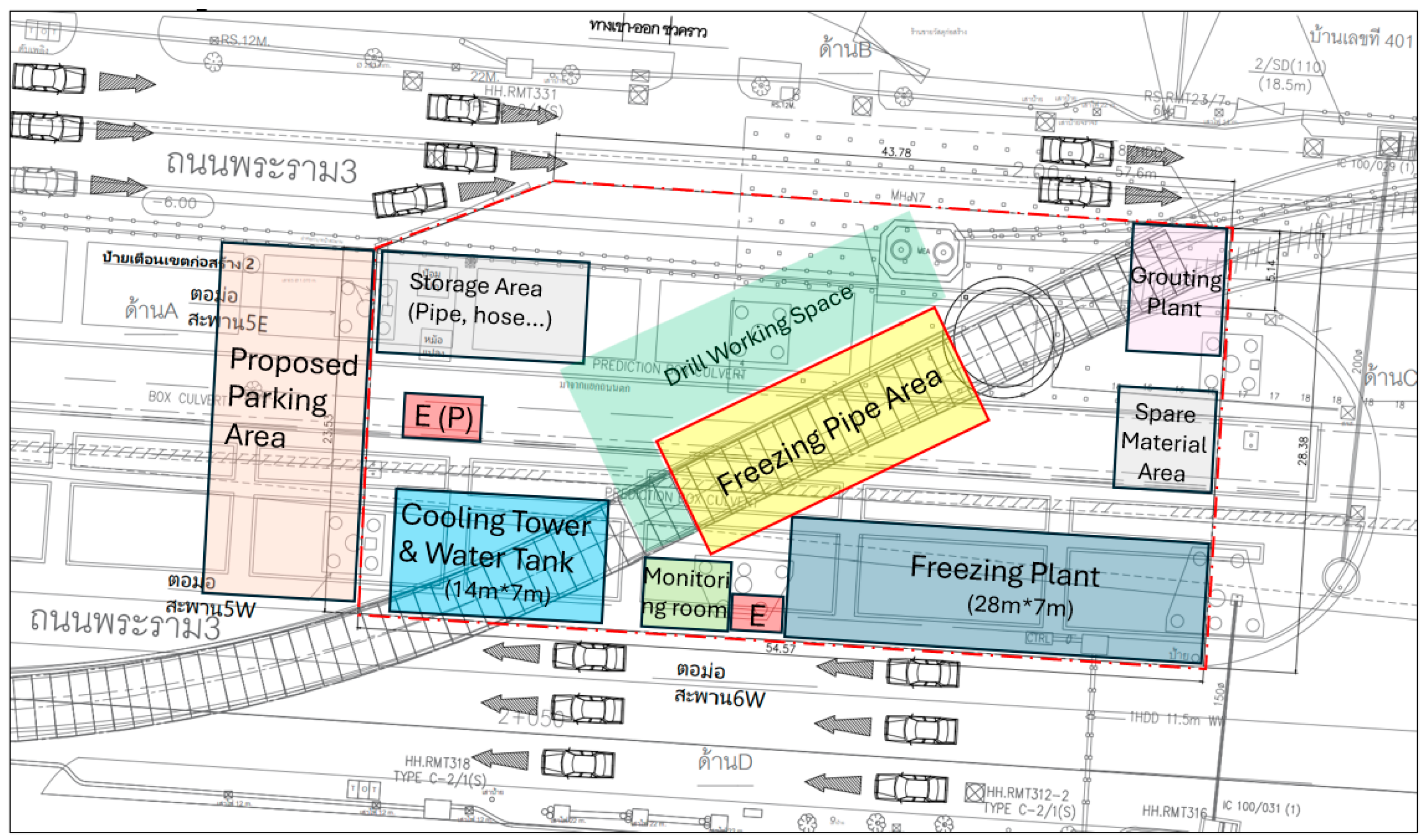
This study focused on a tunnel collapse repair project connecting two shafts, where the length of the collapsed section reached 16.9 m, with the centerline of the tunnel situated at a ground level of −26.55 m. Given that the tunnel collapse was situated near elevated piers, the surrounding environment was sensitive, and the unique geographical context did not favor an open-cut repair method. Therefore, the preferred approach was to reinforce the soil at the collapse site through vertical freezing, followed by concealed excavation repair. The freezing repair method addresses the problematic layers of powdery clay, fine sand with strong permeability, and other unfavorable soils. Consequently, it is crucial to manage groundwater flow during the freezing repair process. Figure 1 illustrates the surrounding environment of the freezing area.
Figure 1.
Overview of the project.
2.2. Arrangement of Freezing Pipes
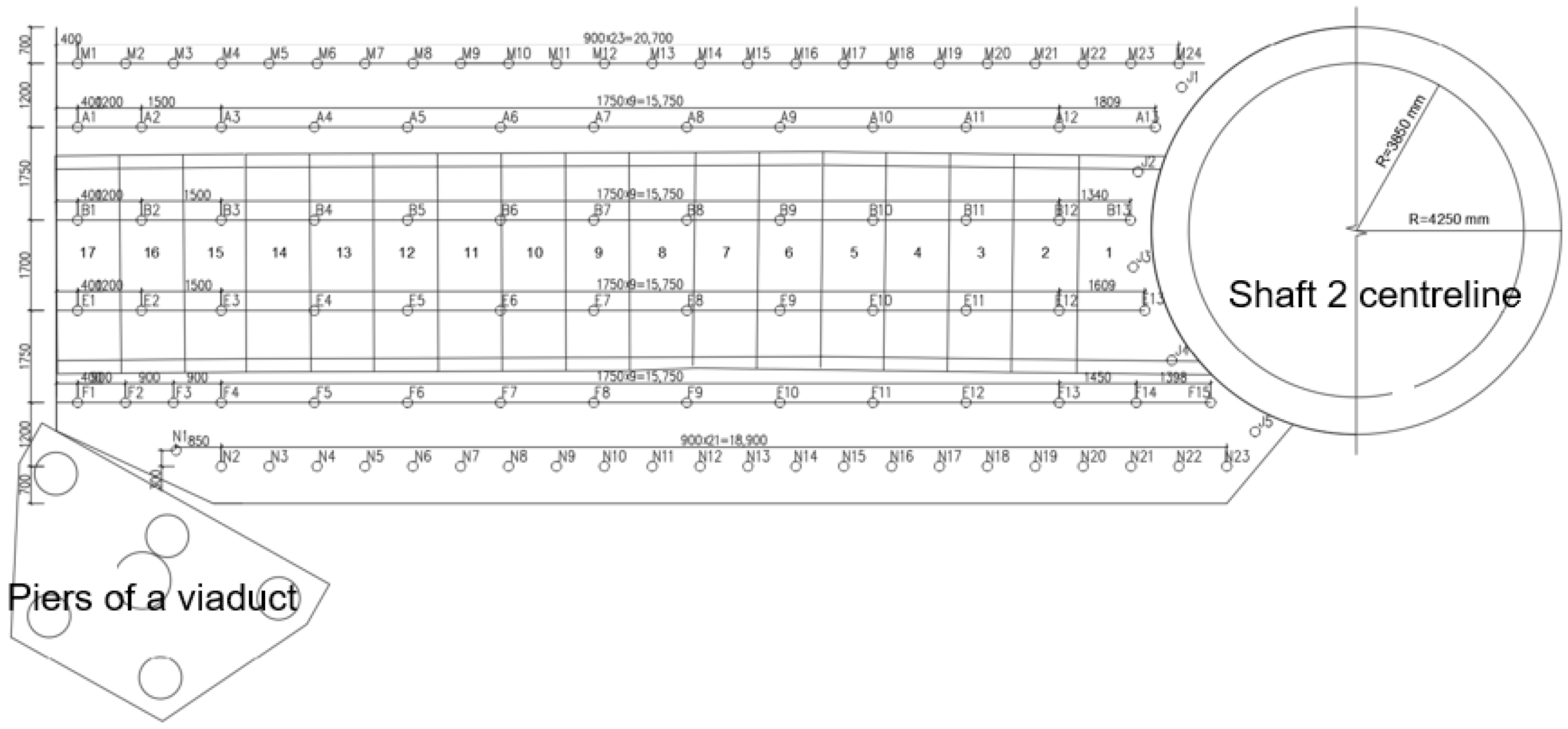
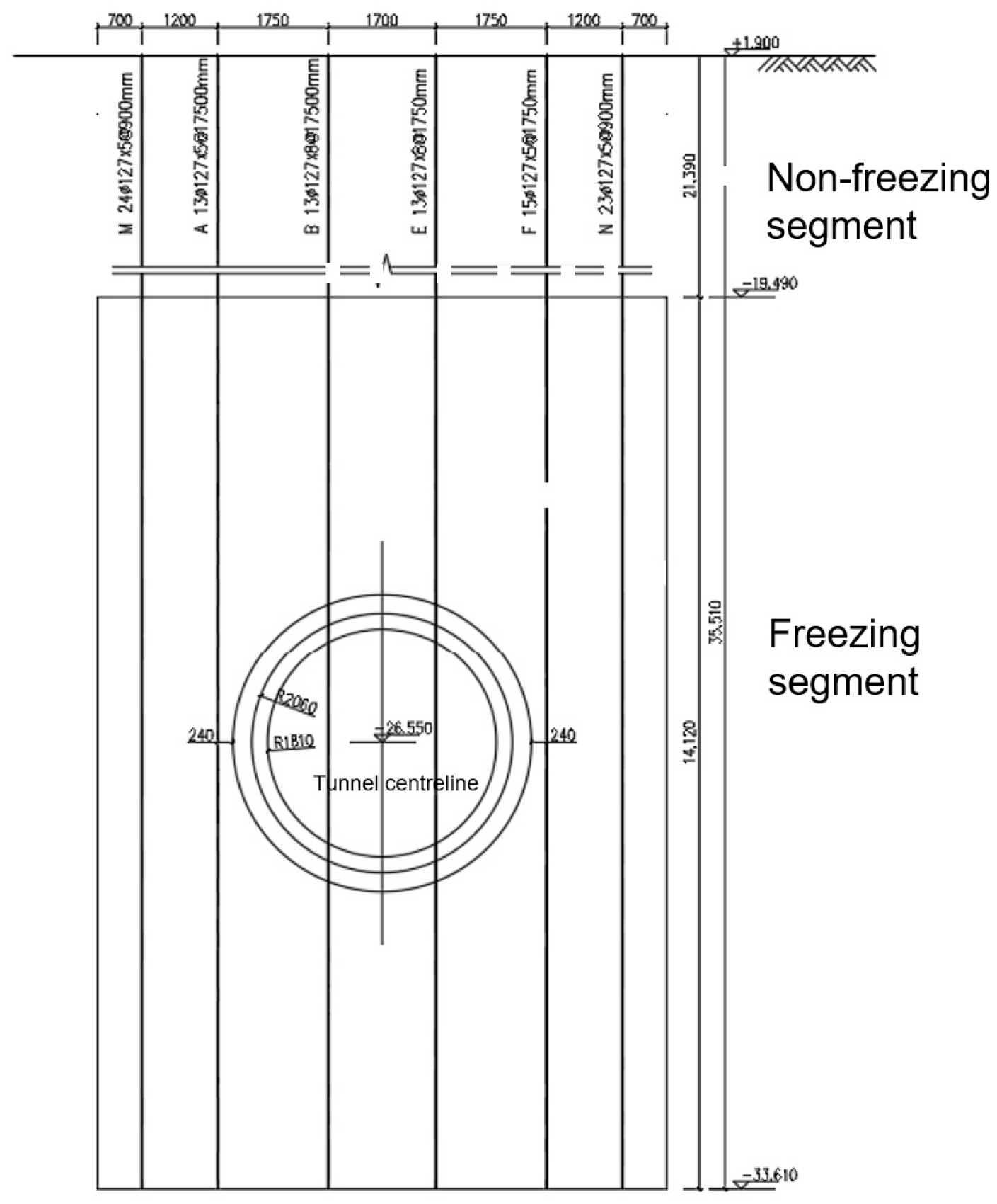
To enhance the impact of freezing pipes on the surrounding soil, given that the collapsed tunnel was situated near the viaduct pier, the vertical freezing method was selected for soil reinforcement. The freezing pipes, with a total length of 35.51 m, were vertically inserted from the ground to the collapsed tunnel. These pipes were divided into local freezing and non-freezing sections, with the former measuring 14.12 m and the latter 21.39 m. The diameter of all freezing pipes was 127 mm, and a total of 106 pipes were laid out. The inner diameter of the shafts was 3.85 m, and the outer diameter was 4.25 m. The freezing pipes, each with a diameter of 127 mm, were inserted from elevation +1.9 m to elevation −33.61 m. The pipes in the partial freezing section traversed the entire collapsed area of the tunnel. Figure 2 illustrates the plan layout of the freezing pipes, while Figure 3 presents a cross-section of the freezing pipes.
Figure 2.
Plan layout of the freezing pipes.

Figure 3.
Cross-section of freezing pipe arrangement.
3. Establishment of Finite Element Numerical Simulations
3.1. Fundamental Assumption
The numerical model represents a hydrothermal coupling mechanism, accounting for the intricate action mechanism of porous media under conditions of seepage and freezing. Building upon relevant foundational principles, the model was established under the following basic assumptions [23,24]:
- 1.
- The analysis herein neglects the influence of stress and displacement fields on the temperature field, focusing solely on the hydrothermal interaction between seepage and temperature fields.
- 2.
- It is assumed that the soil constitutes a saturated, homogeneous, isotropic porous medium with a constant total porosity.
- 3.
- Thermal-physical properties within the soil layers are considered constant across layers.
- 4.
- The impact of solute concentration on the freezing point is negligible, and ice is assumed to be stationary, without deformation.
- 5.
- It is assumed that the initial temperature of the stratum is 18 °C, the soil is a porous saturated medium, and the soil is homogeneously distributed and homogeneous.
3.2. Model Calculation Theory
3.2.1. Temperature Field Theory
According to the basic theory of heat transfer, in the freezing process, the soil and low-temperature refrigerant exchange heat form permafrost. Seepage within the soil is frozen into ice, which is a heat transfer problem with a phase change. The heat transfer of the porous medium is related to conduction, convection, and other factors, and the seepage conditions of the transient temperature field heat conduction can be calculated using the following equation:
where subscripts S and f are solid and fluid, respectively; ∇ is the Hamiltonian operator; T is the temperature; C is the specific heat capacity; is the density in kg/m−3; is the convective velocity; keff is the thermal conductivity; is the solid volume fraction; and Q is the other heat source sink term.
3.2.2. Percolation Field Theory
When determining seepage field flow direction, flow rate is determined by the boundary head difference. Because the soil body is a porous medium, its geometry is complex, and seepage through the pore channel is discontinuous and exhibits a slow flow rate. Therefore, seepage flow in the porous medium usually consists of laminar flow or nearly laminar flow, which is subject to Darcy’s law. The formula is:
where the subscript t denotes time; ∇ is the Hamiltonian operator; ∇P is the pressure gradient; Qm is the water source term; K is the infiltration rate of soil; is the water viscosity; is the water density; and is the Darcy seepage rate.
3.2.3. Theory of Coupled Temperature and Seepage Fields
In the model boundary, the head difference is set to produce unidirectional seepage. When the seepage flows through the porous media, this produces heat exchange, in which heat will be diffused with the seepage flow, resulting in uneven distribution of the temperature field. When the temperature field changes, due to the permeability coefficient of the porous media other physical parameters will change. Temperature induces a functional relationship, so that the inverse effect of the temperature field on the seepage field achieves bi-directional coupling, and the temperature field is coupled with the seepage field. The coupling of temperature field to seepage field involves dynamic adjustment of heat and fluid in porous media. In this study, the Heaviside function was used to describe the coupling relationship between the permeability coefficient and the temperature in the process of the ice–water phase transition, and the unit leap order function is established as:
where subscripts u and f are unfrozen and frozen soil, respectively; K is the permeability coefficient; T is the soil temperature, Td is the critical temperature of ice-water phase transition; and dT is the ice-water phase transition gap.
3.3. Geometric Modeling and Parameter Selection
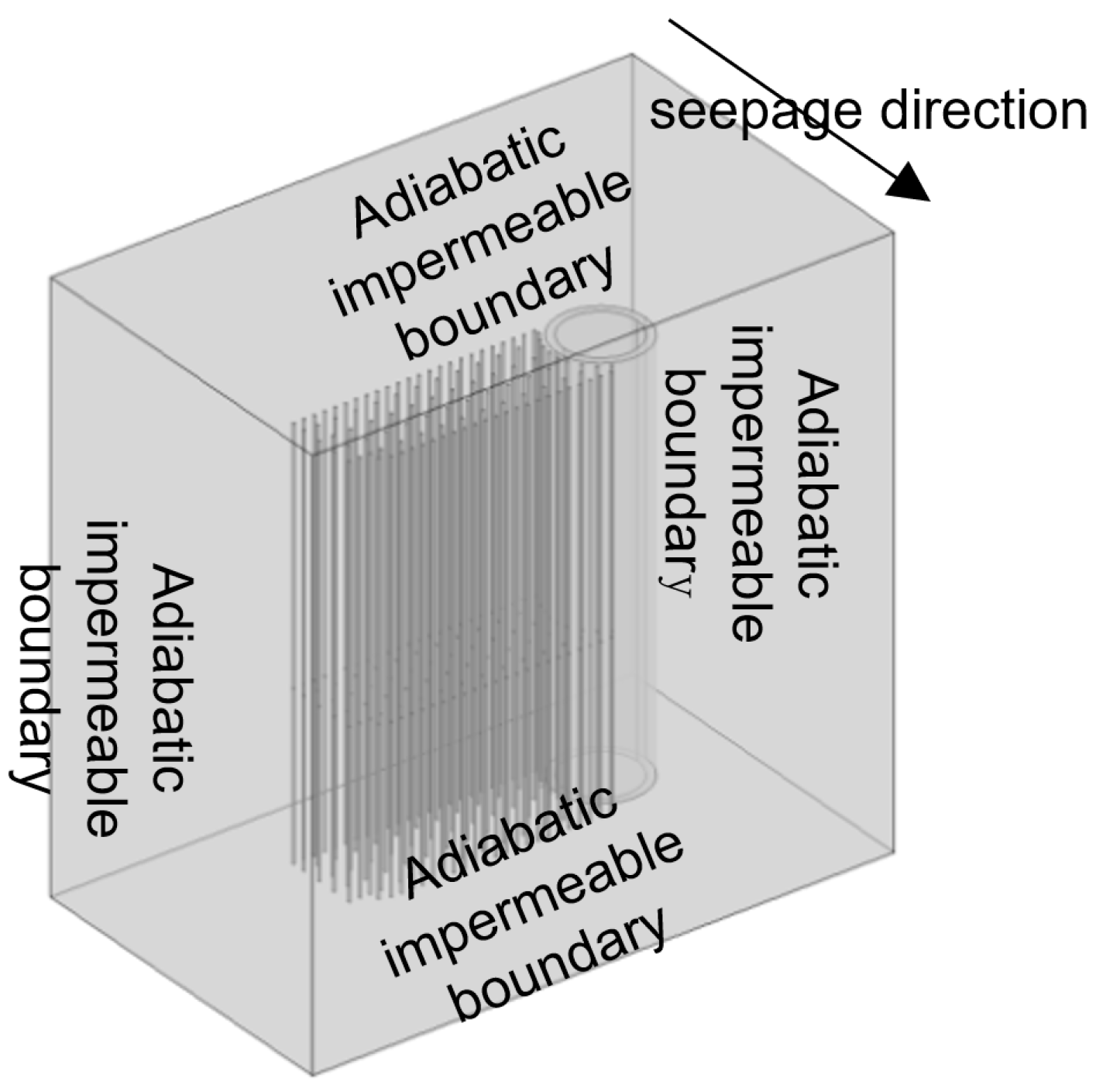
(1) A three-dimensional transient model was established using COMSOL finite element software, with the geometric model’s dimensions determined by the freezing range and the impact of groundwater flow on the permafrost curtain. The model, with dimensions of L(X) × W(Y) × H(Z) = 50 m × 30 m × 50 m, was meshed using a physical field control model to ensure accurate representation of the temperature field and minimize boundary error. The model was surrounded by an adiabatic boundary, initially set at 18 °C, with impermeable boundaries on the top, bottom, left, and right sides, and permeable boundaries on the front and back. The meshing and boundary conditions are illustrated in Figure 4 and Figure 5, respectively.
Figure 4.
Grid division diagram.

Figure 5.
Boundary condition diagram.
(2) In this study, the soil parameters chosen were derived from the least favorable soil layer of the project, drawing upon relevant permafrost experimental research [25,26] to ascertain the thermal conductivity, the permeability coefficient of the soil, and other pertinent properties. The values of the selected parameters for the physical model are presented in Table 1.

Table 1.
Relevant parameter values.
(3) During the freezing period, the soil undergoes a phase change into frozen soil due to the influence of low temperatures. The thermal conductivity, permeability coefficient, specific heat, and density of the soil are temperature-dependent, with the unfrozen temperature range extending from 0 °C to 30 °C and the frozen temperature range from −30 °C to 0 °C. The design specifications dictate that the brine temperature serves as the temperature load. The model employs transient analysis, with the wall of the frozen pipe serving as the thermal load boundary condition, and the surrounding environment set to an adiabatic boundary. The freezing process was discretized into 60 day-long time steps, each of 24 h. The brine cooling schedule was achieved through interpolation of a function. Specifically, within the first 5 days of freezing, the refrigerant temperature was reduced to −15 °C, and between days 10 and 60, the refrigerant temperature dropped to −28 °C. The temperature reduction schedule during freezing is detailed in Table 2.
Table 2.
Salt water cooling program.
4. Analysis of Numerical Simulation Results
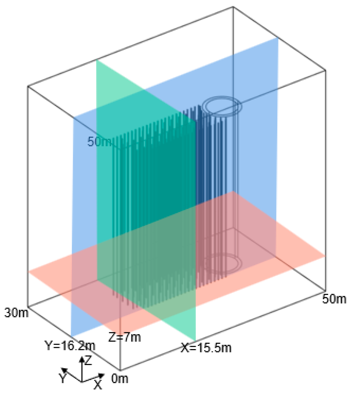
To enhance understanding of the impact of varying seepage velocities on the three-dimensional temperature field of the freezing method, three sections—X, Y, and Z—were chosen for analysis of temperature field cloud isothermograms. Given the significance of the Z section in the study, a more detailed analysis of its numerical simulation results was performed. The precise locations of these sections in the three directions are illustrated in Figure 6.
Figure 6.
Schematic representation of the location of the profiles in different directions.
4.1. Freezing Temperature Field and Permafrost Curtain Development Pattern in the Z-Section
4.1.1. Z-Section Without Considering the Seepage Flow Scenario
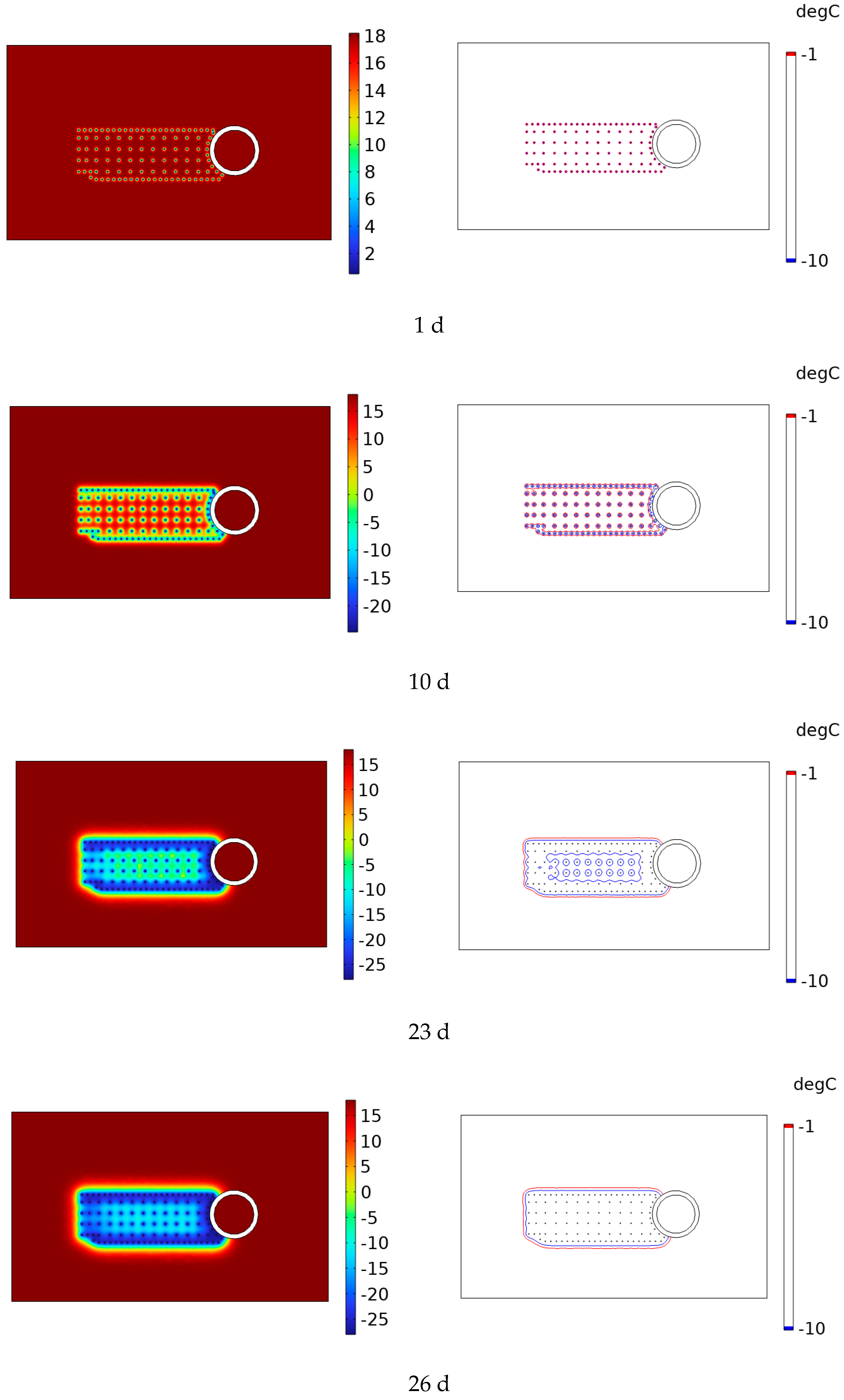
When determining a scenario without seepage in the soil body, the head difference between the upstream and downstream boundaries of the model was set to 0 m, focusing solely on the heat transfer process within the porous medium. The temperature field and isotherm maps at −1 °C and −10 °C from the numerical simulation results without seepage are depicted in Figure 7. As illustrated in Figure 7, at the onset of the freezing period (1 d), the minimal cold generated by the freezing pipe was not propagated to distant areas. The isotherm map indicates that the permafrost curtain was not yet formed in the immediate vicinity of the freezing pipe. By the 10th day of freezing, the cold produced by the freezing pipe, which had been accumulating over time, began to transfer to warmer areas. At this stage, the frozen area adjacent to the shaft side and parts of the upper side of the −1 °C isotherm exhibited partial intersection with the circle, gradually defining the outline of the frozen soil curtain. By the 23rd day of freezing, it was evident that the majority of the frozen area had reached the freezing temperature. At this point, the −1 °C isotherm of the entire frozen area had completed its circular intersection, with the frozen curtain nearly fully formed. The outer side of the −10 °C isotherm had completed the circular intersection, while the inner side showed incomplete circles, likely due to the less densely packed freezing pipes on the inner side. After 26 days of active freezing, all −10 °C isotherms had completed their circular intersections, and the overall permafrost curtain had been fully closed. As the freezing period continued to lengthen, the permafrost curtain entered a stable development phase, expanding uniformly in all directions.

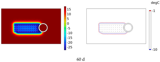
Figure 7.
Temperature field cloud and isotherm maps at different times.
4.1.2. Z-Section Considering Seepage Flow
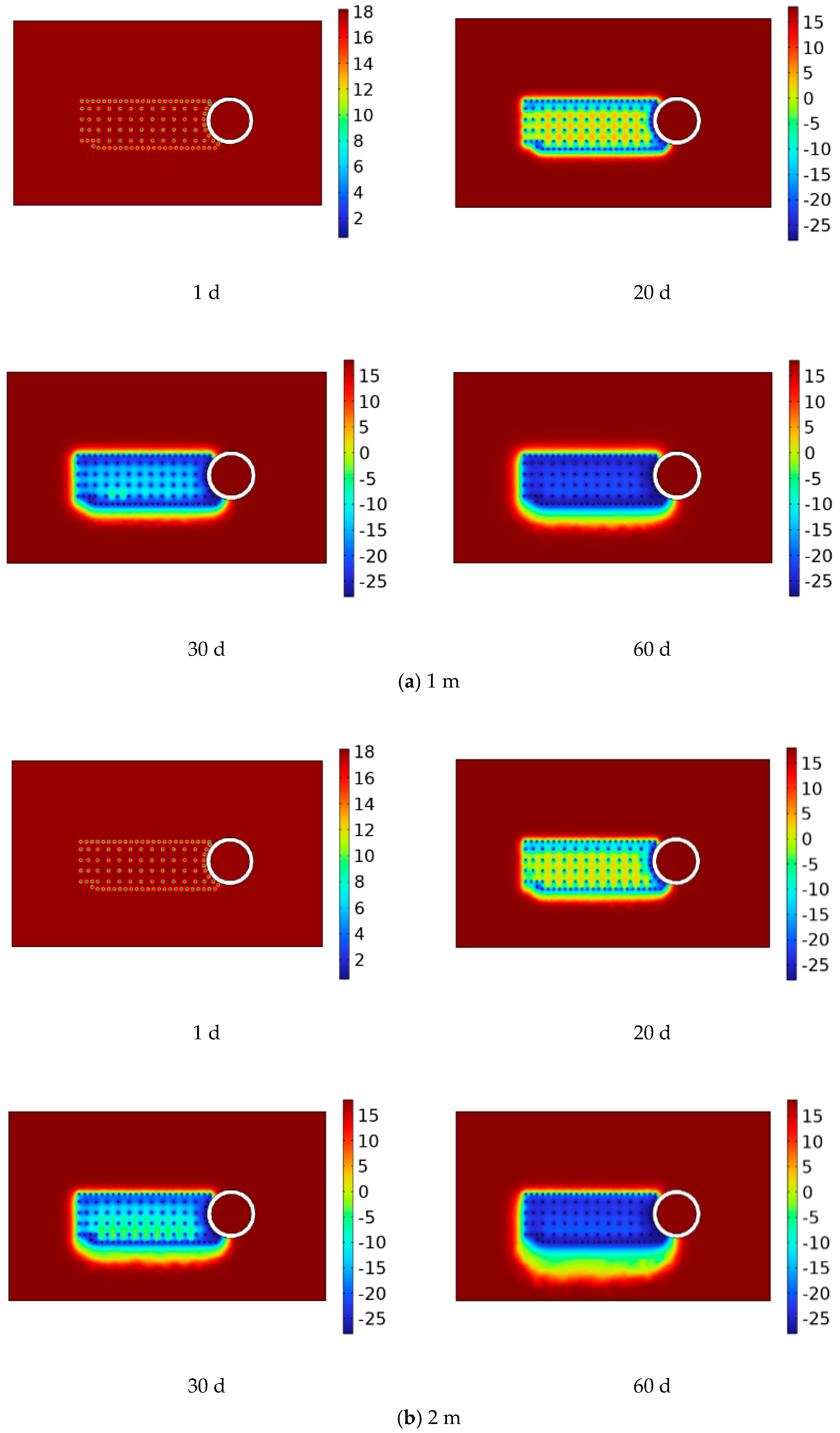
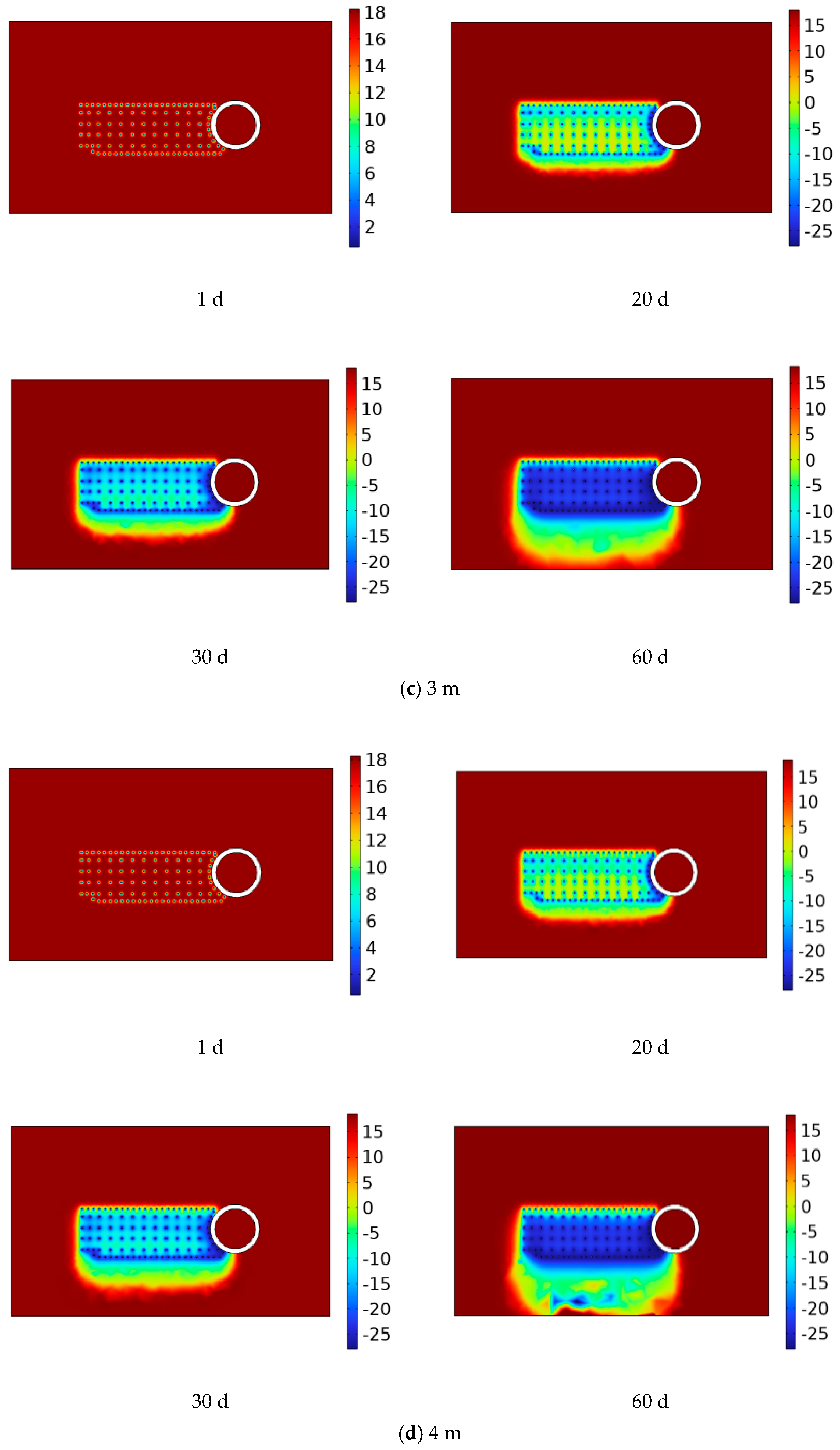
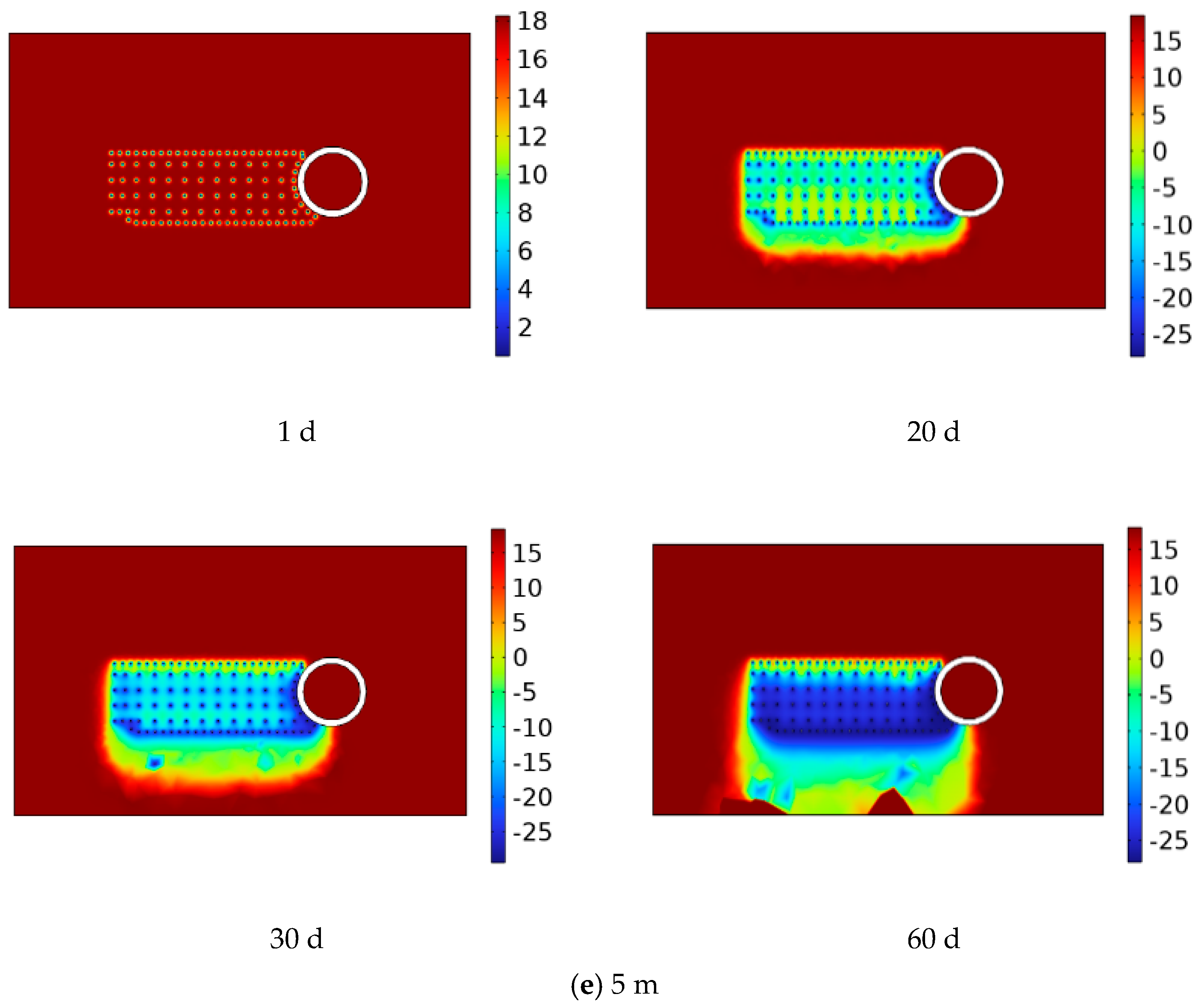
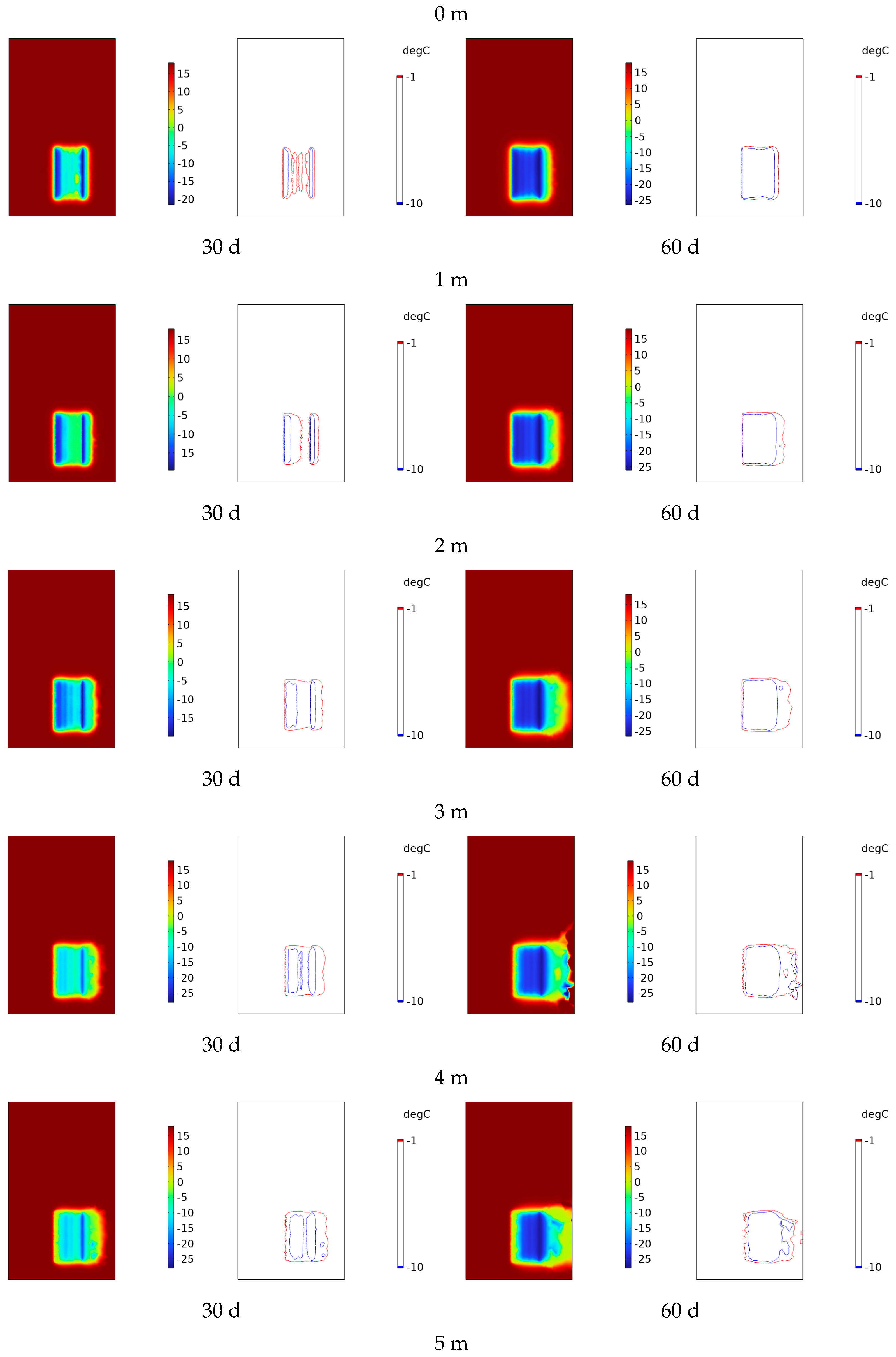
The impact of groundwater seepage on the development of permafrost barriers is a critical consideration. Under typical construction scenarios, the flow of groundwater through the porous medium is characterized by laminar flow, adhering to Darcy’s law. For the purposes of this analysis, the discussion in this study is limited to unidirectional seepage, assuming that seepage occurs exclusively at the upper and lower boundaries of the model. To elucidate the effects of varying seepage velocities on the freezing temperature field under seepage conditions, the time intervals between frozen soil curtain circles and the final thickness of the frozen soil curtain were investigated for different seepage rates. Through numerical simulations, the head differences at the upstream and downstream boundaries of the model were set to 1 m, 2 m, 3 m, 4 m, and 5 m to investigate the effect of seepage velocity changes on the freezing temperature field.
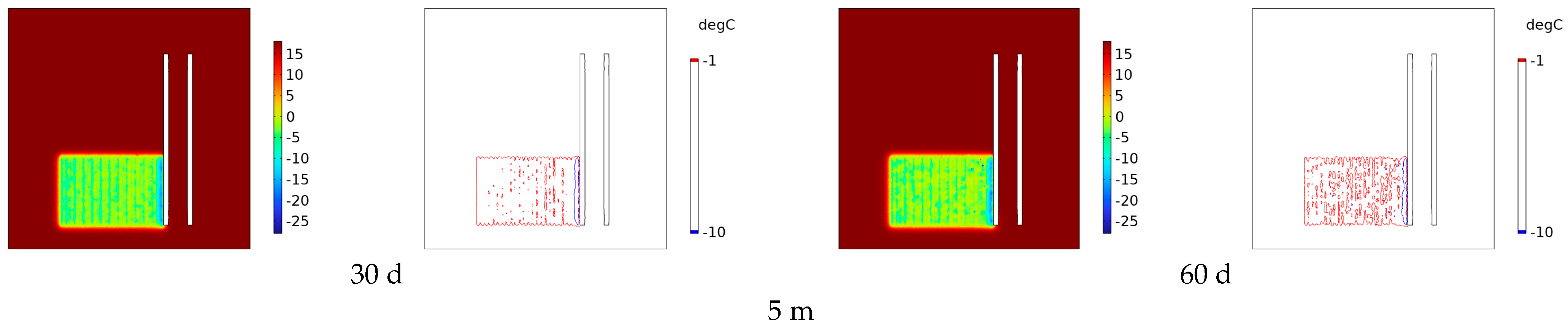
Figure 8 illustrates the changes in the freezing temperature field under various seepage velocities. For comparative analysis, temperature field cloud diagrams at 1 d, 20 d, 30 d, and 60 d were selected to examine the impact of seepage velocity on the freezing temperature field. Initially, at 1 d, the freezing tube began to generate a minimal amount of cold for different seepage velocities, which was not yet transferred to the surrounding area but was confined to the immediate vicinity of the freezing tube. At this stage, groundwater flow was horizontal and uniform, moving from high to low heads across the frozen area. By 20 d, with a head difference of 1 m, the initial outline of the frozen soil curtain started to form, and as freezing progressed, the curtain developed steadily. However, with a head difference of 2 m, the development of the frozen soil curtain was somewhat hindered, showing non-uniform growth upstream and downstream, indicating that the curtain was not yet fully closed and did not completely prevent groundwater inflow. As the freezing pipe continued to apply cold, a more stable frozen soil curtain eventually formed. A head difference of 3 m revealed that the groundwater flow influenced the freezing method’s temperature field, with the curtain’s development slowing down, particularly at the waterfront. By the 30th day, the curtain had not yet closed, and there was still a small amount of water flow within the freezing area. By the end of freezing (60 d), a very weak frozen soil curtain had formed. With head differences of 4 m and 5 m, the impact of groundwater flow on the formation of the frozen soil curtain was evident, with the curtain remaining unstable throughout the freezing period. Water flow was present in the freezing gap and through the excavation area surrounding the freezing pipe, posing a significant risk for subsequent construction excavation in actual projects. The cold produced by the freezing pipe was gradually carried downstream by the groundwater flow, leading to uneven development of the frozen soil curtain. As the seepage velocity increased, the unevenness of the curtain’s development grew, expanding the frozen area’s scope but weakening the overall freezing effect, and the curtain’s thickness gradually decreased, making it impossible to form a stable frozen soil curtain.
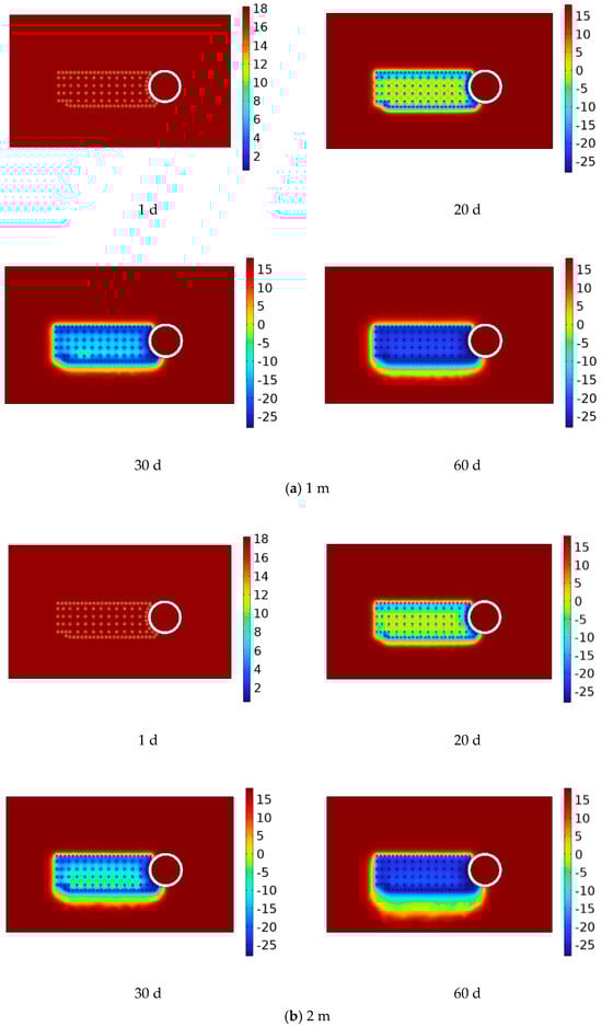

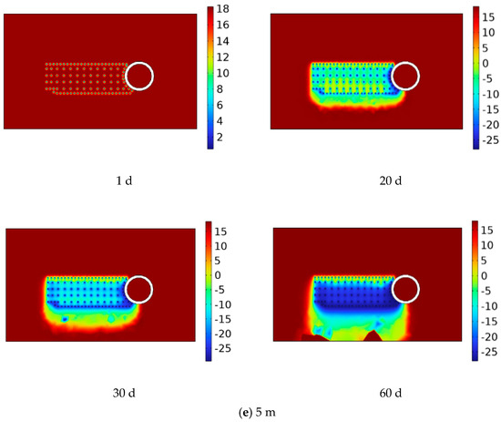
Figure 8.
Freeze optimization scheme freeze tube layout diagram.
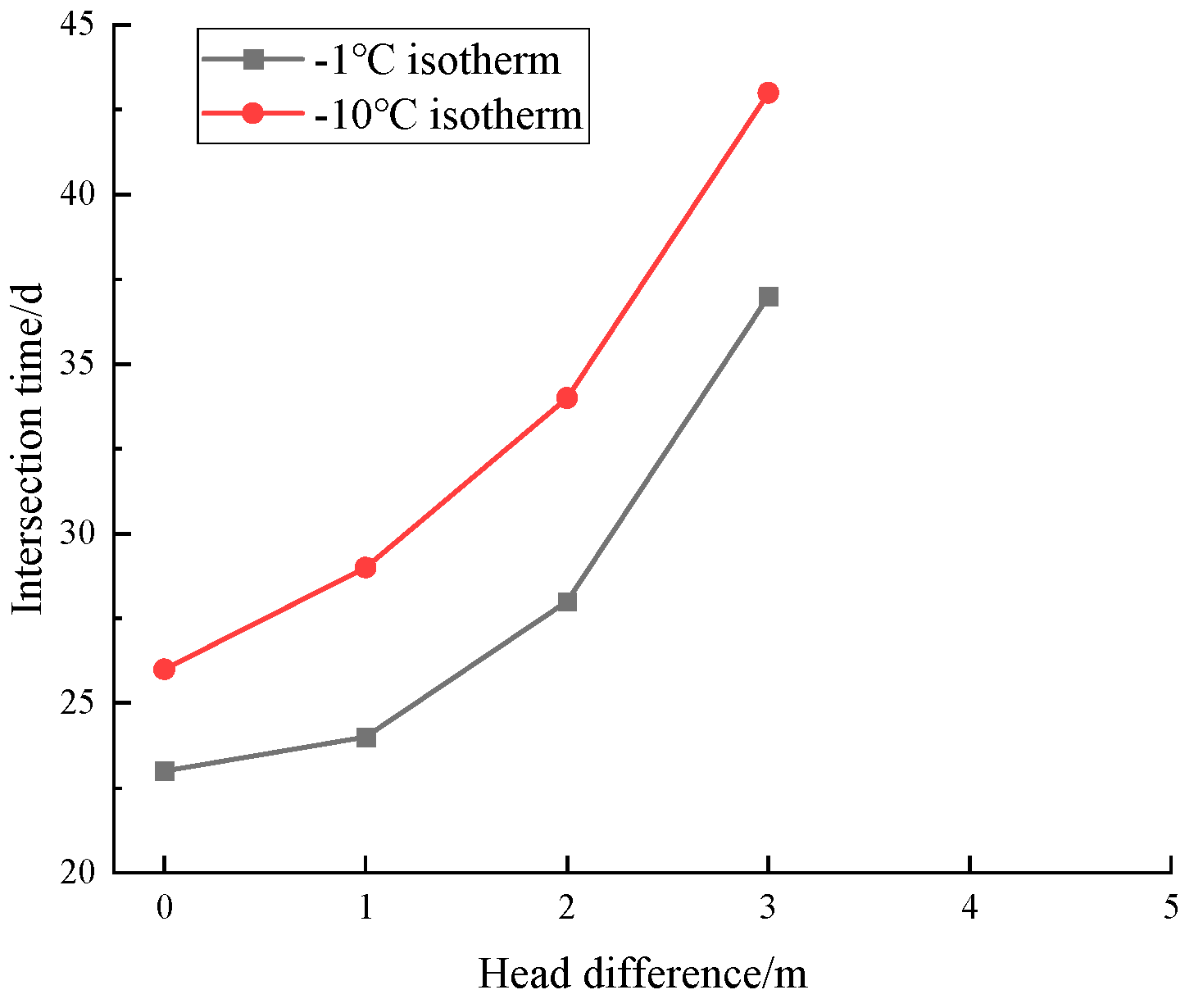
The engineering construction of permafrost curtains involves a well-developed method for measuring freezing, primarily based on two indicators: the intersection time and the specific thickness of the permafrost curtain. Figure 9 illustrates the variation in the intersection times of the −1 °C and −10 °C isotherms under different seepage velocities. As Figure 8 indicates, the intersection times of the −1 °C and −10 °C isotherms increased with an increase in seepage velocity. When the head difference surpassed 2 m, the intersection time exhibited “explosive” growth. Beyond a head difference of 3 m, the −1 °C and −10 °C isotherms did not intersect throughout the entire freezing cycle, which lasted 60 days.
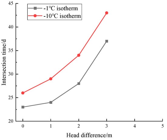
Figure 9.
Variation of intersection times of −1 °C isotherm and −10 °C isotherms with seepage rate.
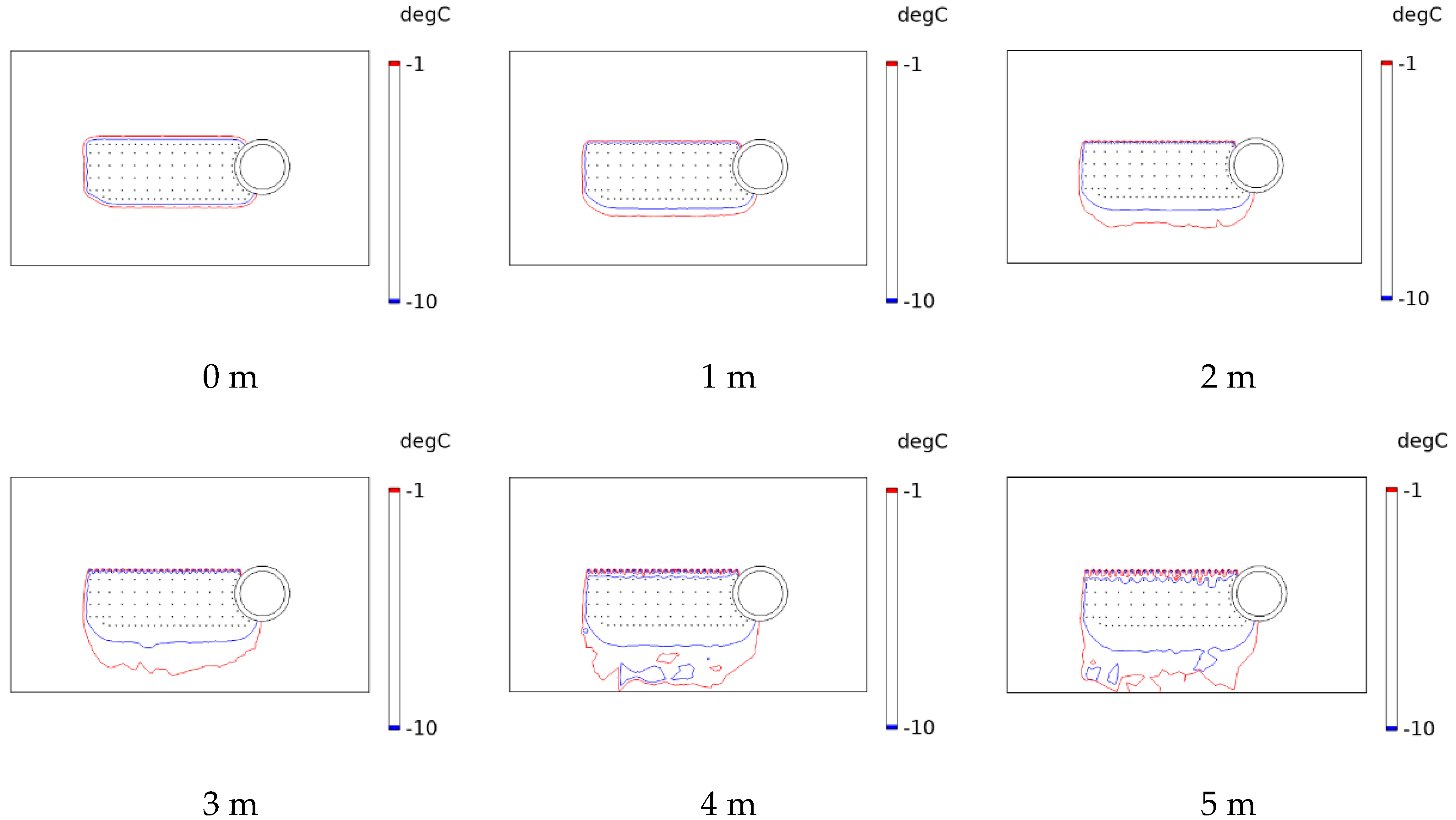
Figure 10 illustrates the development of a permafrost curtain with −1 °C and −10 °C isotherms following 30 days of active freezing. The enhanced groundwater flow rate led to a gradual reduction in the thickness of the permafrost curtain between the frozen pipes, which significantly affected upstream curtain formation. Therefore, this study focused on upstream curtain formation. Without seepage, the uniform frozen soil curtain formed by the −10 °C isotherm was approximately 2.652 m thick. When the head difference reached 1 m, the thickness of the frozen soil curtain changed minimally. However, with a head difference of 2 m, the −10 °C isotherm failed to complete the circle intersection, resulting in the upper reaches forming only a thin, weak frozen soil curtain, nearly touching the freezing tube’s edge. Beyond a head difference of 2 m, the −10 °C isotherm did not complete the circle intersection, and while the basic outline of the permafrost curtain was discernible, −10 °C isotherm–defined curtain formation was largely absent.
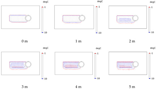
Figure 10.
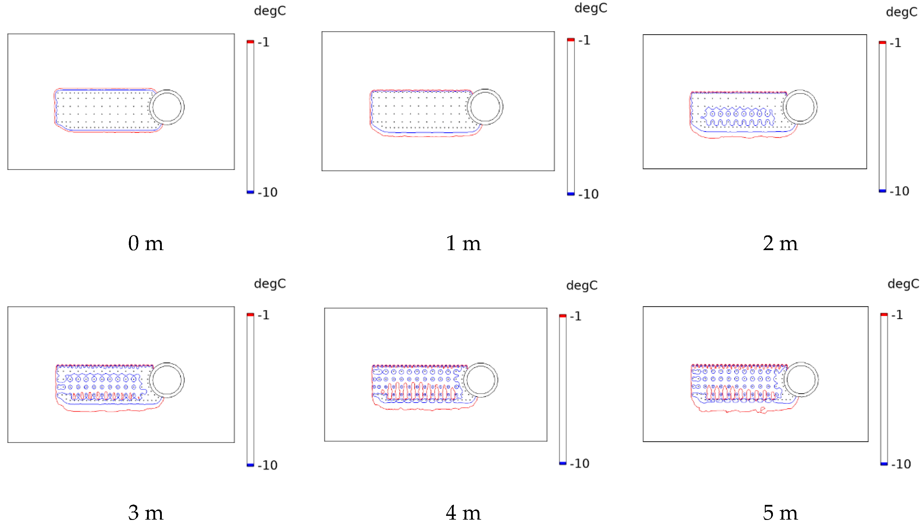
Thickness of permafrost curtain formed at 30 d of freezing for different seepage rates.
Figure 11 illustrates the permafrost curtain delineated by −1 °C and −10 °C isotherms after 60 days of active freezing. It is evident that, without any seepage, the permafrost curtain defined by the −10 °C isotherm developed most effectively, remaining stable and uniform, with a final thickness of approximately 3.023 m. It can be observed that, as the head difference increased to 1 m, the seepage velocity had a minimal impact on the permafrost curtain, resulting in a slight reduction in the upstream curtain thickness, which is about 2.893 m, a decrease of 0.13 m compared to the scenario without seepage. When the head difference reached 2 or 3 m, the permafrost curtain’s thickness was increasingly influenced by seepage velocity, with the upstream curtain formed by the −10 °C isotherm showing significant weakening, particularly close to the freezing tube, almost touching it. The degree of uniformity in the permafrost curtain, both upstream and downstream, was notably affected by the seepage velocity. As the seepage velocity surpassed 3 m, “freezing gaps” appeared on the upstream side, and the number of these gaps increased with the seepage velocity. At this point, the upstream −10 °C isotherm had not yet intersected the circle, indicating that the permafrost curtain defined by the −10 °C isotherm had not yet been fully formed.
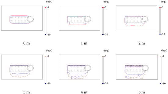
Figure 11.
Thickness of permafrost curtain formed at 60 d of freezing for different seepage rates.
4.2. X-Section Permafrost Curtain Development Law
To gain a deeper understanding of how varying seepage velocities affect the vertical freezing three-dimensional freezing temperature field, X = 15.5 m profiles were selected for 30 and 60 day analyses. The temperature field cloud diagrams and isothermal line development changes were examined. Figure 12 illustrates the pattern of change in the temperature field cloud map and isotherm map for the X = 15.5 m profile under different seepage velocities.
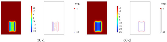

Figure 12.
Variation of temperature field cloud and isotherm maps in the X-direction cross-section.
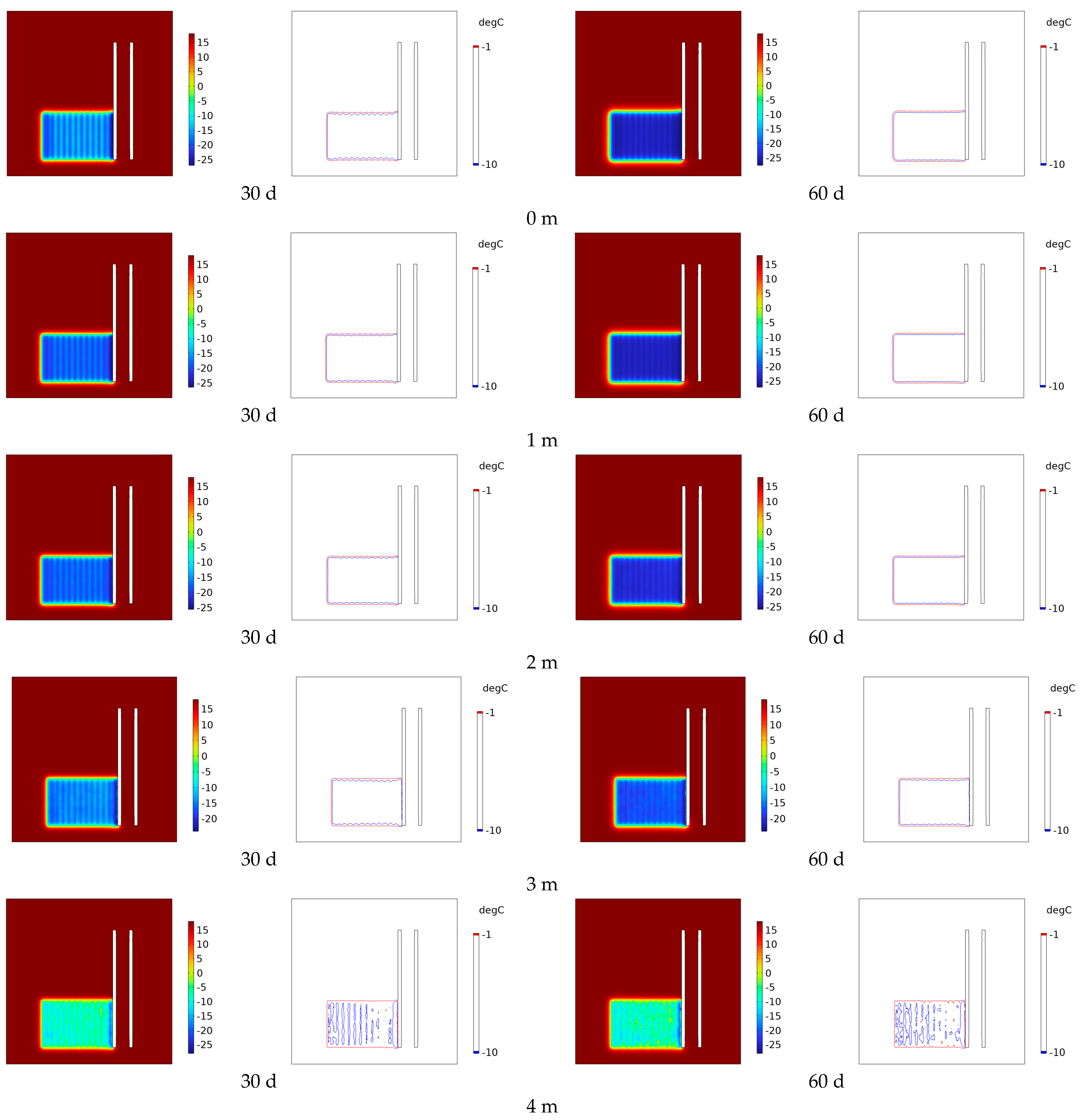
As illustrated in Figure 12, at 30 days of freezing, the permafrost curtain developed uniformly without any seepage velocity, with the isotherms measured upstream and downstream completing their intersection circle first due to the significant number of freezing pipes upstream and downstream. As the seepage velocity increased, driven by the groundwater flow upstream, the cold generated by the upstream freezing pipe was continuously transported downstream, leading to a substantial accumulation of cold within the internal freezing zone. When the head difference reached 3 m, the −1 °C isotherm had completed its intersection circle, yet the development of the frozen curtain was uneven; this inhomogeneity increased with the seepage velocity. By 60 days of freezing, in the absence of seepage, the overall development of the permafrost curtain was stable and uniform. With increasing seepage velocity, the development of the frozen curtain on both the upstream and downstream sides became uneven. The thickness of the frozen curtain on the upstream side gradually decreased and approached the freezing pipe, while the downstream side exhibited a “tailing” phenomenon, with the freezing range expanding. When the head difference reached 4 m, the −1 °C and −10 °C isotherms on the downstream side did not intersect, failing to reach the freezing temperature. The unevenness of the frozen curtain development increased with the seepage velocity, which both expanded some frozen areas and diminished the overall freezing effect.
4.3. Y-Section Permafrost Curtain Development Law
To gain a better understanding of the variations in seepage velocity within the vertical freezing three-dimensional freezing temperature field, a deliberate choice was made to select a location near the upstream side in the Y direction. Consequently, the profile at Y = 16.2 m was chosen for analysis of temperature field cloud diagrams and evolution of isotherms over 30 and 60 days. Figure 13 illustrates the temperature field cloud diagrams and the changes in isotherms for different seepage velocities at this profile.

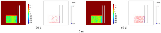
Figure 13.
Variation of temperature field cloud and isotherm maps in the Y-direction cross-section.
As illustrated in Figure 13, without considering seepage velocity, the frozen soil curtain developed uniformly over the initial 30 days of freezing. This uniform development was attributed to the equal progression of the frozen soil curtain upstream and downstream. At this stage, both the −1 °C and −10 °C isotherms had completed their intersection with the circle. As the freezing time progressed, the frozen soil curtain continued to develop steadily and thicken. When the head difference increased, the profile at Y = 15.5 experienced less influence from seepage velocity for head differences of 1 m, 2 m, and 3 m. However, at a head difference of 4 m, the −10 °C isotherms were notably present within the internal freezing area at 30 days of freezing. By this time, the −1 °C isotherms had completed their inter-circle. Further freezing to 60 days revealed that the −10 °C isotherms had not completed their inter-circle. When the head difference reached 5 m, the −1 °C isotherms within the frozen area had not completed their inter-circle, suggesting that a small portion of the internal frozen area had not reached the freezing temperature.
5. Analysis of Pathway Observation Points
5.1. Temperature Comparison of Upstream and Downstream Symmetry Points Under Seepage Conditions
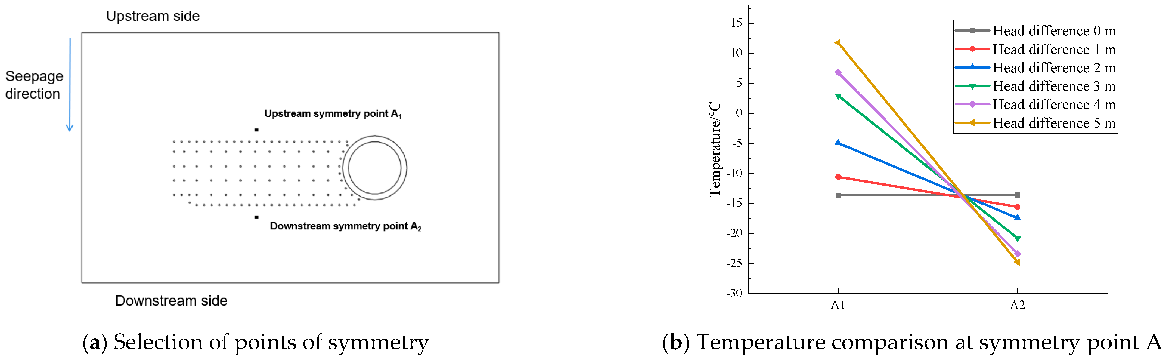
To accurately investigate the impact of groundwater flow velocity on the freezing process of permafrost curtains, it is evident from the previous subsection that the seepage conditions upstream and downstream of the curtain exhibit non-uniformity. Consequently, symmetry points were established at distances of 2 m from the outermost edge of the freezing pipes, both upstream and downstream. These points are denoted as A1 and A2, as illustrated in Figure 14a.
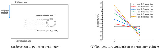
Figure 14.
Temperature variations at different locations of symmetry points at different percolation rates.
As illustrated in Figure 14b, comparison of temperatures at the observed points relative to the symmetric point A under various seepage velocities indicated that the temperature variations upstream and downstream of point A were minimal and nearly symmetrical in the absence of seepage. As the seepage velocity increased, the inclination angle of the line connecting these points gradually increased. At a seepage velocity of 2 m, the temperature at symmetric point A1 was approximately −4.96 °C, which is a 10 °C difference from the no-seepage condition due to the groundwater flow continuously transferring coldness from upstream to downstream. When the seepage rate reached 3 m, the temperature at the symmetry point A1 remained above freezing, at about 2.96 °C. In summary, it can be concluded that the groundwater flow rate exerts a discernible impact on the temperatures of the upstream and downstream symmetry points, with the temperature difference between these points increasing as the seepage rate increases.
5.2. Analysis of Pathway Observation Points
5.2.1. Path Selection
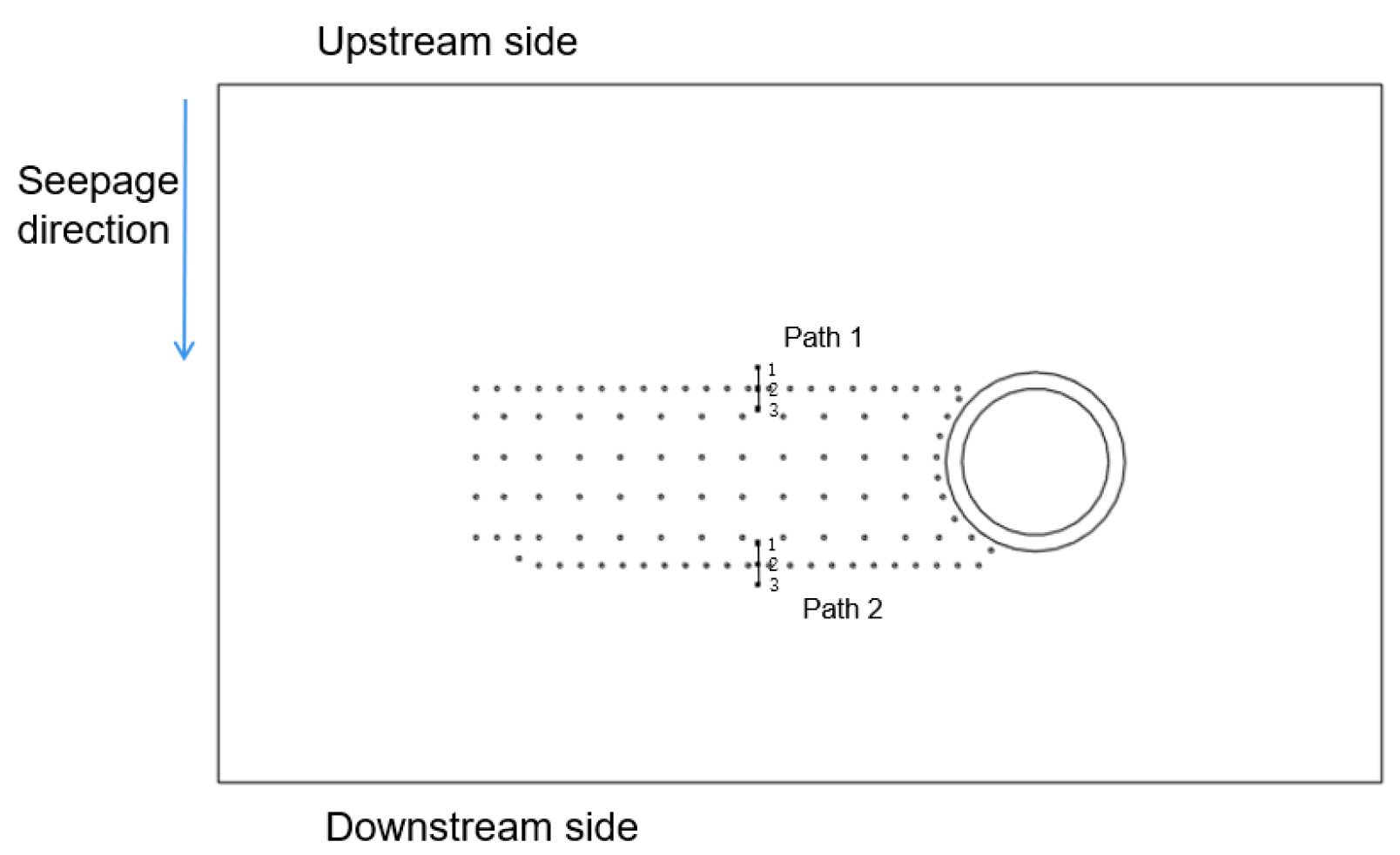
To better understand the evolution of the temperature field, two paths were established within the model: Path 1 and Path 2. Path 1 was situated in the upstream freezing region, while Path 2 was located in the downstream freezing region. For each path, an observation point was set at every meter, resulting in a total of three observation points. The observation path diagram is depicted in Figure 15. The distinct paths within the model clearly illustrate the cooling behavior of the temperature field, offering valuable insights for future construction. To ensure the accuracy of the numerical analysis of the temperature field for the freezing method, the results were compared with numerical simulations based on numerous on-site measurements. The relevant data obtained largely corroborated these findings, as detailed in the related literature [27,28].

Figure 15.
Path diagram.
5.2.2. Analysis of Cooling Patterns at Temperature Observation Points
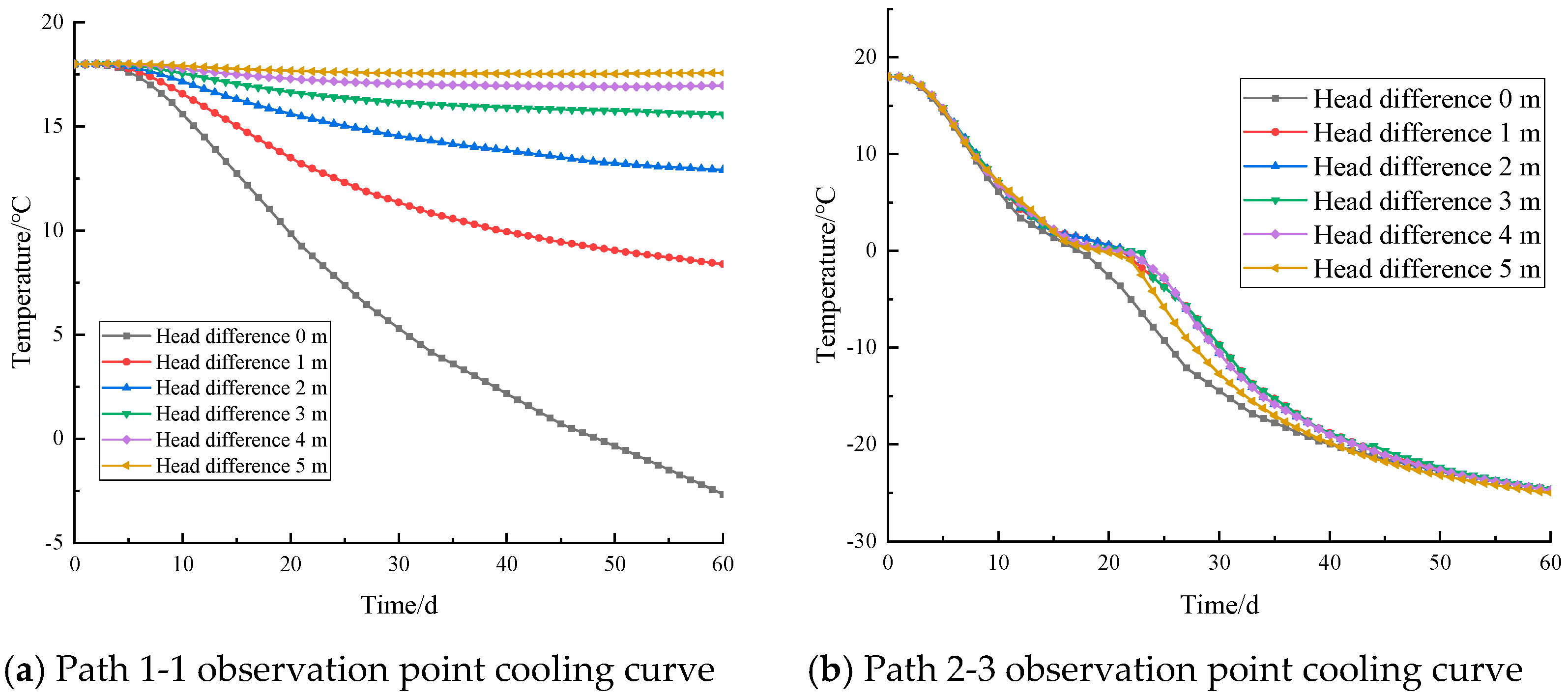
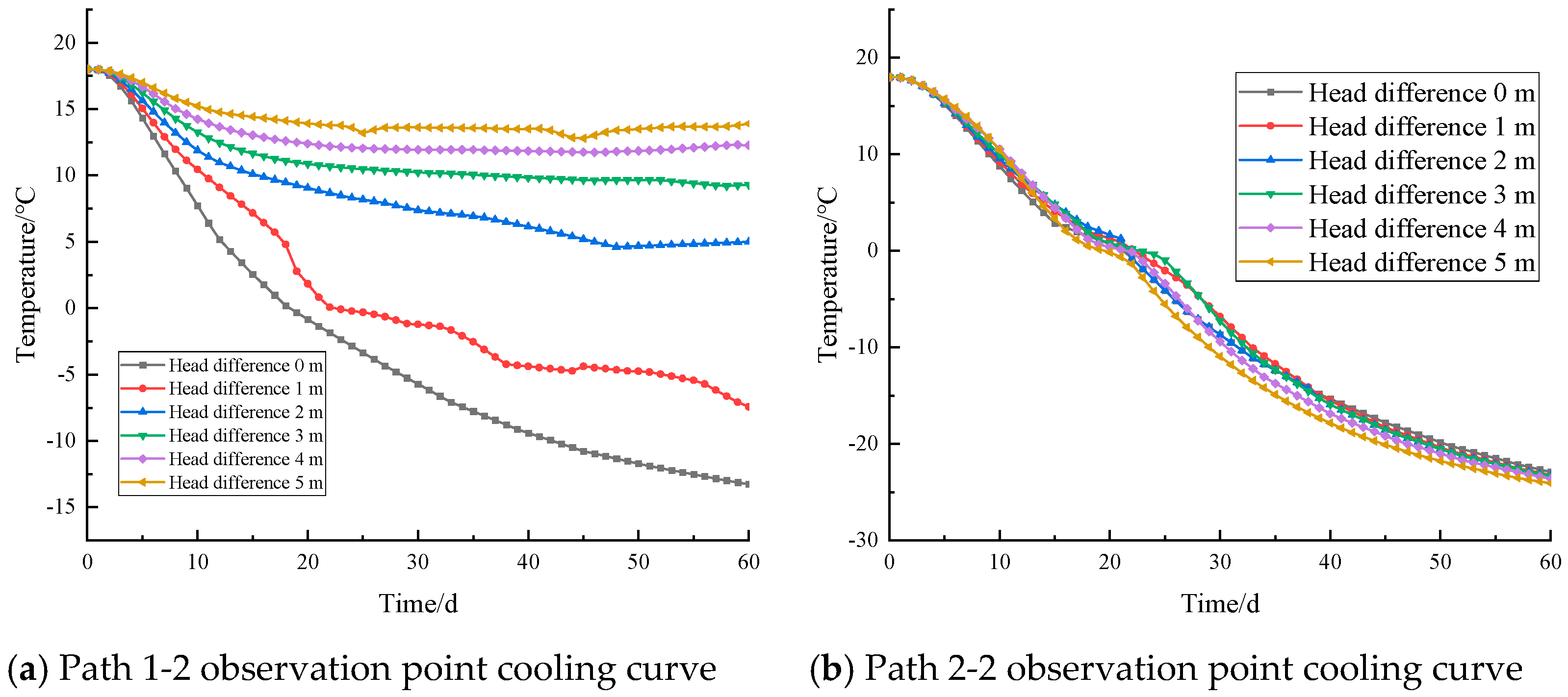
To thoroughly investigate the impact of subsurface flow velocity on the freezing temperature field, four temperature measurement points, Path 1-y (y = 1, 2) and Path 2-y (y = 2, 3), were selected based on the paths depicted in Figure 15 to analyze the cooling curves under various seepage velocities.
Figure 16 presents the cooling curves of the temperature measurement points on the upstream and downstream sides, respectively. The impact of different seepage velocities on temperature measurement points at various locations was evident, with the temperature observation point Path 1-1, situated upstream of the freezing region, being particularly sensitive to seepage velocity. Given that Path 1-1-was is located further upstream from the freezing tube, freezing temperature was only reached in the absence of flow. As seepage velocity increased, all temperature observation points remained above 0 °C, and the formation of a frozen soil curtain also varied with the increase in groundwater flow rate. This is attributed to the fact that a higher groundwater seepage rate continuously transports the cold generated by the upstream freezing pipe downstream, resulting in higher temperatures at these observation points after 60 days of active freezing. Conversely, temperature measurement points located downstream within the freezing area were less affected by groundwater flow. The temperature of the Path 2-2 temperature measurement point showed little variation with different groundwater flow rates, and the cooling curve trend remained consistent. This is due to the fact that groundwater continuously carries the cold from the upstream freezing pipe downstream, ensuring sufficient cold to reduce the soil body temperature.

Figure 16.
Effect of different seepage rates on different observation points.
The temperature measurement points between the freezing pipes at various locations exhibited distinct cooling curves, as illustrated in Figure 17. It is evident that the flow rate of groundwater exerted a minimal impact on the temperature of Path 2-3. The cooling curves of the temperature measurement points under different flow rates nearly coincided, indicating low sensitivity to variations in seepage velocity. Conversely, the temperature measurement points of Path 1-2 were more responsive to changes in seepage velocity. Prior to 20 days before freezing, the cooling curves of the temperature measurement points showed a decreasing amplitude when the flow rate exceeded 1 m. At a flow rate of 1 m, the temperatures of the temperature measurement points remained above 0 °C and had not yet reached the freezing point.
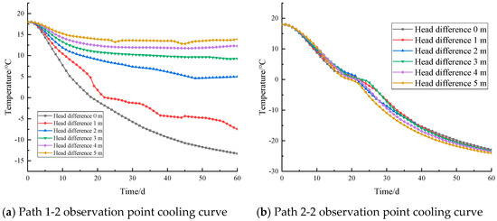
Figure 17.
Sensitivity analysis of different seepage rates to cooling at different observation points.
6. Conclusions
In this study, the engineering background is tunnel collapse repair, where vertical freezing is employed to reinforce the soil body at the site of the collapse. The finite element software COMSOL was utilized to construct a three-dimensional water–heat coupling model, enabling detailed investigation of the temperature field within the collapsed soil body. The study concludes with the following findings.
(1) In the absence of seepage, the permafrost curtain evolved stably and uniformly across the frozen zone. As evident from the isotherm chart, the permafrost curtains in the upstream and downstream regions exhibited instability and non-uniformity in the presence of seepage. The degree of non-uniformity in these curtains increased significantly with an escalating seepage rate. The temperature disparity between the upstream and downstream areas could be discerned through the temperatures of the symmetry points for each region.
(2) The presence of permafrost curtains significantly altered the groundwater flow dynamics. Analysis of the cloud diagrams revealed that the introduction of permafrost curtains caused the groundwater to divert around these barriers, transitioning from a parallel flow pattern to one that bypassed the curtains. Once a closed permafrost curtain was established, groundwater flow was effectively blocked in the areas encircled by the curtains, leading to the development of a “trailing tail” downstream of the frozen zone. This phenomenon intensified as the groundwater carried cold from the upstream freezing pipes to the downstream regions, resulting in the formation of a “trailing tail” at the downstream edge of the frozen area. Moreover, as the groundwater seepage rate increased, the size of the “trailing tail” also expanded.
(3) The intersection time of isotherms was a critical indicator for assessing the evolution of a permafrost curtain. Specifically, the −1 °C and −10 °C isotherms exhibited an increase in intersection time with a rise in seepage velocity. Notably, when the head difference surpassed 2 m, the intersection time of the −1 °C and −10 °C isotherms experienced “explosive” growth. Conversely, at a head difference of 3 m, the −1 °C and −10 °C isotherms did not intersect throughout the entire freezing cycle duration of 60 days.
(4) Enhancement of seepage velocity led to a reduction in the thickness of the permafrost curtain, creating a vulnerable zone between the frozen pipes. The increase in groundwater flow rate exerted a more pronounced effect on the freezing process upstream, with the cooling curves of temperature measurement points upstream of the freezing area exhibiting heightened sensitivity to variations in groundwater flow rate as it rose. Conversely, the cooling curves of temperature measurement points downstream of the freezing area were nearly identical and showed less sensitivity to changes in groundwater flow rate. The influence of groundwater flow rate on the frozen soil curtain was observed to be greater upstream compared to downstream.
As the artificial bottom freezing method is widely used in tunnel reinforcement work, some of the conclusions drawn in this study have some similarities with other studies, which further validates the correctness of the conclusions drawn in this paper. However, this study was based on the reinforcement and rehabilitation of collapsed tunnels and adopted a vertical freezing scheme, which is a special feature of this study and different from other studies. In the next study, the development of the frozen curtain will be further explored, mainly for field measurements and model tests.
Author Contributions
Conceptualization, H.G. and J.H.; methodology, H.G., J.H., T.Y. and X.S.; validation, J.H., H.G., J.Z. and L.H.; data curation, H.G.; writing—original draft preparation, H.G. and J.H.; writing—review and editing, J.H., H.G. and T.Y.; funding acquisition, J.H. and J.Z. All authors have read and agreed to the published version of the manuscript.
Funding
The High Technology Direction Project of the Key Research and Development Science and Technology of Hainan Province, China (Grant No. ZDYF2024GXJS001); the Hainan University Collaborative Innovation Center Project (Grant No. XTCX2022STB09); the Key Research and Development Projects of the Haikou Science and Technology Plan for the Year 2023 (2023-012); and the Hainan Provincial Innovation Foundation for Postgraduate (Qhyb2023-117).
Institutional Review Board Statement
Not applicable.
Informed Consent Statement
Not applicable.
Data Availability Statement
The original contributions presented in the study are included in the article. Further inquiries can be directed to the corresponding author.
Acknowledgments
I would like to express my sincerest gratitude for the support and assistance I received from Haizuo Zhou in completing this manuscript. I would like to thank Zhou for his careful guidance and constant encouragement during my research.
Conflicts of Interest
Author Lei Huang was employed by the company Shandong Jiayu Engineering Construction Co., Ltd. Author Xinming Shang was employed by the company Junchi Engineering Co., Ltd. The remaining authors declare that the research was conducted in the absence of any commercial or financial relationships that could be construed as a potential conflict of interest.
References
- Zhan, Y.; Lu, Z.; Yao, H. Numerical analysis of thermo-hydro-mechanical coupling of diversion tunnels in a seasonally frozen region. J. Cold Reg. Eng. 2020, 34, 04020018. [Google Scholar] [CrossRef]
- Williams, R.J.; Alsahly, M.A.; Meschke, G. Computational modelling of artificial ground freezing in mechanized tunnelling. In Expanding Underground-Knowledge and Passion to Make a Positive Impact on the World; CRC Press: Boca Raton, FL, USA, 2023; pp. 1510–1514. [Google Scholar]
- Jin, H.; Lee, J.; Ryu, B.H.; Go, G.H. Experimental and numerical study on hydro-thermal behaviour of artificial freezing system with water flow. J. Korean Geotech. Soc. 2020, 36, 17–25. [Google Scholar]
- Zhelnin, M.; Kostina, A.; Plekhov, O.; Panteleev, I.; Levin, L. Numerical simulation of soil stability during artificial freezing. Procedia Struct. Integr. 2019, 17, 316–323. [Google Scholar] [CrossRef]
- Zhou, J.; Li, Z.; Wan, P.; Tang, Y.; Zhao, W. Effects of seepage in clay-sand composite strata on artificial ground freezing and surrounding engineering environment. Chin. J. Geotech. Eng. 2021, 43, 471–480. [Google Scholar]
- Mauro, A.; Normino, G.; Cavuoto, F.; Marotta, P.; Massarotti, N. Modeling artificial ground freezing for construction of two tunnels of a metro station in Napoli (Italy). Energies 2020, 13, 1272. [Google Scholar] [CrossRef]
- Niu, Y.; Hong, Z.Q.; Zhang, J.; Han, L. Frozen curtain characteristics during excavation of submerged shallow tunnel using Freeze-Sealing Pipe-Roof method. Res. Cold Arid. Reg. 2022, 14, 267–273. [Google Scholar] [CrossRef]
- Hong, Z.; Zhang, J.; Han, L.; Wu, Y. Numerical Study on Water Sealing Effect of Freeze-Sealing Pipe-Roof Method Applied in Underwater Shallow-Buried Tunnel. Front. Phys. 2022, 9, 794374. [Google Scholar] [CrossRef]
- Cui, Z.D.; Zhang, L.J.; Xu, C. Numerical simulation of freezing temperature field and frost heave deformation for deep foundation pit by AGF. Cold Reg. Sci. Technol. 2023, 213, 103908. [Google Scholar] [CrossRef]
- Alzoubi, M.A.; Xu, M.; Hassani, F.P.; Poncet, S.; Sasmito, A.P. Artificial ground freezing: A review of thermal and hydraulic aspects. Tunn. Undergr. Space Technol. 2020, 104, 103534. [Google Scholar] [CrossRef]
- Pang, C.; Cai, H.; Hong, R.; Li, M.; Yang, Z. Evolution law of three-dimensional non-uniform temperature field of tunnel construction using local horizontal freezing technique. Appl. Sci. 2022, 12, 8093. [Google Scholar] [CrossRef]
- Afshani, A.; Akagi, H. Artificial ground freezing application in shield tunneling. Jpn. Geotech. Soc. Spec. Publ. 2015, 3, 71–75. [Google Scholar] [CrossRef]
- Li, M.; Cai, H.; Liu, Z.; Pang, C.; Hong, R. Research on frost heaving distribution of seepage stratum in tunnel construction using horizontal freezing technique. Appl. Sci. 2022, 12, 11696. [Google Scholar] [CrossRef]
- Zhang, C.; Yang, W.; Qi, J.; Zhang, T. Analytic computation on the forcible thawing temperature field formed by a single heat transfer pipe with unsteady outer surface temperature. J. Coal Sci. Eng. 2012, 18, 18–24. [Google Scholar] [CrossRef]
- Zhou, X.; Jiang, G.; Li, F.; Gao, W.; Han, Y.; Wu, T.; Ma, W. Comprehensive review of artificial ground freezing applications to urban tunnel and underground space engineering in China in the last 20 years. J. Cold Reg. Eng. 2022, 36, 04022002. [Google Scholar] [CrossRef]
- Kang, Y.; Hou, C.; Li, K.; Liu, B.; Sang, H. Evolution of temperature field and frozen wall in sandy cobble stratum using LN2 freezing method. Appl. Therm. Eng. 2021, 185, 116334. [Google Scholar] [CrossRef]
- Liu, R.; Zhang, Q.; Hu, X.; Tan, L. Application of Horizontal Ground Freezing Method in Shanghai Metro Rehabilitation Project. J. Anhui Univ. Archit. Technol. (Nat. Sci. Ed.) 2008, 3, 21–25. [Google Scholar]
- Hu, X.; Long, L. Submarine Shield Repair Freeze Reinforcement Technology. J. Undergr. Space Eng. 2010, 6, 537–542. [Google Scholar]
- Hao, M.; Shi, Z. Application of Freezing Method in the Rehabilitation of River Bottom Intake Tunnels. Well Constr. Technol. 2014, 35, 12–16. [Google Scholar] [CrossRef]
- Xiao, Z.; Hu, X.; Zhang, Q. Design of Freezing Method in Subway Rehabilitation Works. J. Geotech. Eng. 2006, 1716–1719. [Google Scholar]
- Chu, Y.; Zhu, B.; Zhang, Y. Application of Freezing Method in Rehabilitation Works of Cross River Tunnel. Tunn. Constr. 2010, 30, 596–599. [Google Scholar]
- Xiao, Z.; Hu, X.; Zhang, Q. Application of four-row local freezing method in Shanghai metro repair project. Geotechnics 2006, 27, 300–304. [Google Scholar] [CrossRef]
- Fu, Y.; Hu, J.; Wu, Y. Finite element study on temperature field of subway connection aisle construction via artificial ground freezing method. Cold Reg. Sci. Technol. 2021, 189, 103327. [Google Scholar] [CrossRef]
- Liu, P.; Hu, J.; Dong, Q.; Chen, Y. Studying the Freezing Law of Reinforcement by Using the Artificial Ground Freezing Method in Shallow Buried Tunnels. Appl. Sci. 2024, 14, 7106. [Google Scholar] [CrossRef]
- Hu, J. Experimental Study on Freezing Temperature and Mechanical Properties of Soil Before and After Cement Improvement. Railw. Constr. 2013, 18, 156–159. [Google Scholar]
- Jun, H.; Ping, Y.; Zhao-wen, D.; Rong, C. Study on numerical simulation of cup-shaped horizontal freezing reinforcement project near shield launching. In Proceedings of the International Conference on Electric Technology and Civil Engineering (ICETCE), Lushan, China, 22–24 April 2011; pp. 5522–5525. [Google Scholar]
- Liu, W.B. Research on Freezing and Reinforcement Technology of Large-Diameter Shield Tunneling in Heyan Road Cross-River Channel in Nanjing; Hainan University: Haikou, China, 2021. [Google Scholar]
- Wu, Y.W. Research on the Evolution of Construction Temperature Field of Freezing Method of Dongbin Section of Nanning Metro; Hainan University: Haikou, China, 2019. [Google Scholar]


Disclaimer/Publisher’s Note: The statements, opinions and data contained in all publications are solely those of the individual author(s) and contributor(s) and not of MDPI and/or the editor(s). MDPI and/or the editor(s) disclaim responsibility for any injury to people or property resulting from any ideas, methods, instructions or products referred to in the content. |
© 2025 by the authors. Licensee MDPI, Basel, Switzerland. This article is an open access article distributed under the terms and conditions of the Creative Commons Attribution (CC BY) license (https://creativecommons.org/licenses/by/4.0/).