Experimental and Theoretical Evaluation of Incident Solar Irradiance on Photovoltaic Power Plants Under Real Operating Conditions: Fixed Tilt Angle System vs. Horizontal Single-Axis Tracker

Abstract

The aim of this paper was to delve deeper into the nuances of incident solar irradiance on the photovoltaic field of a fixed tilt angle system versus a horizontal single-axis tracker. The fixed tilt angle system was used as a baseline for comparison. Three assessment indicators were analysed (annual energy gain ($AEG$), monthly energy gain ($MEG$), daily energy gain ($DEG$)). The procedure used comprised the following steps: (i) choice of solar irradiance estimation model; (ii) theoretical study; (iii) study under real operating conditions—for this purpose, an experimental setup was used; and (iv) comparison of these studies. The experimental setup was installed at the Department of Electrical Engineering of the University of Oviedo (Gijón, Spain) (latitude $43°{31}^{\prime }{22}^{″}$ N, longitude $05°{43}^{\prime }{07}^{″}$ W, elevation 28 (m) above sea level). Gijón is characterised by a temperate oceanic climate typical of Spain’s Atlantic coast, with cool summers and wet and mostly mild winters. The code assigned to Gijón under the Köppen climate classification is $C_{fb}$. The horizontal single-axis trackers that comprise photovoltaic power plants have three operating modes (Scenario 1). Some studies consider a unique mode of operation from sunrise to sunset (Scenario 2). The following conclusions can be drawn from the results obtained: (i) although the results obtained in the theoretical study and in the study under real operating conditions were different, a trend can be seen in the results; for example, the $AEG$ obtained was approximately $13\%$ and $8.5\%$ in the theoretical study and in the real study, respectively, in Scenario 1 and approximately $18\%$ and $10.5\%$, respectively, in Scenario 2; Scenario 2 obtained higher results than Scenario 1 in all the assessment indicators; but it must be considered that Scenario 1 is the real mode of operation; (ii) from March to September, the horizontal single-axis tracker generates more electrical energy; as this period contains the months of greatest solar irradiance, the horizontal single-axis tracker performs better annually; considering the theoretical study and Scenario 1, the highest value of $MEG$ was in June ($43\%$) and the lowest was in December ($-29\%$); when the study was considered under real operating conditions, the highest result was in July ($30\%$) and the lowest was in December ($-24\%$); (iii) on the days between 70 and 277 in Scenario 1, the horizontal single-axis tracker generated more electrical energy; on the other days the opposite occurred; taking into account the theoretical study, the highest and lowest $DEG$ values were $43\%$ and $-30\%$, respectively; when the study was considered under real operating conditions, the highest and lowest $DEG$ values were $58\%$ and $-47\%$, respectively.

1. Introduction

Today’s societies are highly dependent on electricity. It has been estimated that electricity accounted for $20\%$ of global final energy consumption in 2023 [1] and that its share will be $30\%$ in 2030 [1]. This increase is justified by the global decarbonisation targets set out in the Net Zero Emissions Scenario for 2050 [2]. In the European Union ($EU$), strategies for the decarbonisation of the industrial sector promote the electrification of processes [3]. Given the increase in electricity consumption, it is also necessary to decarbonise the electricity sector [4].

Three sectors worldwide are the big consumers of final energy. In 2022, these sectors were [5] industry ($30.41\%$), the transport sector ($27.81\%$), and the household sector ($20.30\%$). Many industrial processes are highly dependent on electricity, such as (i) energy-intensive industries (steel, paper industries, etc.) and (ii) other industries (construction, textile, etc.). In addition, electricity is essential in the household sector, as it is used in cookers and ovens, refrigerators, washing machines and dishwashers, space heating, water heating, etc. The trend is for electricity consumption to increase with the introduction of new technologies, such as electric vehicles and hydrogen generation. A report by the International Energy Agency [6] estimates that electricity consumption in 2050 will be as follows: (i) 10,196.56 (TWh) in intensive industries, (ii) $9434.89$ (TWh) in other industries, (iii) $9385.75$ (TWh) in appliances and cooking, (iv) $7862.41$ (TWh) in cooling and heating (space heating, water heating, etc.), (v) $8476.66$ (TWh) in hydrogen production, and (vi) $4078.62$ (TWh) in light-duty vehicles.

The negative aspect of this high consumption of electricity is that its generation is considered the largest source of carbon dioxide ($C{O}_2$) emissions worldwide [1]. The direct relationship between greenhouse gas emissions and the use of fossil fuels has been the subject of a multitude of investigations [7]. Therefore, it is necessary for the energy sector to make the transition to net zero emissions. This transition is based on the expansion of the use of renewable energy sources, such as solar and wind energy.

Although the value of solar irradiance received in different locations around the world is not the same and, therefore, the profitability of the project is different, $PV$ technology can be considered an adequate solution for reducing $C{O}_2$ emissions from the electricity sector. Its characteristics, such as ease of installation, low maintenance, and scalability, place it at the top of the list of solutions to the environmental problems associated with the electricity sector.

The use of photovoltaic energy is beneficial for the environment [8], but, due to the inherent characteristics of its procedure of generating electrical energy, this energy is technically different from conventional electrical energy production plants, as its production is not controlled by the plant operator. Therefore, the penetration of this type of plant into the electricity market can pose challenges for the operation of electricity grids [9].

Intermittency and uncertainty in the energy production of a $PV$ power plant are two negative aspects of this technology [10], as it depends on meteorological phenomena that are exogenous to the energy production process. Intermittency encompasses hourly fluctuations in energy production caused by changes in the weather [11]. On the other hand, uncertainty is caused by deviations in energy production from the forecasts of the plant operator [12], who cannot predict the weather with any degree of accuracy. Therefore, this dependence of $PV$ power plants on meteorological factors raises problems of stability in the electricity grid [13]. To reduce these problems, predictive techniques have been developed to reduce uncertainty [14]. On the other hand, energy storage can eliminate the intermittency of a $PV$ power plant [15].

Stable energy production using $PV$ power plants requires energy storage to buffer supply imbalances. If short-term electricity storage is required, batteries are the solution, as they are highly efficient and flexible [16]. On the other hand, if long-term storage is required, hydrogen-based systems are more effective [17].

The problems indicated above do not reduce the importance of $PV$ power plants in the electrical system. The energy production of a $PV$ power plant is a fundamental factor in its design. Therefore, it is necessary to analyse the $PV$ module mounting systems, as energy production depends on this choice. $PV$ module mounting systems can be classified according to the presence of moving parts in their structure. Therefore, the first classification will be whether the mounting system has moving parts or not. If it has no moving parts, they are called fixed tilt angle systems. If they have moving parts, they can be classified according to the number of rotation movements [18]: dual-axis trackers and single-axis trackers. The latter can be classified, in turn, into horizontal single-axis trackers, vertical single-axis trackers, and polar single-axis trackers. The horizontal single-axis tracker is the most widely used of the three [19]. The presence of moving parts in the structure of the mounting system will be a fundamental aspect in its analysis.

As will be shown in detail in Section 2, a key aspect in the design phase of a $PV$ power plant is the choice of $PV$ module mounting system. In this selection, several criteria are used, all of them related to the presence of moving parts in the structure of the mounting system. These criteria are as follows: the energy production, the reliability, the durability, the simplicity of installation, the maintenance costs, the initial costs, the vulnerability to extreme environmental factors, the limitation of geographical location, the budgetary considerations, and the environmental impact. Therefore, depending on the location of the $PV$ power plant, some of these criteria will be more suitable for a specific $PV$ module mounting system. Optimising all the criteria at the same time is not possible. This study focused on energy production.

One of the strengths of the dual-axis tracker is that, due to its two rotational movements, energy production is high [18]. However, it has high maintenance costs [20], lower reliability [21], and lower durability [21]. The weaknesses of the dual-axis tracker are the reasons for prioritising the use of horizontal single-axis trackers in $PV$ power plants [21]. According to a report by Mordor Intelligence [22], the global solar tracking systems market was dominated by horizontal single-axis trackers in 2024, with a market share of approximately $92\%$. The future prospects for horizontal single-axis trackers are very promising. The market size for this solar tracker is estimated at USD $55.93$ billion in 2025, and this market is forecast to reach USD $146.28$ billion in 2030, with a compound annual growth rate of $21.2\%$ during the forecast period (2025–2030). Therefore, this was one of the $PV$ module mounting systems analysed. The other mounting system studied was the fixed tilt angle system, since the parameters—maintenance costs, reliability, durability, and initial cost—are much better than those of the horizontal single-axis tracker.

From sunrise to sunset, the $PV$ field of a fixed tilt angle system always occupies the same position. In contrast, a horizontal single-axis tracker has three operation modes [23]: (i) backtracking mode, (ii) static mode, and (iii) normal tracking mode. Figure 1 shows these three operation modes.

The backtracking mode is characterised by avoiding shading between adjacent solar trackers at the expense of not maximising the incident solar irradiance on the $PV$ field. When the solar altitude is low, i.e., at sunrise and sunset, shadows can occur between solar trackers, and this is when the backtracking algorithm is used. The operating time of the solar tracker in backtracking mode is ($T_R$, $T_{b1}$) and ($T_{b2}$, $T_S$) (see Figure 1).

Due to wind loads, the tilt angle ($\beta$) of the $PV$ field of a horizontal single-axis tracker cannot exceed a certain maximum tilt angle ($\pm {\beta }_{max}$). This maximum tilt angle is usually 60(°) [19]. Therefore, although the position of the Sun may suggest that the $PV$ field has a tilt angle greater than the maximum tilt angle, the solar tracker will remain at ${\beta }_{max}$. In other words, it will remain in static mode. The operating time of the solar tracker in static mode is ($T_{b1}$, $T_{\beta 1}$) and ($T_{\beta 2}$, $T_{b2}$) (see Figure 1). The choice of the ${\beta }_{max}$ angle has a great influence on the incident solar irradiance on the $PV$ field [24]. And, as will be shown in the Results section, it also had a great influence on the conclusions of this study.

The normal tracking mode is characterised by maximising the incident beam solar irradiance on the $PV$ field. To do this, the solar tracking algorithm minimises the solar incidence angle with respect to the normal $PV$ field [23]. This mode of operation is the longest operating period, as it covers from $T_{\beta 1}$ to $T_{\beta 2}$ (see Figure 1):

To carry out a rigorous study of the incident solar irradiance on the $PV$ field in $PV$ power plants under real operating conditions considering a fixed tilt angle system and a horizontal single-axis tracker, the three modes of operation of this last mounting system must be taken into account. Some of the publications on horizontal single-axis trackers that do not take into account their three modes of operation are discussed below:

(i)

Sun et al. [25] presented several solar tracking algorithms for a horizontal single-axis tracker. The astronomical solar tracking algorithm obtained $25.2\%$ more energy than the fixed tilt angle system. In this study, ${\beta }_{max}$ was not used.

(ii)

A comparative study of different $PV$ module mounting systems was the focus of the paper presented by [18]. In this work, 39 locations in the northern hemisphere with latitudes between 6(°) and 60(°) were analysed, as well as different mounting systems, including the horizontal single-axis tracker and the fixed tilt angle system. The horizontal single-axis tracker obtained better results than the fixed tilt angle system (between $10\%$ and $17\%$), considering normal tracking mode from sunrise to sunset. Therefore, backtracking mode and static mode were not taken into account.

(iii)

Berrian et al. [26] presented a tool that integrates crop modelling with horizontal single-axis trackers. In this tool, the solar tracker is considered to operate all day in normal tracking mode. Therefore, by not considering backtracking mode, the solar trackers shade each other. Furthermore, only horizontal single-axis trackers are analysed, without considering fixed tilt angle systems.

(iv)

Ge et al. [27] presented a technical and economic study of photovoltaic systems that used different photovoltaic tracking systems in six regions of different latitudes in China. This study included horizontal single-axis trackers and fixed tilt angle systems. The horizontal single-axis tracker obtained $41.40\%$ more energy than the fixed tilt angle system. This study did not take into account backtracking mode or ${\beta }_{max}$.

Other studies that did not take into account the movement limit (${\beta }_{max}$) include Anderson and Jensen [28], Huang et al. [29], and Alves et al. [30].

There have been several studies that take into account the three modes of operation of the horizontal single-axis tracker, such as Keiner et al. [31], Ledesma et al. [32], etc. But these studies did not carry out a comparative study with fixed tilt angle systems.

For the analysis of the two $PV$ module mounting systems under study in real operating conditions, the outdoor photovoltaic energy laboratory of the Department of Electrical Engineering at the University of Oviedo, Spain (latitude $43°{31}^{\prime }{22}^{\prime \prime }$ N, longitude $05°{43}^{\prime }{07}^{\prime \prime }$ W, elevation 28 (m) above sea level) was used.

To carry out a detailed study of the proposed mounting systems, it was necessary to obtain two fundamental parameters: (i) the hourly incident solar irradiance on the $PV$ field, and (ii) the daily, monthly, and annual incident solar irradiation on the $PV$ field. The hourly and daily level of detail is not available in the commercial software (PVsyst, SolarFarmer, RETScreen, etc.) normally used in $PV$ system projects. To solve this problem, a specific $Mathematica$ code was implemented to calculate the hourly and daily incident solar irradiance on the $PV$ field.

Exploring the advantages and disadvantages of each $PV$ module mounting system from the point of view of the incident solar irradiance on the $PV$ field will facilitate the appropriate choice of each system in a given location. The aim of this paper was to provide $PV$ power plant designers with the knowledge they need to make informed decisions in their $PV$ power plant projects and answer the following questions: Do they obtain greater energy gain at all times of the year? Do they obtain greater energy gain throughout the day? If all three modes of operation are considered, do they obtain greater energy gain? Will the study under real operating conditions alter the trend of the results? These questions were analysed in this experimental and theoretical study.

The main contributions of this work are as follows:

(i)

A theoretical study of the annual, monthly, and daily energy gain of the horizontal single-axis tracker with respect to the fixed tilt angle system, considering various modes of operation of the solar tracker.

(ii)

A theoretical study of the hourly incident solar irradiance on the $PV$ field of a horizontal single-axis tracker and of a fixed tilt angle system, considering various modes of operation of the solar tracker.

(iii)

A study under real operating conditions of the annual, monthly, and daily energy gain of the horizontal single-axis tracker with respect to the fixed tilt angle system, considering various modes of operation of the solar tracker.

(iv)

A study under real operating conditions of the hourly incident solar irradiance on the $PV$ field of a horizontal single-axis tracker and a fixed tilt angle system, considering various modes of operation of the solar tracker.

The remainder of the paper is organised as follows: Section 2 shows the technical considerations for $PV$ module mounting systems and their differences. The methodology used is presented in Section 3. Section 4 presents the results obtained in the two $PV$ power plants. Finally, the main conclusions of this work are drawn in Section 5.

2. Fixed Tilt Angle System vs. Horizontal Single-Axis Tracker

This section will analyse the technical considerations of the $PV$ module mounting systems under study and their differences.

2.1. Technical Considerations for PV Module Mounting Systems

The mission of $PV$ module mounting systems is to secure $PV$ modules safely against the action of wind and snow loads, as well as the weight of the $PV$ modules. Both of the analysed mounting systems can use various configurations that use the following nomenclature: $ABxC$, where (i) the letter A represents the number of consecutive vertical modules in each row of the system; the letter A can take values of 1, 2, 3, etc.; (ii) the letter B represents which dimension of the $PV$ module is used as a reference for the tilt angle; the letter B can take the values V and H; if the value of the letter B is V (H) it indicates that the dimension used as a reference is the length (width) of the $PV$ module; (iii) the letter C represents the number of $PV$ modules per row. Some examples of the designation of the mounting system are $2Vx30$, $1Vx60$, and $2Hx30$.

2.1.1. Fixed Tilt Angle System

The optimal orientation condition for a fixed tilt angle system is with a certain fixed tilt angle facing south (in the northern hemisphere) [33]. The tilt angle of the $PV$ field depends on the location of the $PV$ power plant [34].

The structural system of a fixed tilt angle system is comprised of several elements: columns (1), beams (2), purlins (3), and braces (4) (see Figure 2). The column is embedded in the ground, using a suitable foundation, and it also serves as a seat for the beam. The beam supports the purlins, and the purlins are where the $PV$ modules are fixed. Depending on the configuration used, a beam can be connected to one or two columns. Therefore, there are two types of configurations in relation to the number of columns [35]: (i) one-column mounted systems (see Figure 2a), and (ii) two-column mounted systems (see Figure 2b):

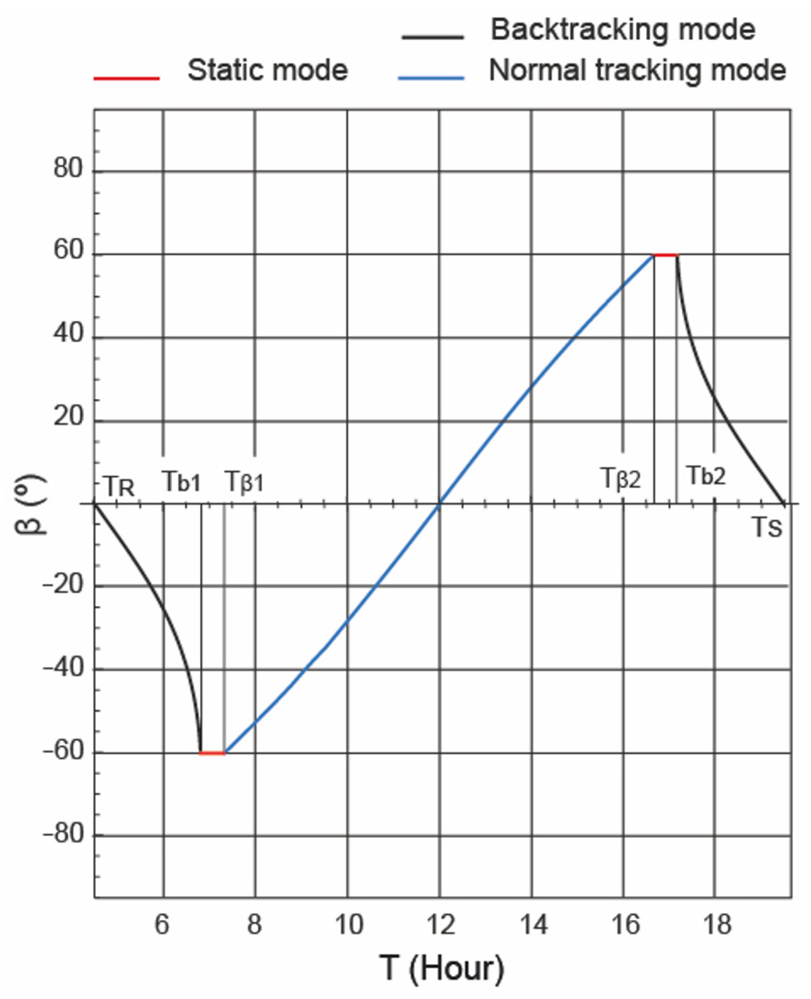
2.1.2. Horizontal Single-Axis Tracker

A horizontal single-axis tracker has its axis of rotation aligned with the north–south axis. Therefore, the $PV$ field rotates from east to west, following the daily movement of the Sun. Furthermore, this east–west rotational movement has a limited tilt angle range (${\beta }_{max}$). This value is usually $\pm 60$(°) [19]. The structural system of a horizontal single-axis tracker is comprised of several elements: columns (1), beams (2), torsion tube (3), drive device ($DC$ motor and drivers) (4), and spherical bearings (5) (see Figure 3):

2.2. Differences Between PV Module Mounting Systems Under Study

The process of designing a $PV$ power plant begins with a feasibility study based, among other things, on the following points: (i) analysis of the energy resource, (ii) analysis of performance, (iii) analysis of reliability, (iv) analysis of initial cost. These points, which will influence the choice of $PV$ module mounting system, will be studied below:

(i)

Energy production. The availability of moving parts allows horizontal single-axis trackers to align the $PV$ field with the sun throughout the day. Therefore, these mounting systems improve energy production compared to fixed tilt angle systems [18]. However, this improvement in production depends on the location of the $PV$ power plant. Several questions arise with regard to the energy production of horizontal single-axis trackers: Do they obtain energy gain at all times of the year? Do they obtain energy gain throughout the day? These questions will be analysed in this experimental and theoretical study.

(ii)

Reliability. Moving parts in a horizontal single-axis tracker complicate the reliability of the system, as they increase the risk of mechanical failure. As fixed tilt angle systems lack moving parts, these systems are very reliable. In contrast, horizontal single-axis trackers are less reliable, as their operating principle is based on the movement of the $PV$ field. Martin et al. [20] evaluated two $PV$ power plants equipped with fixed tilt angle systems and one $PV$ power plant equipped with horizontal single-axis trackers. The study covered several years of operation, concluding that fixed tilt angle systems were more reliable than horizontal single-axis trackers.

(iii)

Durability. Fixed tilt angle systems have no mechanical problems, due to the simplicity of their components. In contrast, horizontal single-axis trackers, with moving parts, require more maintenance and have a shorter lifespan.

(iv)

Simplicity of installation. Moving parts in a horizontal single-axis tracker complicate installation work. Therefore, fixed tilt angle systems are easier to install than horizontal single-axis trackers.

(v)

Maintenance costs. Moving parts in a horizontal single-axis tracker increase maintenance. Therefore, fixed tilt angle systems have lower maintenance costs than horizontal single-axis trackers. There is no standardised method for determining maintenance costs [36]. However, many authors use the report by the National Renewable Energy Laboratory [37] to calculate them; the criteria followed in this report, to calculate the annual maintenance cost, are as follows: (i) $0.5\%$ of the initial cost for fixed tilt angle systems, and (ii) $1\%$ of the initial cost for horizontal single-axis trackers. Other authors consider that the maintenance costs of horizontal single-axis trackers are double those considered for fixed tilt angle systems [37]. If the maintenance required is minimal, as in the case of fixed tilt angle systems, $PV$ plants installed in remote locations benefit greatly, as the number of regular checks is reduced.

(vi)

Initial costs. The absence of moving parts also influences initial costs, as it facilitates the installation of the mounting system. Fixed tilt angle systems have lower initial costs than horizontal single-axis trackers. Horizontal single-axis trackers are $50\%$ more expensive than fixed tilt angle systems [38]. This feature is a determining factor in smaller-scale $PV$ installations or projects with limited budgets.

(vii)

Vulnerability to extreme environmental factors. According to a report by the United Nations Intergovernmental Panel on Climate Change ($IPCC$), climate change will notably increase wind loads and extreme phenomena [39]. The operational characteristics of the $PV$ module mounting system make it susceptible to extreme environmental factors (strong winds or heavy snowfall) causing significant damage to $PV$ power plants [19]. Therefore, horizontal single-axis trackers are more susceptible to this type of damage.

(viii)

Limitation of geographical location. It has been demonstrated that the efficiency of fixed tilt angle systems decreases considerably in locations far from the equator [18], as their capacity to capture solar resources is not adequate throughout the year. In contrast, horizontal single-axis trackers are better suited to different latitudes [18], expanding the range of suitable geographical locations.

(ix)

Land occupation. A report by Mordon Intelligence [38] indicates that the density of $PV$ modules per square metre using horizontal single-axis trackers is between $25\%$ and $35\%$ higher than the use of fixed tilt angle systems.

(x)

Budgetary considerations. When making a decision about the choice of $PV$ module mounting system, the initial investment must be weighed against the expected return on investment. Although horizontal single-axis trackers offer higher performance, they also offer higher initial costs. In contrast, fixed tilt angle systems offer the opposite. Therefore, it may happen that the higher initial cost of a project makes it unviable.

(xi)

Environmental impact. From the point of view of environmental impact, horizontal single-axis trackers offer greater environmental benefits, as they generate more energy [18].

3. Methodology

The proposed methodology consists of four main steps: (i) choice of solar irradiance estimation model, (ii) theoretical study, (iii) study under real operating conditions, and (iv) comparison of these studies. Figure 4 shows a flowchart summarising the proposed methodology. Please note that in steps (ii) and (iii) there are several possible studies related to the horizontal single-axis tracker. In a fixed tilt angle system, the $PV$ field always occupies the same position from sunrise to sunset. In contrast, in a horizontal single-axis tracker under real operating conditions there are three modes of operation (backtracking mode, static mode, normal tracking mode). This mode of operation will be called Scenario 1; this is the real scenario, as it takes into account the movement limit ($\pm {\beta }_{max}$) of the $PV$ field and the backtracking mode. However, there are studies that consider that the solar tracker is in normal tracking mode from sunrise to sunset (Scenario 2), and that, therefore, the limit movement has an angle of $\pm 90$(°) (this case is unrealistic).

This section presents the experimental configuration and the evaluation indicators defined to analyse the energy performance of the two $PV$ module mounting systems under study.

3.1. Choice of Solar Irradiance Estimation Model

In the literature, there are many models for estimating the incident solar irradiance ($I_t$) on the $PV$ field of $PV$ module mounting systems. All the models consider that this solar irradiance can be decomposed into three components [40]: beam component ($I_{bt}$), diffuse component ($I_{dt}$), and reflected component ($I_{rt}$). All the models use the same equations to determine $I_{bt}$ and $I_{rt}$. Equations (1) and (3) are used to calculate these components. In contrast, there is no single equation for calculating the diffuse component. Each model has its own equation. These models can be classified as isotropic or anisotropic. The Liu–Jordan model [41], the Badescu model [42], and the Koronakis model [43] are isotropic models. And the Klucher model [44], the Pérez model [45], the Hay–Davies model [46], the $HDKR$ model [47], etc., are anisotropic models. In this study, we used an anisotropic model. Several studies have shown that anisotropic models obtain better results than isotropic models, but they are more complex to use [48]. The Klucher model is more complex and obtains good results in the anisotropic model segment [49]. Therefore, we will use the Klucher model, defined by Equation (4). The three components of the incident solar irradiance ($I_t$) on the $PV$ field are shown below:

Beam component

The researchers consider that the beam component is the geometric relationship between the horizontal surface and the surface of the photovoltaic field. The beam component can be calculated using the following equation [40]:

$$I_{bt}\left(n,T,\beta \right)=I_{bh}\left(n,T\right)·{\displaystyle \frac{cos{\theta }_i\left(n,T\right)}{cos{\theta }_z\left(n,T\right)}}$$

(1)

$$R_b={\displaystyle \frac{cos{\theta }_i\left(n,T\right)}{cos{\theta }_z\left(n,T\right)}}$$

(2)

where $I_{bh}\left(n,T\right)$ is the hourly distribution of the beam horizontal solar irradiance (W/m²), $R_b$ is the variable geometric factor, which is a ratio of tilted and horizontal solar beam irradiance, n is the ordinal of the day (day), T is the solar time (h), ${\theta }_z$ is the zenith angle of the sun (°), and ${\theta }_i$ is the incident angle (°).

Reflected component

The researchers assume that the reflected component depends on numerous factors, and, therefore, it is practically impossible to determine it precisely. The reflected component can be estimated using the following equation proposed by Liu and Jordan [41]:

$$I_{rt}\left(n,T,\beta \right)=(I_{bh}\left(n,T\right)+I_{dh}\left(n,T\right))·{\rho }_g·\left({\displaystyle \frac{1-cos\beta \left(n,T\right)}{2}}\right)$$

(3)

where $I_{bh}\left(n,T\right)$ is the hourly distribution of the beam horizontal solar irradiance (W/m²), $I_{dh}\left(n,T\right)$ is the hourly distribution of the diffuse horizontal solar irradiance (W/m²), n is the ordinal of the day (day), T is the solar time (h), $\beta$ is the tilt angle of the $PV$ field (°), and ${\rho }_g$ is the ground reflectance ($dimensionless$).

Diffuse component

This component can be estimated using the following equation proposed by Klucher [44]:

$$\begin{array}{c}{I}_{dt}\left(n,T,\beta \right)=I_{dh}\left(n,T\right)·\left({\displaystyle \frac{1+cos\beta \left(n,T\right)}{2}}\right)·\left(1+F_k·{sin}^3\left({\displaystyle \frac{\beta \left(n,T\right)}{2}}\right)\right)\hfill \\ \hfill ·\left(F_k·{cos}^2\left({\theta }_i\left(n,T\right)\right)·{cos}^3\left({\theta }_z\left(n,T\right)\right)\right)\end{array}$$

(4)

$$F_k=1-{\left({\displaystyle \frac{I_{dh}}{I_{gh}}}\right)}^2$$

(5)

where $I_{gh}\left(n,T\right)$ is the hourly distribution of the global horizontal solar irradiance (W/m²), $I_{dh}\left(n,T\right)$ is the hourly distribution of the diffuse horizontal solar irradiance (W/m²), n is the ordinal of the day (day), T is the solar time (h), $\beta$ is the tilt angle of the $PV$ field (°), and $F_k$ is the Klucher coefficient ($dimensionless$).

To operate with Equations (1)–(4), it is essential to know $I_{bh}$, $I_{dh}$, $\beta$, ${\theta }_z$, ${\theta }_i$, and ${\rho }_g$. These parameters can be determined as follows:

(i)

Determination of $\beta$.

The equations for calculating this parameter for the fixed tilt angle system and for the three operating modes of the horizontal single-axis tracker are as follows:

Fixed tilt angle system:

$$\beta =constant$$

(6)

Backtracking mode (horizontal single-axis tracker) [23]:

$${\beta }_B={\theta }_t-arccos\left({\displaystyle \frac{e_t}{W}}cos{\theta }_t\right)$$

(7)

where ${\theta }_t$ is the solar transversal angle (°), $e_t$ is the pitch (m), and W is the width of a mounting system (m).

Static mode (horizontal single-axis tracker) [23]:

$${\beta }_s=\pm {\beta }_{max}$$

(8)

At sunrise, ${\beta }_s=-{\beta }_{max}$, and at sunset, ${\beta }_s=+{\beta }_{max}$.

Normal tracking mode (horizontal single-axis tracker) [23]:

$$\beta ={\theta }_t=arctan(tan{\theta }_z\left|sin{\gamma }_s\right|)$$

(9)

where ${\theta }_t$ is the solar transversal angle (°), ${\theta }_z$ is the zenith angle of the sun (°), and ${\gamma }_s$ is the azimuth of the sun (°).

(ii)

Determination of the $cos{\theta }_z$.

The equation for calculating this parameter for both $PV$ module mounting systems is as follows [23]:

$$cos{\theta }_z=sin\delta sin\lambda +cos\delta cos\lambda cos\omega$$

(10)

where $\delta$ is the solar declination (°), $\lambda$ is the latitude (°), and $\omega$ is the hour angle (°).

(iii)

Determination of the $cos{\theta }_i$.

The equations for calculating this parameter for the fixed tilt angle system and for the three operating modes of the horizontal single-axis tracker are as follows:

Fixed tilt angle system [50]:

$$\begin{array}{c}cos{\theta }_i=sin\delta ·sin\lambda ·cos\beta -sin\delta ·cos\lambda ·sin\beta ·cos\gamma +cos\delta ·cos\lambda ·cos\beta ·cos\omega \hfill \\ \hfill +cos\delta ·sin\lambda ·sin\beta ·cos\gamma ·cos\omega +cos\delta ·sin\beta ·sin\gamma ·sin\omega \end{array}$$

(11)

where $\delta$ is the solar declination (°), $\lambda$ is the latitude (°), $\beta$ is the tilt angle (°), $\gamma$ is the azimuth angle (°), and $\omega$ is the hour angle (°). Duffie and Beckman propose two restrictions to apply Equation (11) [50]: (1) ${\theta }_i$ can exceed 90 (°), which means that the sun is behind the $PV$ field, and (2) the earth is not blocking the sun.

Backtracking mode (horizontal single-axis tracker) [23]:

$$cos{\theta }_i=cos{\beta }_{B}cos{\theta }_z+sin{\beta }_{B}sin{\theta }_{z}cos\left({\gamma }_s-\gamma \right)$$

(12)

Static mode (horizontal single-axis tracker) [23]:

$$cos{\theta }_i=cos{\beta }_{max}cos{\theta }_z+sin{\beta }_{max}sin{\theta }_{z}cos\left({\gamma }_s-\gamma \right)$$

(13)

Normal tracking mode (horizontal single-axis tracker) [23]:

$$cos{\theta }_i=\sqrt{{cos}^2{\theta }_z+{cos}^2\delta {sin}^2\omega }$$

(14)

where $\delta$ is the solar declination (°), $\beta$ is the tilt angle (°), ${\gamma }_s$ is the azimuth of the Sun (°), $\gamma$ is the azimuth angle (°), and $\omega$ is the hour angle (°).

(iv)

Determination of ${\rho }_g$.

The quotient between $I_{rh}\left(n,T\right)$ and $I_{gh}\left(n,T\right)$ is ${\rho }_g$, and it is strongly dependent on the type of soil surrounding the $PV$ field. A detailed study on the calculation of ${\rho }_g$ was presented by [51]. This study characterised several types of materials used in the building sector. For example: for weathered concrete, ${\rho }_g=0.22$; for red brick, dark paints, ${\rho }_g=0.27$; for light brick, light paints, ${\rho }_g=0.60$; for green vegetation, ${\rho }_g=0.20$. If the characteristics of the soil are unknown, $0.2$ is usually taken.

The parameters $I_{bh}$ and $I_{dh}$ are determined in the following sections.

Equations (15) and (17) can be used to determine the incident solar irradiation on the $PV$ field, for fixed tilt angle systems and for horizontal single-axis trackers, respectively:

Fixed tilt angle system [50]:

$$H_t\left(n\right)={\int }_{T_R\left(n\right)}^{T_S\left(n\right)}{I}_t(n,T,\beta )dT$$

(15)

where $T_R$ is the sunrise solar time (h), and where $T_S$ is the sunset solar time (h).

Horizontal single-axis tracker [23]:

$$H_t\left(n\right)={\int }_{T_R\left(n\right)}^{T_S\left(n\right)}{I}_t(n,T,\beta )dT$$

(16)

$$\begin{array}{c}{H}_t\left(n\right)={\int }_{T_R\left(n\right)}^{T_{b1}\left(n\right)}{I}_t\left(n,{\beta }_B,T\right)dT+{\int }_{T_{b1}\left(n\right)}^{T_{\beta 1}\left(n\right)}{I}_t\left(n,-{\beta }_{max},T\right)dT+\hfill \\ \hspace{1em}\hspace{1em}\hspace{1em}\hspace{1em}\hspace{1em}\hspace{1em}\hspace{1em}\hspace{1em}\hspace{1em}{\int }_{T_{\beta 1}\left(n\right)}^{T_{\beta 2}\left(n\right)}{I}_t\left(n,{\theta }_t,T\right)dT+{\int }_{T_{\beta 2}\left(n\right)}^{T_{b2}\left(n\right)}{I}_t\left(n,{\beta }_{max},T\right)dT+\\ \hfill {\int }_{T_{b2}\left(n\right)}^{T_S\left(n\right)}{I}_t\left(n,{\beta }_B,T\right)dT\end{array}$$

(17)

where $T_R$ is the sunrise solar time (h), $T_{b1}$ is the end of the backtracking mode (h), $T_{\beta 1}$ is the start of the normal tracking mode (h), $T_{\beta 2}$ is the end of the normal tracking mode (h), $T_{b2}$ is the start of the backtracking mode (h), and $T_S$ is the sunset solar time (h).

3.2. Theoretical Study

The solar irradiance on a horizontal surface, $I_{bh}$ and $I_{dh}$, necessary to calculate the different components of the incident solar irradiance on the $PV$ field can be determined from a theoretical point of view. These components are determined below:

(i)

Determination of $I_{bh}$. As this was a theoretical study, the Hottel model [52] was used to determine the $I_{bh}$. The Hottel model is a model of clear skies. Hottel proposes Equation (18) to determine the beam horizontal solar irradiance in clear atmospheres [52]:

$$I_{bh}\left(n,T\right)=I_0\left(n\right)·cos{\theta }_z\left(n,T\right)·{\tau }_b\left(n,T\right)$$

(18)

where $I_0$ is the extraterrestrial solar irradiance measured in the plane normal to the Sun’s rays (W/m²), and where ${\tau }_b$ is the atmospheric transmittance for beam solar irradiance ($dimensionless$); ${\tau }_b$ can be calculated using the following equation [52]:

$${\tau }_b=a_0+a_1·e^{-k/cos{\theta }_z}$$

(19)

where $a_0$, $a_1$, and k are empirical constants. If the standard atmosphere has 23 (km) of visibility, they can be calculated using the following equations:

$$\begin{array}{cc}\hfill a_0& =0.4237-0.00821{(6-A)}^2\hfill \end{array}$$

(20)

$$\begin{array}{cc}\hfill a_1& =0.5051-0.0059{(6.5-A)}^2\hfill \end{array}$$

(21)

$$\begin{array}{cc}\hfill k& =0.2711-0.01858{(2.5-A)}^2\hfill \end{array}$$

(22)

where A is the height above sea level of the location (km). For altitudes lower than $2.5$ (km), the empirical constants ($a_0$, $a_1$, k) have to be multiplied by their corresponding correction factors ($r_0$, $r_1$, $r_k$). These correction factors were tabulated for four different types of climate [52].

(ii)

Determination of $I_{dh}$. As this was a theoretical study, the Liu–Jordan model [53] was used to determine the $I_{dh}$. The Liu–Jordan model is a model of clear skies. Liu and Jordan proposed Equation (23), to determine the diffuse horizontal solar irradiance in clear atmospheres [53]:

$$I_{dh}\left(n,T\right)=I_0\left(n\right)·cos{\theta }_z\left(n,T\right)·{\tau }_d\left(n,T\right)$$

(23)

where $I_0$ is the extraterrestrial solar irradiance measured in the plane normal to the Sun’s rays (W/m²), and where ${\tau }_d$ is the atmospheric transmittance for diffuse solar irradiance ($dimensionless$); ${\tau }_d$ can be calculated using the following equation [53]:

$${\tau }_d=0.271-0.294·{\tau }_b$$

(24)

3.3. Study Under Real Operating Conditions

For this section, the solar irradiance on a horizontal surface was determined in real operating conditions of the $PV$ module mounting systems.

In order to evaluate the $PV$ module mounting systems under study from the point of view of the incident solar irradiance on the $PV$ field, an experimental setup was needed to recreate real operating conditions. The experimental setup consisted of an annual fixed tilt angle system and a horizontal single-axis tracker. The experimental setup is shown in Figure 5:

The characteristics of the experimental setup were as follows:

(i)

Location of the experimental setup. In order to be able to compare both $PV$ module mounting systems, it was necessary that the installation location was the same. The experimental setup was installed at the Department of Electrical Engineering of the University of Oviedo (Gijón, Spain) (latitude $43°{31}^{\prime }{22}^{\prime \prime }$ N, longitude $05°{43}^{\prime }{07}^{\prime \prime }$ W, elevation 28 (m) above sea level). Gijón is characterised by a temperate oceanic climate typical of Spain’s Atlantic coast, with cool summers and wet and mostly mild winters. The code assigned to Gijón under the Köppen climate classification is $C_{fb}$.

(ii)

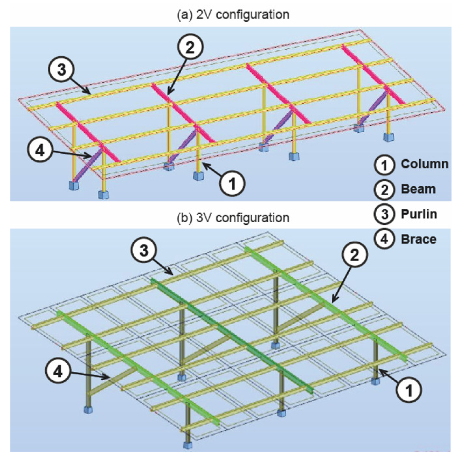
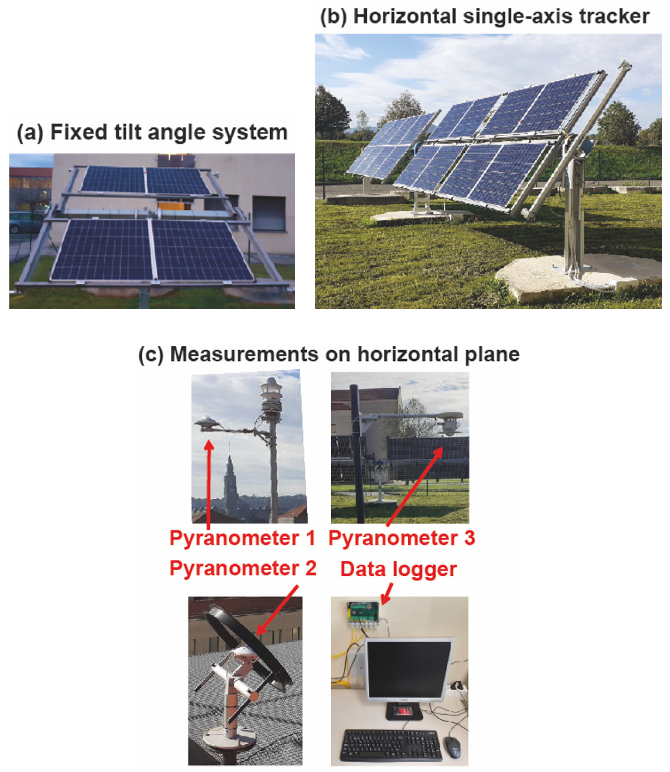
The ground-mounted $PV$ power plant. This type of $PV$ power plant is composed of fixed tilt angle systems (see Figure 5a). The following considerations were taken into account in the design of this $PV$ plant: (1) the configuration was $2Vx2$; (2) the fixed tilt angle system was south-facing; (3) the $PV$ field had a tilt angle of $33.5$(°); this angle is the optimum angle according to the Jacobson equation [18]; (4) the longitudinal spacing for maintenance was 4 (m); (5) the transversal installation distance was $0.30$ (m); (6) the transverse and longitudinal installation distance between the $PV$ modules was $0.025$ (m), due to the clamps; (7) the $PV$ module used was the CanadianSolar CS3U-355PB-FG, 355 (Wp).

(iii)

The single-axis tracking $PV$ power plant. This type of $PV$ power plant is composed of horizontal single-axis trackers (see Figure 5b). The following considerations were taken into account in the design of this $PV$ plant: (1) the configuration was $1Vx8$; (2) the pitch was $6.5$ (m); (3) the limit of movement was $\pm 60$(°); (4) the transversal installation distance was $0.30$ (m); (5) the transverse and longitudinal installation distance between the $PV$ modules was $0.025$ (m), due to the clamps; (6) the $PV$ module used was the CanadianSolar CS3U-355PB-FG, 355 (Wp).

(iv)

Measuring instruments (see Figure 5c). The measurement system consisted of three pyranometers. The experimental measurements taken were global horizontal solar irradiance (Pyranometer 1), diffuse horizontal solar irradiance (Pyranometer 2), and reflected solar irradiance (Pyranometer 3). Its characteristics were as follows: (a) the same type of pyranometer was used; (b) the pyranometer used was the $CMP11$ model manufactured by Kipp & Zonen; (c) the accuracy class was Class A (secondary standard); (d) the pyranometer’s measurement range was 0–4000 (W/m²); (e) the expected daily accuracy was less than $2\%$. Several sources of error can be associated with any experimental process, such as calibration, precision, methodology of experiments, etc. [54]. These sources of error affect the experimental results [54]. In this study, solar irradiances were measured directly; therefore, the uncertainty of the measurements was defined by the accuracy of the pyranometers [55]. As the uncertainty of the pyranometers was less than $3\%$, the experimental data can be considered to be highly accurate [55].

(v)

Duration of the test campaign. The test campaign was carried out in 2022. The pyranometers measured solar irradiance every second, calculating the average every minute. Data were recorded for one year. During the data collection campaign, no incidents occurred in the horizontal single-axis tracker. Therefore, in our study the reliability of the horizontal single-axis solar tracker was high. It is also true that the wind loads supported by the horizontal single-axis tracker were low. The initial cost of the horizontal single-axis tracker prototype was approximately $1.8$ times higher than the fixed tilt angle system prototype.

3.4. Assessment Indicators for the Comparison of Studies

In this study, the two $PV$ module mounting systems under study were compared, in terms of the concept of energy gain [18]. The energy gain ($EG$) could be calculated as the difference between the energy absorbed by the horizontal single-axis tracker and the energy absorbed by the fixed tilt angle system. The energy gains analysed were as follows: annual energy gain, monthly energy gain, and daily energy gain.

3.4.1. Annual Energy Gain

The annual energy gain ($AEG$) (%) parameter was used to make a comparison between the two $PV$ module mounting systems:

$$AEG={\displaystyle \frac{H_{tt}^a-H_{tf}^a}{H_{tf}^a}}·100$$

(25)

where $H_{tt}^a$ is the annual incident solar irradiation on the $PV$ field of the horizontal single-axis tracker (J/m²), and where $H_{tf}^a$ is the annual incident solar irradiation on the $PV$ field of the fixed tilt angle system (J/m²).

3.4.2. Monthly Energy Gain

The monthly energy gain ($MEG$) (%) parameter was used to make a comparison between the two $PV$ module mounting systems:

$$MEG={\displaystyle \frac{H_{tt}^m-H_{tf}^m}{H_{tf}^m}}·100$$

(26)

where $H_{tt}^m$ is the monthly incident solar irradiation on the $PV$ field of the horizontal single-axis tracker (J/m²), and where $H_{tf}^m$ is the monthly incident solar irradiation on the $PV$ field of the fixed tilt angle system (J/m²).

3.4.3. Daily Energy Gain

The daily energy gain ($DEG$) (%) parameter was used to make a comparison between the two $PV$ module mounting systems:

$$DEG={\displaystyle \frac{H_{tt}^d-H_{tf}^d}{H_{tf}^d}}·100$$

(27)

where $H_{tt}^d$ is the daily incident solar irradiation on the $PV$ field of the horizontal single-axis tracker (J/m²), and where $H_{tf}^d$ is the daily incident solar irradiation on the $PV$ field of the fixed tilt angle system (J/m²).

4. Results and Discussion

For this section, the incident solar irradiance on the $PV$ field under real operating conditions was analysed. The $PV$ module mounting systems under study were fixed tilt angle systems and horizontal single axis trackers. A theoretical analysis was also performed, to analyse the study in locations where no data were available under real operating conditions. Determining the hourly distribution of incident solar irradiance in both mounting systems was key to this study. To this end, several specific codes were developed with $Mathematica$ 11 software (see Figure A1). The assessment indicators used to study the incident solar irradiance on $PV$ power plants under real operating conditions were as follows: annual energy gain, monthly energy gain, and daily energy gain.

$PV$ power plants are comprised of a large number of $PV$ module mounting systems; therefore, shading between them is a fundamental parameter. A $PV$ power plant may comprise (i) fixed tilt angle systems, which are characterised by keeping the position of their $PV$ field constant from sunrise to sunset, and (ii) horizontal single-axis trackers, which have three operating modes (backtracking mode, static mode (${\beta }_{max}=\pm 60$(°)), and normal tracking mode). This operating mode is referred to as Scenario 1. If it is considered that there is only one $PV$ module mounting system, shading between them no longer exists; therefore, the solar tracker can be in normal tracking mode from sunrise to sunset (Scenario 2), so the limit movement has an angle of $\pm 90$(°).

4.1. $PV$ Module Mounting Systems Under Study

Three mounting systems were selected for the analysis of $PV$ power plants under real operating conditions.

Table 1. Specifications of the PV module mounting systems.

Specifications	PV Module Mounting System
	Fixed Tilt Angle System	Scenario 1	Scenario 2
Location	Gijon, (Spain)	Gijon, (Spain)	Gijon, (Spain)
Latitude	$43°{31}^{\prime }{22}^{\prime \prime }$ N	$43°{31}^{\prime }{22}^{\prime \prime }$ N	$43°{31}^{\prime }{22}^{\prime \prime }$ N
Longitude	$05°{43}^{\prime }{07}^{\prime \prime }$ W	$05°{43}^{\prime }{07}^{\prime \prime }$ W	$05°{43}^{\prime }{07}^{\prime \prime }$ W
Altitude (m)	28.0	28.0	28.0
Fixed tilt angle (°)	$33.5$	-	-
Tracking type	-	Horiz. single-axis tracker	Horiz. single-axis tracker
Type of control	-	Astronomical algorithm	Astronomical algorithm
Backtracking mode	-	Yes	No
Rotation angle (${\beta }_{max}$) (°)	-	$\pm 60$	$\pm 90$
Configuration	2Vx2	1Vx8	1Vx8
Pitch ($e_t$) (m)	6.5	6.5	6.5
Reflectance (${\rho }_g$)	0.3	0.3	0.3

shows their main technical and geographical characteristics. The criteria on which this choice of editing systems were based are as follows: (i) The fixed tilt angle system and horizontal single-axis tracker (Scenario 1) are the most commonly used mounting systems in $PV$ power plants [19], and (ii) the horizontal single-axis tracker (Scenario 2) is used in many studies that do not consider shading between $PV$ fields, and, although it is not a real case, it is interesting to analyse the differences with Scenario 1.

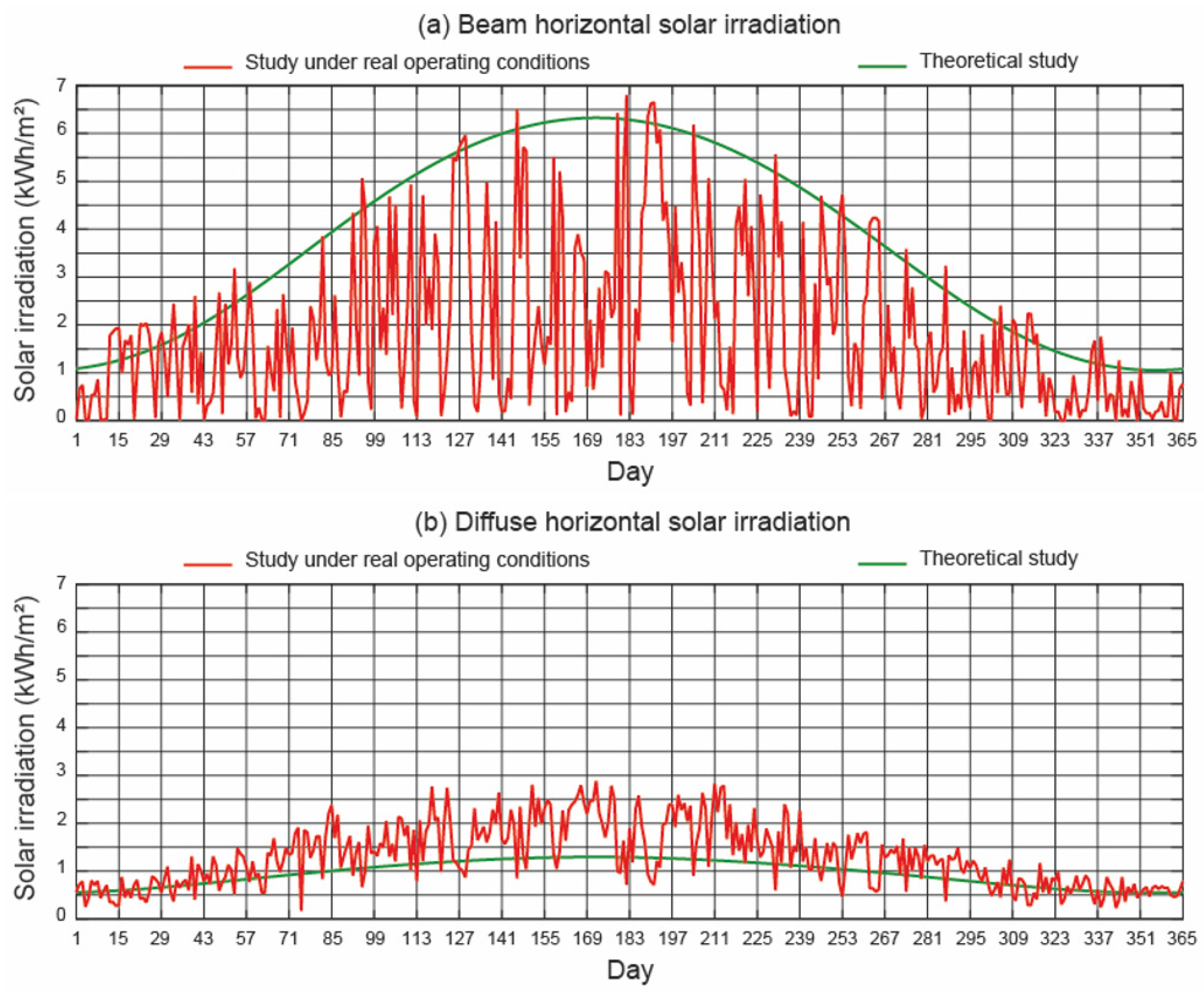
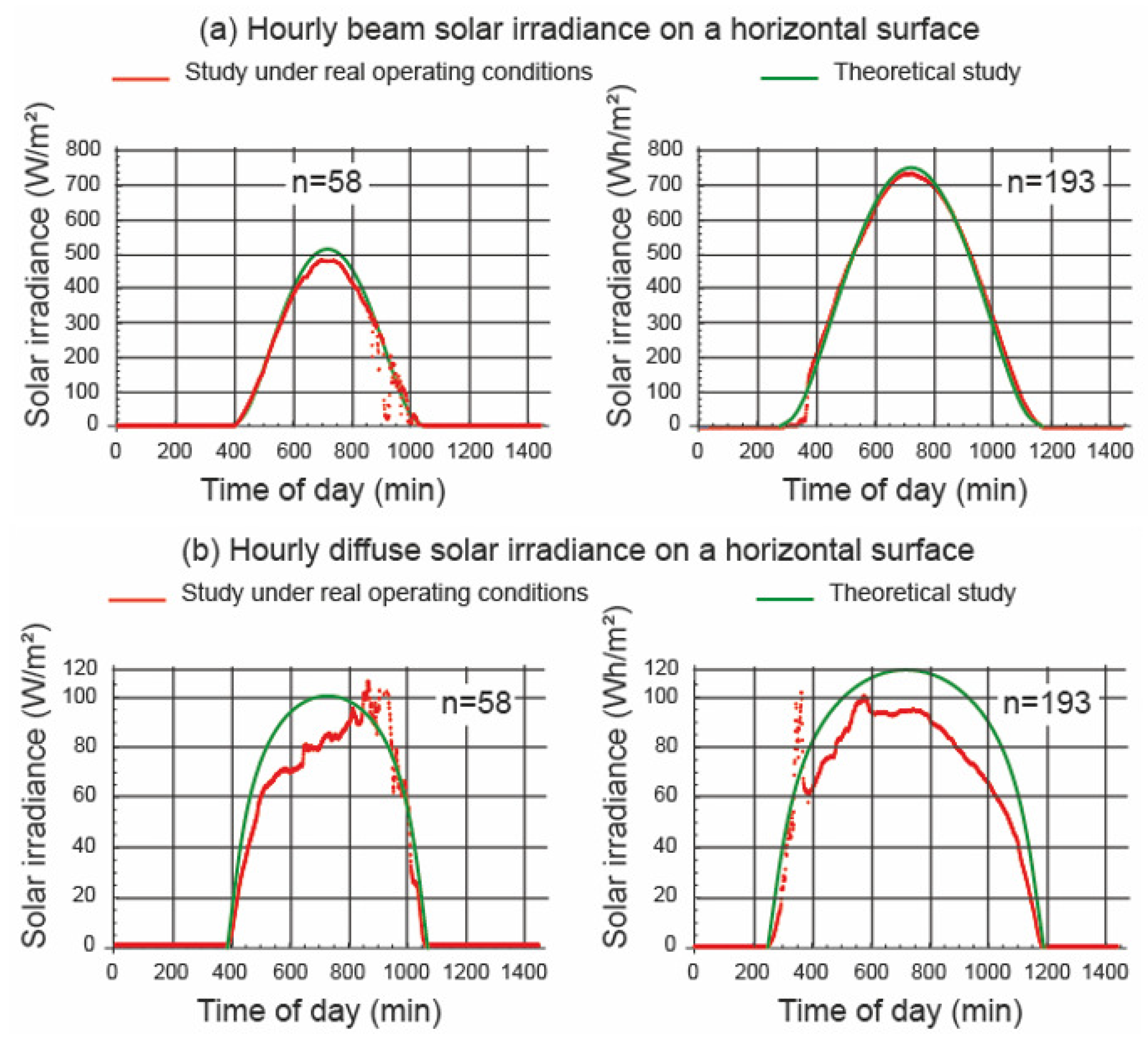
4.2. Solar Irradiation Data

The meteorological conditions of the location under study are a key factor in the comparison of $PV$ module mounting systems. Therefore, the solar irradiance data measured by pyranometers 1, 2, and 3 were used in the study under real operating conditions. On the other hand, the Hottel and Liu–Jordan models were used in the theoretical study.

Table 2. Monthly beam and diffuse horizontal solar irradiation in real operating conditions and in theoretical conditions.

Specifications	Theoretical Study		Real Operating Conditions
(kWh/m2)	Hbh	Hdh	Hbh	Hdh
January	40.61	18.72	32.49	18.71
February	60.46	21.25	39.80	25.48
March	107.37	29.29	34.68	43.57
April	145.29	33.44	76.77	48.20
May	181.50	38.35	85.39	53.73
June	188.72	38.76	71.84	63.20
July	188.63	39.16	110.49	56.94
August	163.34	35.95	65.80	51.70
September	120.78	30.26	68.96	38.03
October	82.16	25.66	35.47	33.40
November	46.99	19.57	25.63	20.61
December	33.95	17.24	15.82	17.67

shows the monthly beam and diffuse horizontal solar irradiation in real operating conditions and in theoretical conditions.

Figure 6 shows daily beam and diffuse solar irradiation on a horizontal surface under real operating conditions and under theoretical conditions:

Figure 7 shows hourly beam and diffuse solar irradiation on a horizontal surface under real operating conditions and under theoretical conditions:

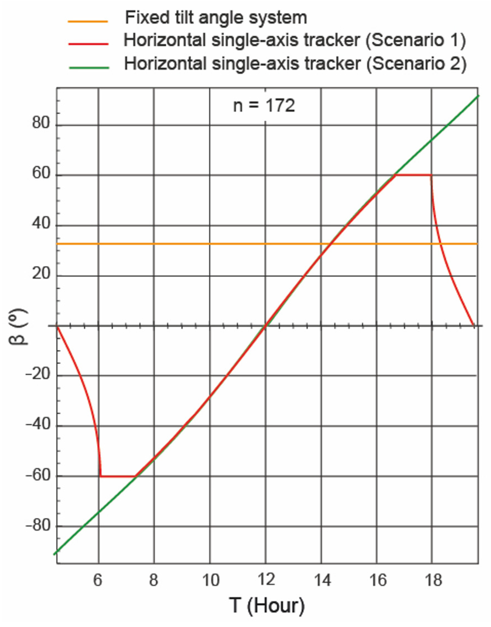
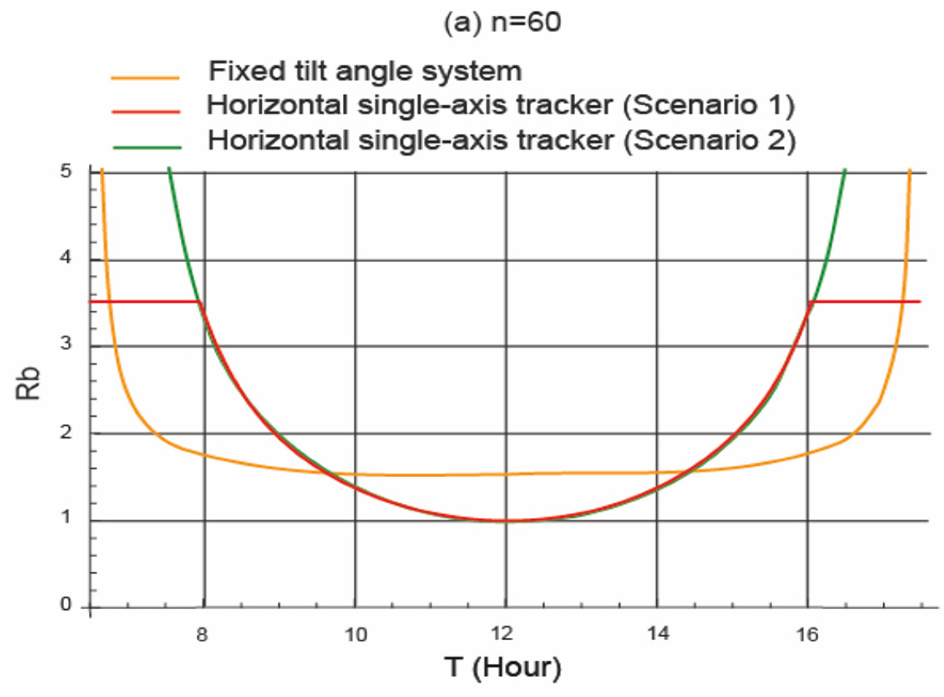
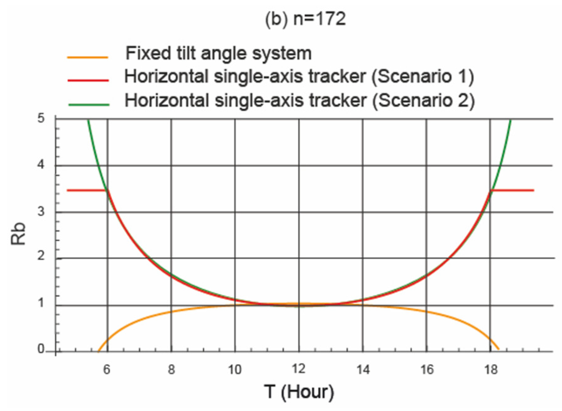
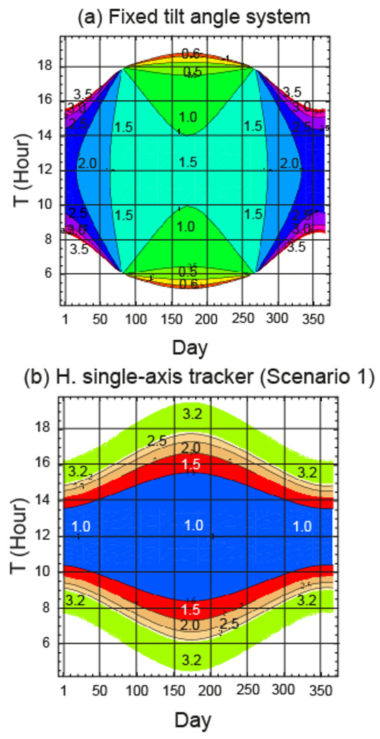
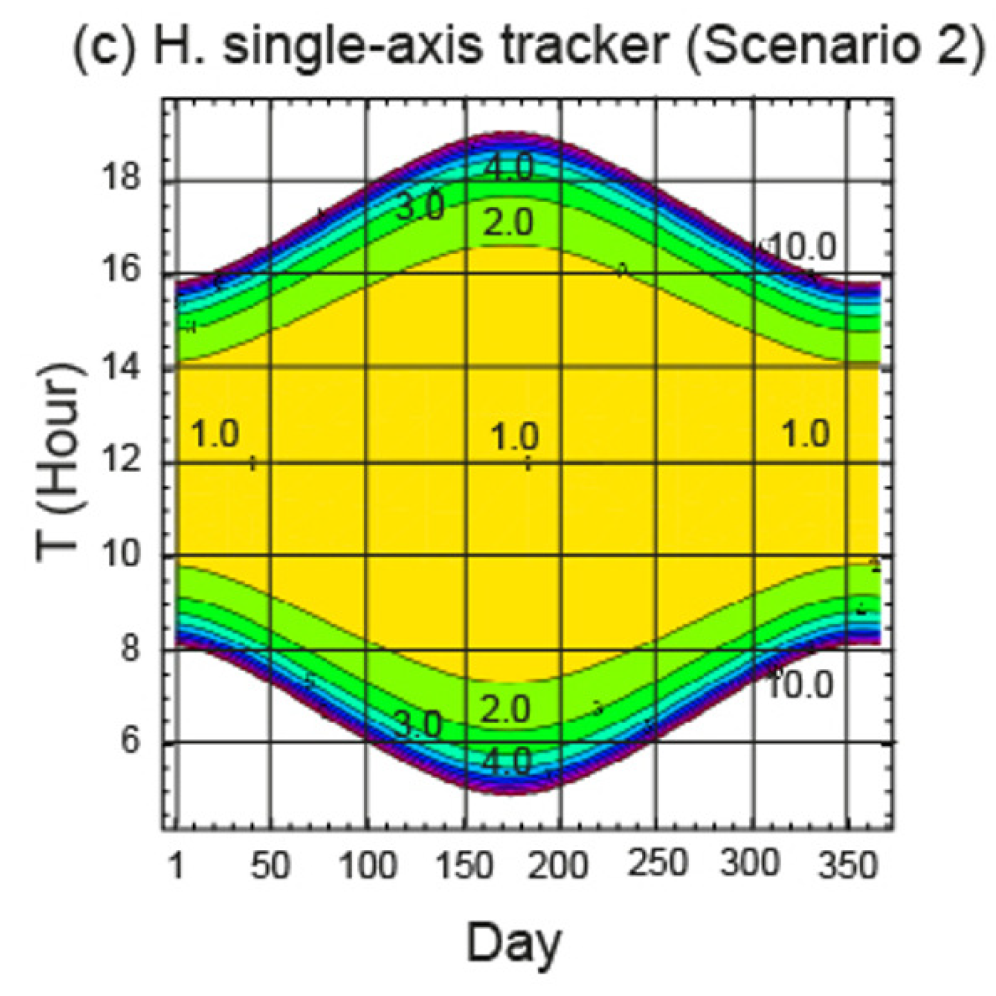
4.3. Analysis of the Angles of Incident Solar Irradiance on the PV Field

The parameter $\beta$ is present in the components of the solar irradiance incident on the $PV$ field in the two $PV$ module mounting systems under study. The equations in which it is present are (1), (3), and (4). Figure 8 shows the position of $\beta$ on 21 June ($n=172$) in the fixed tilt angle system, the horizontal single-axis tracker (Scenario 1), and the horizontal single-axis tracker (Scenario 2). In this figure, the variation of $\beta$ can be seen in (i) the fixed tilt angle system that remains constant from sunrise to sunset, (ii) the three operating modes (backtracking mode, static mode, normal tracking mode) of Scenario 1 of a horizontal single-axis tracker, and (iii) the only operating mode (normal tracking mode) of Scenario 2 of a horizontal single-axis tracker:

The parameter $R_b$ is present in the beam component of the incident solar irradiance on the PV field in the two PV module mounting systems under study. This dependency can be seen in Equation (1). Figure 9 shows the parameter $R_b$ on the 60th (1st March) and 172nd (21st June) ordinal days. The position of $\beta$ shown in Figure 8 gives rise to the parameter $R_b$ being as shown in Figure 9b.

According to Figure 9a, on day $n=60$ (1st March) the behaviour of $R_b$ of the fixed tilt angle system is significantly better in the middle of the day. In contrast, on day $n=172$ (21st June) the behaviour of $R_b$ of the horizontal single-axis tracker is significantly better in the middle of the day. As the incident solar irradiance on the $PV$ field is greater in the middle hours of the day, it can be deduced that the $R_b$ parameter behaves better in a particular mounting system during certain months of the year. Figure 10 shows these time periods.

If we compare scenarios 1 and 2 of a horizontal single-axis tracker, we can see that the $R_b$ parameter is higher in Scenario 2. However, we must bear in mind that Scenario 2 is not the one implemented in a $PV$ power plant.

Figure 10 shows the representation of the $R_b$ parameter throughout the year. In this figure, it can be seen that from days 70 to 277 the horizontal single-axis tracker has a higher $R_b$. Therefore, the beam component is greater in this mounting system.

4.4. Annual Energy Gain

For this section, the annual energy gain was analysed. Equation (25) was used for this purpose. The annual energy gain for the $PV$ module mounting systems under study is shown in Figure 11:

The following observations can be deduced from Figure 11:

(i)

In Scenario 1, an $AEG$ of approximately $13\%$ was obtained in the theoretical study. This result is in accordance with the results obtained by [56]. In the study under real operating conditions, this parameter decreased to approximately $8.5\%$.

(ii)

In Scenario 2, an $AEG$ of approximately $18\%$ was obtained in the theoretical study. This result is consistent with the results obtained by [18]. In the study under real operating conditions, this parameter decreased to approximately $10.5\%$.

(iii)

The best results were obtained in Scenario 2, both in the theoretical study and in the study under real operating conditions. However, Scenario 1 is the one implemented in a $PV$ power plant. The biggest difference was obtained in the theoretical study, of approximately $5.5\%$. In contrast, in the study under real operating conditions, this difference was approximately $2.2\%$.

4.5. Monthly Energy Gain

Although the annual analysis shows the overall behaviour of the mounting systems, a monthly analysis was necessary to determine the most appropriate mounting system for each period of time. Therefore, for this section the monthly energy gain ($MEG$) was analysed. Equation (26) was used for this purpose. The monthly energy gain for the $PV$ module mounting systems under study is shown in Figure 12:

The following observations can be deduced from Figure 12:

(i)

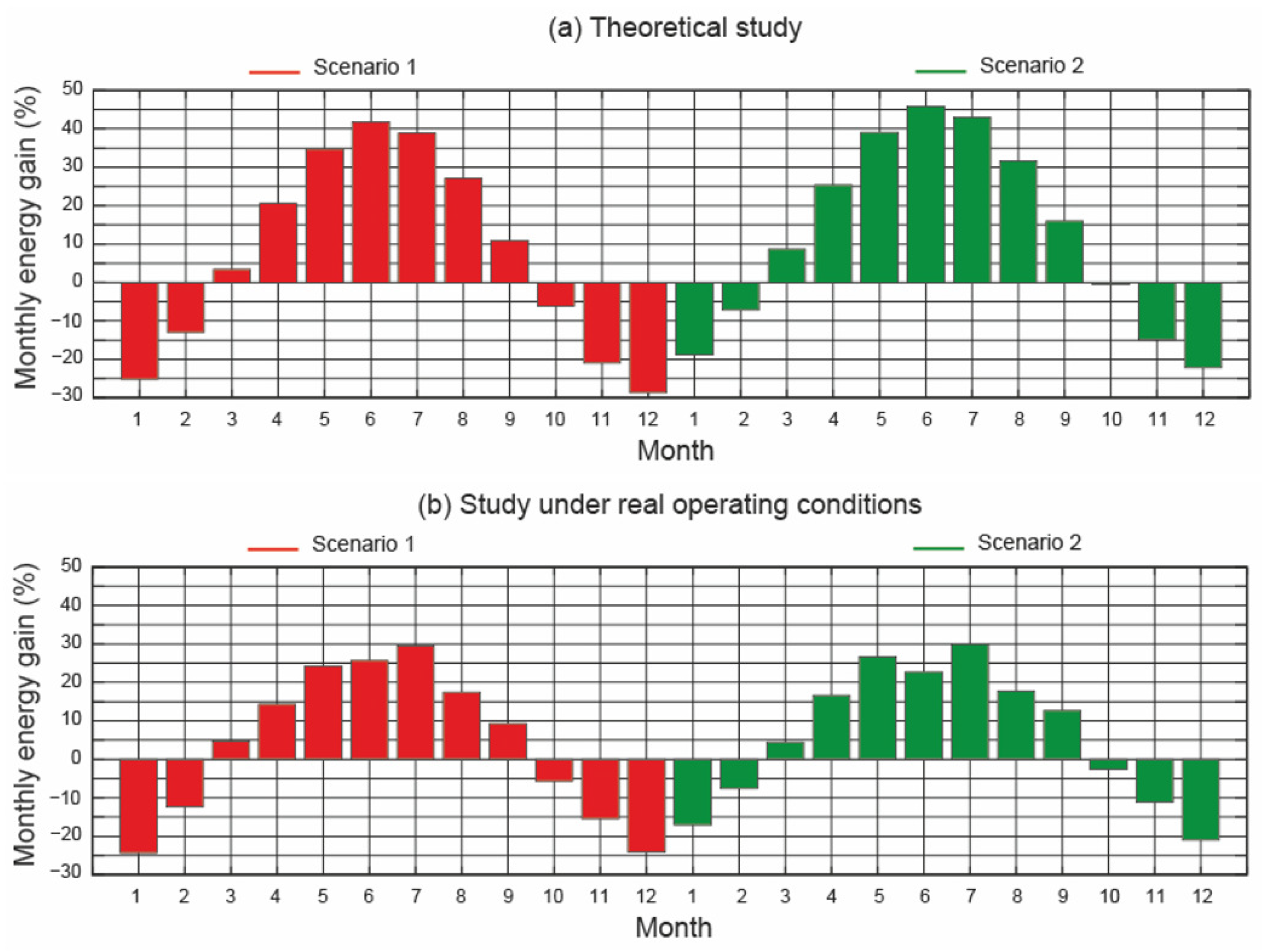
In the months of October, November, December, January, and February, the fixed tilt angle system performed better than the horizontal single-axis tracker, both in the theoretical study and in the study under real operating conditions. In the other months, the horizontal single-axis tracker performed better. Therefore, during the months of greatest incident solar irradiance, the horizontal single-axis tracker performed better. Figure 10, which shows the variation of $R_b$, explains this trend.

(ii)

In the theoretical study, the highest value of $MEG$ was in June and the worst was in December. These results were true in both the scenarios under study. In Scenario 1, these results were approximately $43\%$ and $-29\%$, respectively, and in Scenario 2 they were approximately $47\%$ and $-22\%$, respectively.

(iii)

In the study under real operating conditions, the best month was July and the worst month was December. This was true in both the scenarios under study. In Scenario 1, these results were approximately $30\%$ and $-24\%$, respectively, and in Scenario 2, approximately $30\%$ and $-21\%$, respectively.

4.6. Daily Energy Gain

For this section, the daily energy gain ($DEG$) was analysed. Equation (27) was used for this purpose. The daily energy gain for the $PV$ module mounting systems under study is shown in Figure 13.

The following observations can be deduced from Figure 13:

(i)

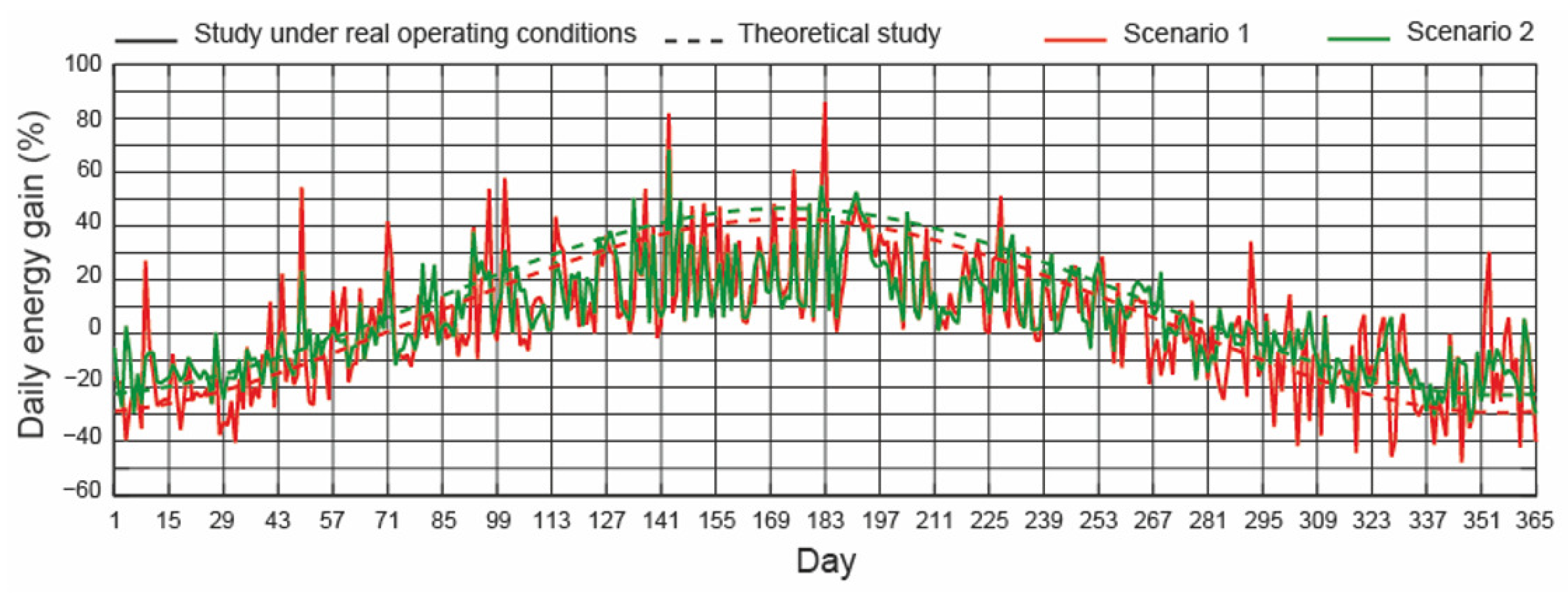
In Scenario 1, and considering the theoretical study, on days 1 to 69 and 278 to 365 the fixed tilt angle system performed better than the horizontal single-axis tracker. On the other days, the opposite happened. When Scenario 2 was considered, there was variation on these days: that is to say, on days 1 to 59 and 288 to 365 the fixed tilt angle system performed better than the horizontal single-axis tracker.

(ii)

Considering the theoretical study, in Scenario 1 the highest and lowest $DEG$ values were $43\%$ and $-30\%$, respectively, and in Scenario 2 these values were $47\%$ and $-23\%$, respectively.

(iii)

Considering the study under real operating conditions, in Scenario 1 the highest and lowest $DEG$ values were $58\%$ and $-47\%$, respectively, and in Scenario 2 these values were $68\%$ and $-30\%$, respectively.

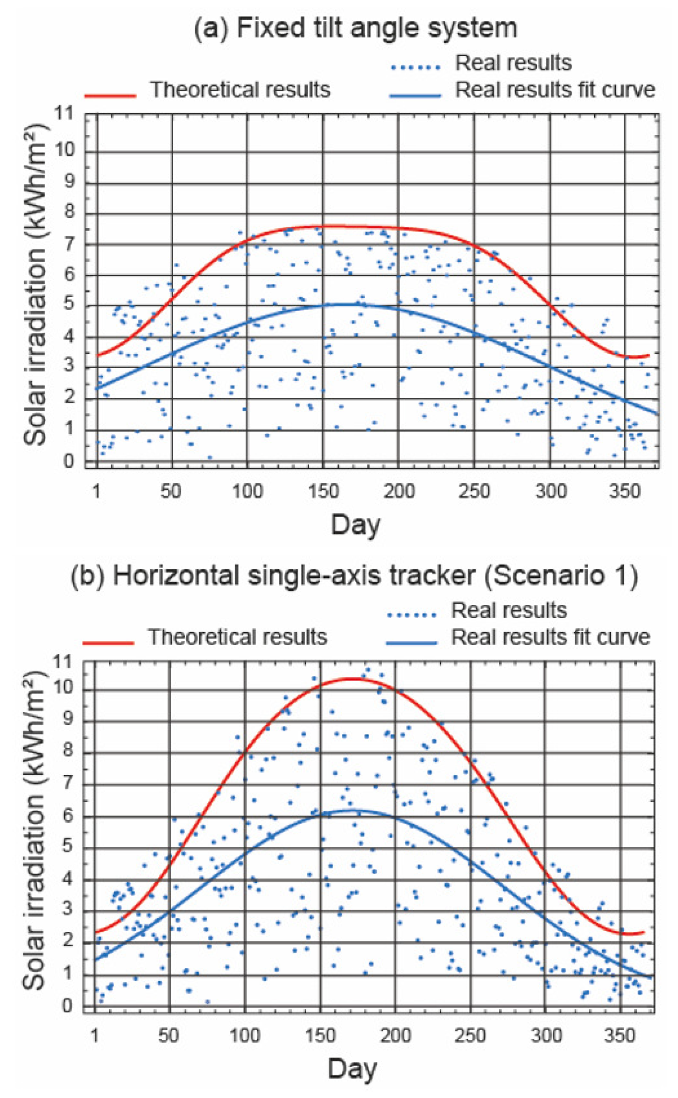
4.7. Regression Analysis Based on the Results of the Experiment

To compare the real and theoretical results of the daily incident solar irradiation of the different mounting systems, the real data were adjusted, using a fitting equation. Figure 14 shows the scatter diagram of the daily incident solar irradiation on the $PV$ field in the three mounting systems under study, together with the curve resulting from the fitting of the data using an exponential function of the following form:

$$y=a·e^{\left[-{\left({\displaystyle \frac{\left(x-c\right)}{b}}\right)}^2\right]}$$

(28)

where a, b, and c are parameters. The correlation coefficient ($R^2$) was also calculated for the fit equations. The results obtained were $0.842$ for the fixed tilt angle system, $0.825$ for the horizontal single-axis tracker (Scenario 1), and $0.822$ for the horizontal single-axis tracker (Scenario 2):

The following observations can be deduced from Figure 14:

(i)

Except in the fixed tilt angle system, the adjustment equations of the other two mounting systems provided very similar results.

(ii)

The theoretical study obtained better results than the study under real operating conditions in all three mounting systems.

5. Conclusions

This paper presents two energy studies: a study under real operating conditions and a theoretical study, of various photovoltaic module mounting systems (fixed tilt angle system, horizontal single-axis tracker). Fixed tilt angle systems are characterised by keeping the position of their photovoltaic field constant, from sunrise to sunset. The horizontal single-axis trackers that comprise photovoltaic power plants have three operating modes (Scenario 1) (backtracking mode, static mode (${\beta }_{max}=\pm 60$(°)), normal tracking mode). If we consider a horizontal single-axis tracker, it is not necessary to consider the shadows between mounting systems. Therefore, the horizontal single-axis tracker can be in normal tracking mode from sunrise to sunset (Scenario 2). In this case, the limit movement has an angle of $\pm 90$(°). The fixed tilt angle system was used as a baseline for comparison. The experimental setup was installed at the Department of Electrical Engineering of the University of Oviedo (Gijón, Spain) (latitude $43°{31}^{\prime }{22}^{\prime \prime }$ N, longitude $05°{43}^{\prime }{07}^{\prime \prime }$ W, elevation 28 (m) above sea level). Gijón is characterised by a temperate oceanic climate typical of Spain’s Atlantic coast, with cool summers and wet and mostly mild winters. The code assigned to Gijón under the Köppen climate classification is $C_{fb}$. Three assessment indicators were analysed (annual energy gain ($AEG$), monthly energy gain ($MEG$), daily energy gain ($DEG$)). In order to carry out the proposed studies, it was necessary to implement several specific codes to determine the components of the incident solar irradiance on the photovoltaic field of the mounting systems under study. The software used to implement the codes was $Mathematica$. The main conclusions obtained are summarised below:

(i)

The $AEG$ obtained was approximately $13\%$ and $8.5\%$ in the theoretical study and in the real study, respectively, in Scenario 1, and approximately $18\%$ and $10.5\%$, respectively, in Scenario 2. Scenario 2 obtained higher results than Scenario 1 in all the assessment indicators. But it must be considered that Scenario 1 is the real mode of operation.

(ii)

Considering the theoretical study and Scenario 1, the highest value of $MEG$ was in June ($43\%$) and the lowest was in December ($-29\%$). When the study was considered under real operating conditions, the highest result was in July ($30\%$) and the lowest was in December ($-24\%$).

(iii)

In scenario 1, on days 70 to 277 the horizontal single-axis tracker performed better. On the other days, the opposite occurred. Taking into account the theoretical study, the highest and lowest $DEG$ values were $43\%$ and $-30\%$, respectively. When the study was considered under real operating conditions, the highest and lowest $DEG$ values were $58\%$ and $-47\%$, respectively.

One possible line of future work is the analysis and implementation of a PV module mounting system with several fixed positions.

References

- IEA. Electricity 2024. Available online: https://iea.blob.core.windows.net/assets/18f3ed24-4b26-4c83-a3d2-8a1be51c8cc8/Electricity2024-Analysisandforecastto2026.pdf (accessed on 20 February 2025).
- IEA. Global Energy and Climate Model 2024. Available online: https://www.iea.org/reports/global-energy-and-climate-model (accessed on 20 February 2025).
- European Union. European Green Deal. 2019. Available online: https://commission.europa.eu/strategy-and-policy/priorities-2019-2024/european-green-deal/delivering-european-green-deal_en (accessed on 20 February 2025).
- European Union. Directive 2018/2001/EC, on the Promotion of the Use of Energy from Renewable Sources; European Union: Brussels, Belgium, 2018. [Google Scholar]
- Statista. Available online: https://www.statista.com/statistics/482733/energy-consumption-worldwide-sector (accessed on 20 February 2025).
- IEA. World Energy Outlook 2023. Available online: https://www.iea.org/reports/world-energy-outlook-2023?language=es (accessed on 20 February 2025).
- Aslam Bhatti, U.; Aslam Bhatti, M.; Tang, H.; Syam, M.S.; Mahrous Awwad, E.; Sharaf, M.; Yasin Ghadi, Y. Global production patterns: Understanding the relationship between greenhouse gas emissions, agriculture greening and climate variability. Environ. Res. 2024, 245, 118049. [Google Scholar] [CrossRef] [PubMed]
- Chen, H.; Wu, W.; Li, C.; Lu, G.; Ye, D.; Ma, C.; Ren, L.; Li, G. Ecological and environmental effects of global photovoltaic power plants: A meta-analysis. J. Environ. Manag. 2025, 373, 123785. [Google Scholar] [CrossRef] [PubMed]
- Ameur, A.; Berrada, A.; Loudiyi, K.; Aggour, M. Analysis of renewable energy integration into the transmission network. Electr. J. 2019, 32, 106676. [Google Scholar] [CrossRef]
- Weber, P.; Woerman, M. Intermittency or Uncertainty? Impacts of Renewable Energy in Electricity Markets. J. Assoc. Environ. Resour. Econ. 2024, 11, 1351–1385. [Google Scholar] [CrossRef]
- Vindel, J.M.; Trincado, E. Discontinuity in the production rate due to the solar resource intermittency. J. Clean. Prod. 2021, 321, 128976. [Google Scholar] [CrossRef]
- Zhu, H.; Hou, R.; Jiang, T.; Lv, Q. Research on energy storage capacity configuration for PV power plants using uncertainty analysis and its applications. Glob. Energy Interconnect. 2021, 4, 608–618. [Google Scholar] [CrossRef]
- Laugs, G.A.H.; Benders, R.M.J.; Moll, H.C. Balancing responsibilities: Effects of growth of variable renewable energy, storage, and undue grid interaction. Energy Policy 2020, 139, 111203. [Google Scholar] [CrossRef]
- Ahmed, R.; Sreeram, V.; Mishra, Y.; Arif, M.D. A review and evaluation of the state-of-the-art in PV solar power forecasting: Techniques and optimization. Renew. Sustain. Energy Rev. 2020, 124, 109792. [Google Scholar] [CrossRef]
- Qiao, J.; Meng, X.; Zheng, W.; Huang, P.; Xu, T.; Xu, Y. Optimization configuration method of energy storage considering photovoltaic power consumption and source-load uncertainty. IEEE Access 2025, 13, 9401–9412. [Google Scholar] [CrossRef]
- Bin Wali, S.; Hannan, M.A.; Reza, M.S.; Jern Ker, P.; Begum, R.A.; Abd Rahman, M.S.; Mansor, M. Battery storage systems integrated renewable energy sources: A biblio metric analysis towards future directions. J. Energy Storage 2021, 35, 102296. [Google Scholar] [CrossRef]
- Marocco, P.; Ferrero, D.; Gandiglio, M.; Ortiz, M.M.; Sundseth, K.; Lanzini, A.; Santarelli, M. A study of the techno-economic feasibility of H2-based energy storage systems in remote areas. Energy Convers. Manag. 2020, 211, 112768. [Google Scholar] [CrossRef]
- Barbón, A.; Fortuny Ayuso, P.; Bayón, L.; Silva, C.A. A comparative study between racking systems for photovoltaic power systems. Renew. Energy 2021, 180, 424–437. [Google Scholar] [CrossRef]
- Gonvarri Solar Steel. Available online: https://www.gsolarsteel.com/ (accessed on 20 February 2025).
- Martín-Martínez, S.; Cañas-Carretón, M.; Honrubia-Escribano, A.; Gómez-Lázaro, E. Performance evaluation of large solar photovoltaic power plants in Spain. Energy Convers. Manag. 2019, 183, 515–528. [Google Scholar] [CrossRef]
- Future Market Insights, Solar Trackers Market: Solar Trackers Market Analysis by Single-Axis and Dual-Axis for 2023 to 2033. Available online: https://www.futuremarketinsights.com/reports/solar-trackers-market#:~:text=The%20global%20solar%20trackers%20market,to%20\protect\@normalcr\relaxrenewable%20energy%20sources%20grows (accessed on 20 February 2025).
- Mordor Intelligence. Available online: https://www.mordorintelligence.com/industry-reports/solar-tracker-market (accessed on 20 February 2025).
- Barbón, A.; Carreira-Fontao, V.; Bayón, L.; Silva, C.A. Optimal design and cost analysis of single-axis tracking photovoltaic power plants. Renew. Energy 2023, 211, 626–646. [Google Scholar] [CrossRef]
- Barbón, A.; Martínez-Suárez, J.; Bayón, L.; Bayón-Cueli, C. Photovoltaic power plants with horizontal single-axis trackers: Influence of the movement limit on incident solar irradiance. Appl. Sci. 2025, 15, 1175. [Google Scholar] [CrossRef]
- Sun, L.; Bai, J.; Kumar Pachauri, R.; Wang, S. A horizontal single-axis tracking bracket with an adjustable tilt angle and its adaptive real-time tracking system for bifacial PV modules. Renew. Energy 2024, 221, 119762. [Google Scholar] [CrossRef]
- Berrian, D.; Chhapia, G.; Linder, J. Performance of land productivity with single-axis trackers and shade-intolerant crops in agrivoltaic systems. Appl. Energy 2025, 384, 125471. [Google Scholar] [CrossRef]
- Ge, Z.; Xu, Z.; Li, J.; Xu, J.; Xie, J.; Yang, F. Technical-economic evaluation of various photovoltaic tracking systems considering carbon emission trading. Sol. Energy 2024, 271, 112451. [Google Scholar] [CrossRef]
- Anderson, K.S.; Jensen, A.R. Shaded fraction and backtracking in single-axis trackers on rolling terrain. J. Renew. Sustain. Energy 2024, 16, 023504. [Google Scholar] [CrossRef]
- Huang, B.; Huang, J.; Xing, K.; Liao, L.; Xie, P.; Xiao, M.; Zhao, W. Development of a solar-tracking system for horizontal single-axis PV arrays using spatial projection analysis. Energies 2023, 16, 4008. [Google Scholar] [CrossRef]
- Alves Veríssimo, P.H.; Antunes Campos, R.; Vivian Guarnieri, M.; Alves Veríssimo, J.P.; do Nascimento, L.R.; Rüther, R. Area and LCOE considerations in utility-scale, single-axis tracking PV power plant topology optimization. Sol. Energy 2020, 211, 433–445. [Google Scholar] [CrossRef]
- Keiner, D.; Walter, L.; ElSayed, M.; Breyer, C. Impact of backtracking strategies on techno-economics of horizontal single-axis tracking solar photovoltaic power plants. Sol. Energy 2024, 267, 112228. [Google Scholar] [CrossRef]
- Ledesma, J.R.; Lorenzo, E.; Narvarte, L. Single-axis tracking and bifacial gain on sloping terrain. Prog. Photovoltaics Res. Appl. 2024, 33, 309–325. [Google Scholar] [CrossRef]
- Chinchilla, M.; Santos-Martín, D.; Carpintero-Rentería, M.; Lemon, S. Worldwide annual optimum tilt angle model for solar collectors and photovoltaic systems in the absence of site meteorological data. Appl. Energy 2021, 281, 116056. [Google Scholar] [CrossRef]
- Nicolás-Martín, C.; Santos-Martín, D.; Chinchilla-Sánchez, M.; Lemon, S. A global annual optimum tilt angle model for photovoltaic generation to use in the absence of local meteorological data. Renew. Energy 2020, 161, 722–735. [Google Scholar] [CrossRef]
- Zhang, Y.; Chen, H.; Du, Y. Considerations of photovoltaic system structure design for effective lightning protection. IEEE Trans. Electromagn. Compat. 2020, 62, 1333–1341. [Google Scholar] [CrossRef]
- Talavera, D.L.; Muñoz-Cerón, E.; Ferrer-Rodríguez, J.P.; Pérez-Higueras, P.J. Assessment of cost-competitiveness and profitability of fixed and tracking photovoltaic systems: The case of five specific sites. Renew. Energy 2019, 134, 902–913. [Google Scholar] [CrossRef]
- Abdulla, H.; Sleptchenko, A.; Nayfeh, A. Photovoltaic systems operation and maintenance: A review and future direction. Renew. Sustain. Energy Rev. 2024, 195, 114342. [Google Scholar] [CrossRef]
- Mordor Intelligence. Available online: https://www.mordorintelligence.com/industry-reports/europe-solar-tracker-market (accessed on 20 February 2025).
- IPCC. Available online: https://www.ipcc.ch/ (accessed on 22 March 2025).
- Xu, L.; Long, E.; Wei, J.; Cheng, Z.; Zheng, H. A new approach to determine the optimum tilt angle and orientation of solar collectors in mountainous areas with high altitude. Energy 2021, 237, 121507. [Google Scholar] [CrossRef]
- Lu, N.; Qin, J. Optimization of tilt angle for PV in China with long-term hourly surface solar radiation. Renew. Energy 2024, 229, 120741. [Google Scholar] [CrossRef]
- Mahmoudi, E.; Lucas de Souza Silva, J.; André dos Santos Barros, T. Assessing the performance of physical transposition models in photovoltaic power forecasting: A comprehensive micro and macro accuracy analysis. Energy Convers. Manag. X 2024, 24, 100792. [Google Scholar] [CrossRef]
- Kambezidis, H.D.; Kavadias, K.A.; Farahat, A.M. Solar energy received on flat-plate collectors fixed on 2-axis trackers: Effect of ground albedo and clouds. Energies 2024, 17, 3721. [Google Scholar] [CrossRef]
- Akgul, B.A.; Sadettin Ozyazici, M.; Fatih Hasoglu, M. Estimation of the solar radiation intensity on photovoltaic surfaces using anisotropic Models, investigation of influence of tilt angles and solar trackers: A case study for the southeastern of Türkiye. Comput. Electr. Eng. 2024, 118, 109411. [Google Scholar] [CrossRef]
- Villena-Ruiz, R.; Martín-Martínez, S.; Honrubia-Escribano, A.; Javier Ramírez, F.; Gómez-Lázaro, E. Solar PV power plant revamping: Technical and economic analysis of different alternatives for a Spanish case. J. Clean. Prod. 2024, 446, 141439. [Google Scholar] [CrossRef]
- Thaker, J.; Höller, R. Hybrid model for intra-day probabilistic PV power forecast. Renew. Energy 2024, 232, 121057. [Google Scholar] [CrossRef]
- Alam, S.; Qadeer, A.; Afazal, M. Determination of the optimum tilt-angles for solar panels in Indian climates: A new approach. Comput. Electr. Eng. 2024, 119, 109638. [Google Scholar] [CrossRef]
- Silva, M.K.; de Melo, K.B.; Costa, T.S.; Narvez, D.I.; de Bastos Mesquita, D.; Villalva, M.G. Comparative Study of Sky Diffuse Irradiance Models Applied to Photovoltaic Systems. In Proceedings of the 2019 International Conference on Smart Energy Systems and Technologies (SEST), Porto, Portugal, 9–11 September 2019; pp. 1–5. [Google Scholar]
- Serrano-Guerrero, X.; Cantos, E.; Feijoo, J.J.; Barragán-Escandón, A.; Clairand, J.M. Optimal tilt and orientation angles in fixed flat surfaces to maximize the capture of solar insolation: A case study in Ecuador. Appl. Sci. 2021, 11, 4546. [Google Scholar] [CrossRef]
- Barbón, A.; Bayón-Cueli, C.; Bayón, L.; Carreira-Fontao, V. A methodology for an optimal design of ground-mounted photovoltaic power plants. Appl. Energy 2022, 314, 118881. [Google Scholar] [CrossRef]
- Tuomiranta, A.; Alet, P.J.; Ballif, C.; Ghedira, H. Worldwide performance evaluation of ground surface reflectance models. Sol. Energy 2021, 224, 1063–1078. [Google Scholar] [CrossRef]
- Zhu, Y.; Liu, J.; Yang, X. Design and performance analysis of a solar tracking system with a novel single-axis tracking structure to maximize energy collection. Appl. Energy 2020, 264, 114647. [Google Scholar] [CrossRef]
- Barbón, A.; Fortuny Ayuso, P.; Bayón, L.; Fernández-Rubiera, J.A. Predicting beam and diffuse horizontal irradiance using Fourier expansions. Renew. Energy 2020, 154, 46–57. [Google Scholar] [CrossRef]
- Habte, A.; Sengupta, M.; Andreas, A.; Jaker, S.; Yang, J.; Reda, I.; Xie, Y. Measured Long-term Solar Irradiance for Climate Studies. In Proceedings of the 2024 IEEE 52nd Photovoltaic Specialist Conference (PVSC), Seattle, WA, USA, 9–14 June 2024; pp. 1267–1269. [Google Scholar]
- Barbón, A.; Carreira-Fontao, V.; Bayón, L.; Spagnuolo, G. Energy, environmental and economic analysis of the influence of the range of movement limit on horizontal single-axis trackers at photovoltaic power plants. J. Clean. Prod. 2025, 489, 144637. [Google Scholar] [CrossRef]
- Solar Feeds. Available online: https://www.solarfeeds.com/mag/what-is-the-difference-between-fixed-and-single-axis-trackers/ (accessed on 20 February 2025).