Abstract
With the increase in trading frequency and the growing complexity of data structures, traditional quantitative strategies have gradually encountered bottlenecks in modeling capacity, real-time responsiveness, and multi-dimensional information integration. To address these limitations, a high-frequency signal generation framework is proposed, which integrates graph neural networks, cross-scale Transformer architectures, and macro factor modeling. This framework enables unified modeling of structural dependencies, temporal fluctuations, and macroeconomic disturbances. In predictive validation experiments, the framework achieved a precision of 92.4%, a recall of 91.6%, and an F1-score of 92.0% on classification tasks. For regression tasks, the mean squared error (MSE) and mean absolute error (MAE) were reduced to and , respectively. These results significantly outperformed several mainstream models, including LSTM, FinBERT, and StockGCN, demonstrating superior stability and practical applicability.
1. Introduction
As global markets evolve toward increasingly high-frequency and complex structures, the demands for faster and more intelligent decision-making systems continue to rise [1]. In particular, in high-frequency trading (HFT) scenarios, where microsecond-level responsiveness and execution are critical, the ability to capture and act on subtle patterns in real time has become essential for gaining competitive advantages [2]. Against this backdrop, quantitative modeling has gradually shifted from traditional rule-based and linear factor approaches to data-driven and nonlinear paradigms [3]. Meanwhile, the underlying signal data exhibit strong nonlinearity, multi-scale behaviors, and structural instability, presenting significant challenges for classical modeling techniques in terms of both expressiveness and risk control [4]. Conventional approaches typically rely on statistical regression, time series models, and handcrafted rules—such as multi-factor framework, trend-following, or mean-reversion strategies [5]. While these methods have proven useful in relatively stable environments, they exhibit clear limitations when applied to large-scale, high-frequency data streams [6]. Firstly, traditional models often fail to capture nonlinear dependencies and complex interactions within the data, resulting in limited generalization and robustness [7]. Secondly, these methods lack the capacity to model dynamic, structured relationships across heterogeneous signals, as such dependencies are difficult to capture using linear techniques [8]. Finally, under conditions of macroeconomic volatility, conventional strategies often lack adaptive mechanisms and are unable to respond swiftly to external perturbations [9]. In recent years, the emergence of deep learning has opened new avenues for data-driven modeling. As a powerful class of nonlinear function approximators, deep neural networks (DNNs) have achieved remarkable success in image recognition, natural language processing, and other complex tasks. Their capacity to learn high-dimensional representations and capture intricate patterns has made them increasingly relevant for prediction, control, and decision-making under uncertainty [10]. Architectures such as LSTM, Transformer, and CNN have been widely adopted in domains such as trend prediction, sentiment analysis, signal generation, and portfolio optimization [11]. For instance, Liu et al. [12] introduced FinRL, an open-source reinforcement learning framework that integrates data handling, environment simulation, training, and evaluation, enabling rapid deployment of RL-based trading strategies. Horvath et al. [13] proposed a DNN-based calibration approach to efficiently map observed data to model parameters, significantly accelerating complex pricing tasks. Similarly, Khunger et al. [14] developed a deep learning framework combining Correlation-aware Convolutional Neural Networks (CCNNs) and LSTM to enhance the accuracy of risk prediction.
However, despite their advantages in short-term forecasting, sequence-based models often struggle to capture the broader structural context within multi-agent or multi-asset systems. They generally lack a global modeling perspective, particularly when asset interconnections evolve dynamically. Furthermore, recent research and practice have increasingly emphasized the role of macroeconomic factors in shaping system-wide dynamics. Both structured indicators—such as interest rates, inflation, and GDP growth—and unstructured macro signals—like policy narratives, geopolitical events, and central bank communication—have a profound impact on market expectations and behavioral patterns. Traditional modeling approaches typically fall short in systematically integrating such diverse macro-level influences, especially in handling unstructured data. Although some recent works have attempted to incorporate sentiment analysis and text mining into modeling pipelines, alignment between textual semantics and signal-based representations remains weak, limiting their practical utility [15]. To address these challenges, we propose a deep-learning-driven signal generation framework tailored for high-frequency environments. This framework integrates graph neural networks (GNNs), multi-scale Transformer modules, and macro factor semantic modeling into a unified architecture capable of capturing the structural, temporal, and semantic dimensions of large-scale systems. By jointly modeling the relationships across assets, the evolution of temporal signals, and the influence of exogenous variables, the proposed method significantly enhances predictive performance, stability, and responsiveness. Our key contributions are summarized as follows:
- We propose a deep quantitative modeling framework that integrates asset graph learning, cross-scale temporal modeling, and macro-semantic embedding to jointly capture structural dependencies, temporal dynamics, and external disturbances in signal data, thereby improving the accuracy and robustness of predictive models.
- We introduce the use of large language models (LLMs) to extract macroeconomic policy semantics for strategy construction, aligning textual sentiment embeddings with system signals to improve interpretability and sensitivity to exogenous changes.
- We conduct extensive empirical evaluations on real-world large-scale datasets, assessing performance from multiple dimensions, including classification accuracy, return prediction error, and backtesting outcomes. Results show that our approach achieved superior robustness under varying conditions.
- We implement an end-to-end prototype system for signal generation, enabling full-cycle automation from data ingestion to strategy execution, demonstrating scalability and deployment feasibility.
2. Related Work
2.1. Applications of Deep Learning in Data-Driven Strategy Modeling
In recent years, the intersection of artificial intelligence and data-driven modeling has positioned deep learning as a core component in intelligent decision systems [16]. The abundance of heterogeneous data, often characterized by high noise, non-stationarity, nonlinearity, and multi-scale structures, renders traditional linear models insufficient for accurate modeling [17]. DNNs, with their powerful feature extraction capabilities, have demonstrated clear advantages in processing unstructured data and learning complex patterns [18]. Among them, RNNs and their improved variant, LSTM, are most commonly applied to time series modeling [19]. LSTM is particularly effective in capturing long-range dependencies in sequential data and mitigating the vanishing gradient problem [20]. Given a return series , the hidden state of LSTM is updated through a gated mechanism defined as
Here, denotes the sigmoid activation function, and ⊙ is the Hadamard product. The Hadamard product ⊙ refers to element-wise multiplication, which enables dimension-wise gating within the LSTM mechanism. All terms, including , , , , and , are vectors of the same dimensionality, and scalar multiplication does not apply in this context. is the input feature vector, and is the current hidden state. While effective in modeling temporal dependencies, LSTM has notable limitations in handling multi-entity interactions, suffers from low computational efficiency, and is challenging to parallelize. More recently, Transformer models have significantly advanced sequential modeling capabilities by discarding recurrence and utilizing the self-attention mechanism to capture global dependencies across the sequence [21]. The abovementioned feature learning capabilities provide the theoretical foundation for constructing multi-modal signal representations in this study, particularly in processing high-dimensional technical indicators and unstructured textual features.
2.2. Graph Neural Networks for Modeling Inter-Entity Relationships
To address the challenge of representing interdependent entities, GNNs have been increasingly adopted, particularly for modeling structured relational data [22]. The Graph Convolutional Network (GCN) is a foundational architecture that updates node representations by aggregating information from neighboring nodes. The forward propagation rule is defined as
Here, is the adjacency matrix with added self-loops, is the corresponding degree matrix, is the node feature matrix at layer l, are learnable parameters, and is a nonlinear activation function. This formulation enables each entity’s representation to incorporate local structure, facilitating the joint modeling of interrelated components. To enhance sensitivity to interaction heterogeneity and relation strength, a Graph Attention Network (GAT) introduces an attention mechanism that dynamically learns edge weights [23]. The updated node embedding is then
This dynamic and structure-aware representation allows the model to adapt to changes in relationship networks, making it particularly suitable for multi-agent, temporally evolving systems. The relational modeling mechanism of graph neural networks supports the structural component in our framework, enabling effective integration of inter-signal dependencies into the overall prediction pipeline.
2.3. Macro-Factor Driven Strategy Modeling
Beyond micro-level temporal and structural patterns, macro-level variables exert substantial influence on long-term trends and medium-term perturbations. Traditional modeling frameworks often incorporate structured macroeconomic indicators to enhance model explanatory power [24]. A common approach involves regressing target signals on a set of macro variables using a linear multi-factor model:
While such models introduce some degree of macroeconomic awareness, they suffer from low dimensionality, delayed updates, and a lack of semantic context. Recently, LLMs have emerged as powerful tools in natural language understanding, enabling new methods for incorporating unstructured data into decision systems. In particular, LLMs can extract “sentiment embeddings” or “macro semantic vectors” that serve as dense representations of qualitative signals [25,26]. Given a text input T, the embedding vector is derived via an LLM encoder :
This semantic vector can then be fused with the structural representation and temporal encoding to form a unified representation:
This semantic-enhanced mechanism enables contextual interpretation and quantitative integration of exogenous influences, overcoming a key limitation of traditional models, which often lack the capacity to process unstructured macroeconomic information. In our framework, policy semantics are encoded into dense embeddings via large language models, enabling unified modeling of macro disturbances and micro-level signals, in line with the theoretical need to incorporate exogenous factors.
3. Materials and Method
3.1. Data Collection
The financial dataset employed in this study was constructed from multiple heterogeneous data sources, encompassing micro-level trading records, technical analysis indicators, and structural relationships among assets, as well as macroeconomic variables and policy-related textual information. This multi-dimensional data foundation was designed to support deep learning models capable of fusing diverse feature types for complex signal modeling tasks. The dataset spans the period from 1 January 2014 to 31 December 2023, covering multiple complete market cycles, including bull, bear, and neutral phases, and thus reflects representative temporal dynamics. As shown in Table 1, at the micro level, the constituents of the CSI 300 index were selected as research targets. Daily trading records were collected from the Wind and Tushare platforms, including six core variables: opening price, closing price, highest price, lowest price, trading volume, and turnover rate.

Table 1.
Data types, sources, and sample statistics used in this study.
Based on the raw price sequences of each stock, a set of 13 technical indicators was computed using standard formulas, including relative strength index (RSI), exponential moving average (EMA), stochastic oscillator (KDJ), moving average convergence divergence (MACD), Bollinger Band width, momentum, money flow index (MFI), on-balance volume (OBV), Williams %R, triple exponential average (TRIX), rate of change (ROC), weighted moving average (WMA), and average true range (ATR). All stock sequences were time-aligned, and missing values were handled using a hybrid method combining forward-filling and sliding mean imputation to ensure consistency and computational stability. To model the structural relationships among assets, pairwise Pearson correlation coefficients were calculated over a 60-day rolling window using historical closing prices, which were then used to construct a dynamic asset adjacency matrix. Edge weights in the resulting graphs were adjusted using dynamic covariance, forming the temporal graphs subsequently used as input to the graph attention network modules. At the macro level, nine categories of macroeconomic indicators were collected, including gross domestic product (GDP) year-on-year growth, consumer price index (CPI), producer price index (PPI), one-year loan prime rate (LPR), broad money supply (M2), total social financing, exchange rate of RMB, ten-year government bond yield spread between China and the United States, and unemployment rate. These indicators were sourced from the Wind database and interpolated from monthly to daily frequency to align with the stock data granularity. In addition, to capture the indirect influence of policy disturbances on market behavior, a total of 21,483 policy news summaries were collected from authoritative sources such as Caixin, Sina Finance, the National Bureau of Statistics, and the official Chinese government portal. These texts covered a wide range of topics, including macroeconomic regulation, fiscal policy, monetary policy, and industrial support. All news texts were preprocessed through Chinese word segmentation, stopword removal, and keyword extraction. The resulting texts were then submitted to the ChatGPT API for semantic analysis, producing outputs including sentiment scores, policy category labels, and macroeconomic expectation tendencies. These outputs were transformed into macroeconomic disturbance embedding vectors and integrated with the market embeddings for joint representation learning. All original data sources in this study were obtained through automated scripting and were logged systematically to support reproducible research.
3.2. Data Preprocessing and Augmentation
In time series modeling for complex systems, data preprocessing and augmentation are critical steps for building high-quality signal prediction models. Raw data often exhibit issues such as temporal misalignment, missing values, and non-stationarity, all of which can significantly impair model performance and generalization if left unaddressed. Therefore, it is essential to standardize and reconstruct time series data through systematic signal processing techniques, while also leveraging augmentation strategies to enhance robustness against structural shifts and local perturbations. First, for multi-source asynchronous data, temporal alignment must be achieved by unifying the time base. Common approaches include interpolation-based synchronization and time-window resampling. When handling missing values, if the data exhibit strong continuity, a forward fill strategy can be used, where the last observed value is carried forward to fill in the missing point, defined as
For more stationary signals, mean imputation can be employed, where missing values are replaced by the average of historical observations:
In terms of feature construction, statistical functions and filtering operators based on time series are introduced to enhance the model’s ability to detect trends and local patterns. For instance, the Relative Strength Index (RSI) measures the strength of upward or downward movements over a short horizon and is calculated as
Here, denotes the average gain over a given period, and the average loss. Another widely used feature is the Moving Average Convergence Divergence (MACD), which reflects the difference between fast and slow exponential moving averages (EMAs):
The EMA itself is computed as
where is a smoothing factor related to the window size n. Additionally, momentum-based features like On-Balance Volume (OBV) can be incorporated to reflect both the direction and intensity of sequence fluctuations. To further improve the model’s ability to recognize patterns under various conditions, a diverse set of data augmentation techniques is employed. The most fundamental strategy is sliding window sampling, where overlapping samples are constructed with a fixed step size to capture local temporal dynamics. Sequence reversal is another augmentation method that simulates symmetric perturbations, allowing evaluation of the model’s sensitivity to temporal order by generating sequences like . A more sophisticated method is event-driven contrastive sample generation, where key segments are extracted based on specific behavioral triggers (e.g., spikes, inflection points, or high-volatility regions), and used to form positive and negative sample pairs. This enables the model to differentiate between structurally similar yet semantically distinct patterns in the feature space. The resulting augmented samples can be used to train contrastive loss functions such as NT-Xent, thereby optimizing the quality of learned representations.
3.3. Proposed Method
The proposed model is composed of three parallel components: the asset graph modeling module, the multi-scale temporal modeling module, and the macroeconomic factor fusion module. These components are encoded independently and subsequently integrated at the prediction layer. The processed multi-asset historical price sequences are first fed into the graph neural network module, where a dynamic graph structure is constructed based on asset correlations, as shown in Figure 1.
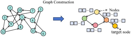
Figure 1.
As illustrated in the figure, a time-evolving adjacency structure is constructed by computing correlation coefficients between historical signal sequences over a sliding window. Each node represents an independent signal, and the edge weights reflect the degree of inter-signal correlation. This dynamic graph is then input into a graph attention module to extract structure-aware embeddings, which enhance the capacity of the model to capture interactions across heterogeneous signal modalities.
Through the graph attention mechanism, structural embeddings for each asset are generated. Concurrently, the temporal sequence of each asset is modeled via three Transformer branches corresponding to short-term, mid-term, and long-term temporal windows, enabling the extraction of multi-scale temporal trends. The macroeconomic factor module integrates structured economic indicators with sentiment representations derived from policy texts, aligning them with market behavior through attention mechanisms to generate macro-level disturbance embeddings. The outputs from the three modules are then concatenated and passed into the prediction network to jointly forecast both the direction and magnitude of future returns. This architecture enables collaborative modeling of structural information, temporal dynamics, and external factors, contributing to enhanced robustness and practical applicability.
3.3.1. Graph Modeling and Graph Attention Module
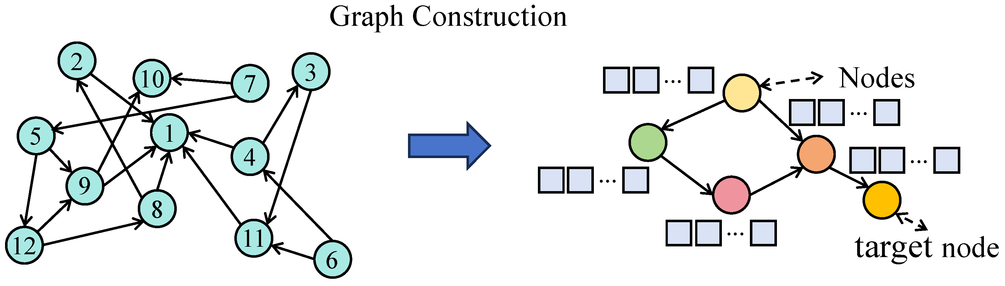
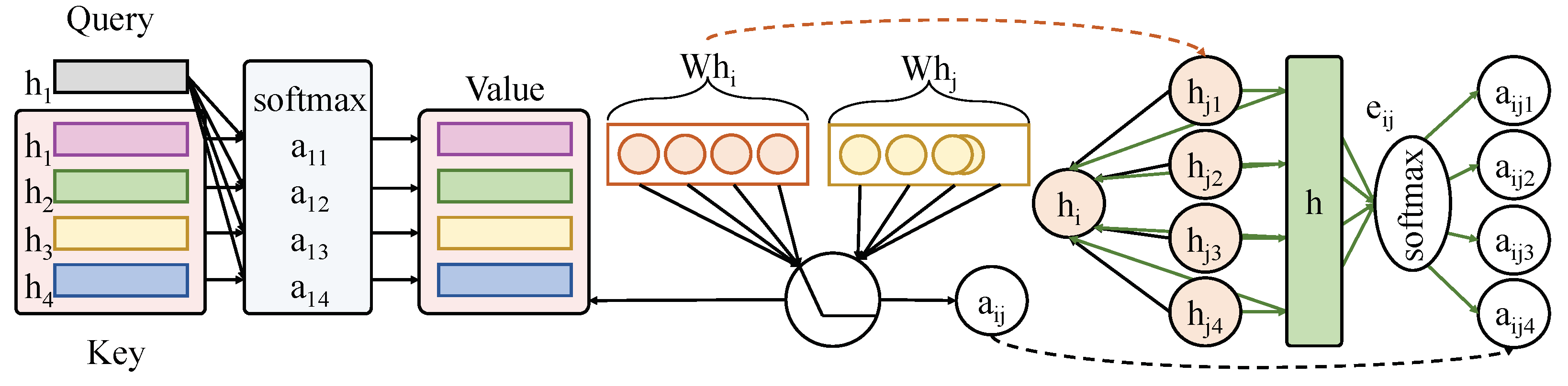
This module is designed to capture structured relationships among signal nodes. As illustrated in Figure 2, each node receives an initial feature vector , which encodes raw observations and derived descriptors of signal i. These inputs are linearly projected via a transformation matrix W to produce embedded vectors .

Figure 2.
The figure illustrates the construction of a graph based on inter-signal correlation and the computation process of attention weights within the Graph Attention Network. Each node receives an initial feature vector , which is transformed via a learnable weight matrix W to obtain embeddings. Attention scores are computed using a shared parameter vector a for each pair of neighboring nodes, then normalized to produce attention weights . The updated embedding is obtained through a weighted sum of neighboring node features, modulated by .
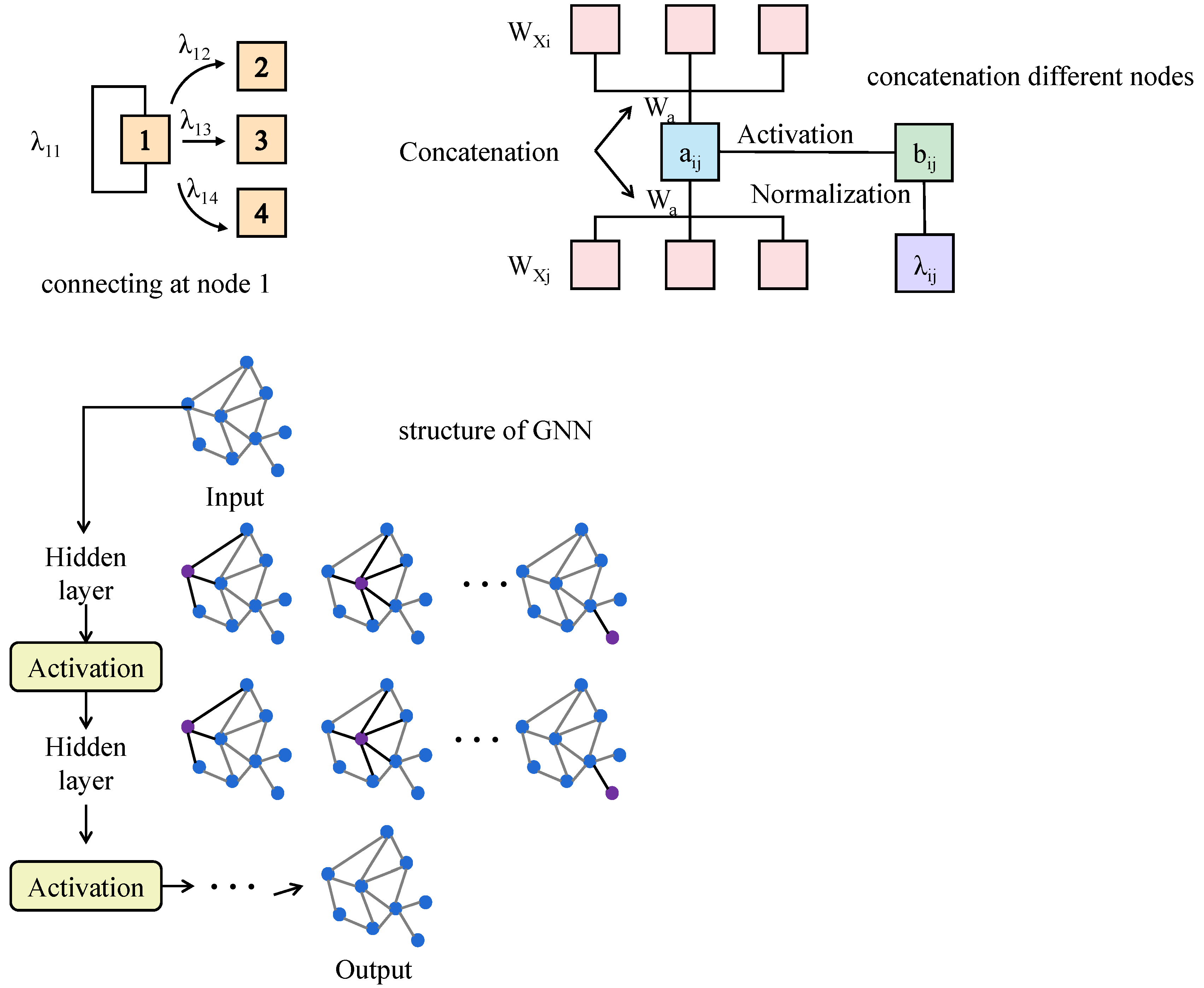
For a given node i and its neighbor j, the attention coefficient is computed using a shared attention vector a:
Here, denotes vector concatenation. The attention score is then normalized across all neighbors using the Softmax function to obtain the final attention weight :
Here, visually represents the edge weight from node j to node i, quantifying the influence of node j in updating node i’s representation. The updated embedding for node i is then obtained by a weighted aggregation of neighbor features:
where is a non-linear activation function (ReLU in this study). A multi-head attention mechanism performs this operation in parallel, with several independent attention heads. The results are aggregated via concatenation or averaging, forming the unified output representation. A three-layer stacked GAT is employed to progressively incorporate high-order neighborhood information. The structure graph itself is dynamically updated at each time step using a sliding correlation window, and edge connections are established based on inter-signal correlation measures. The final graph-based structural embeddings are concatenated with the outputs of the temporal and semantic modules for joint modeling in the signal forecasting task.
3.3.2. Multi-Scale Transformer Module (Revised)
To capture dynamic patterns across different temporal resolutions, a multi-scale Transformer module is constructed consisting of three parallel encoder branches. As illustrated in Figure 3, each branch independently processes temporal input sequences of different lengths, corresponding to short-term (5 steps), mid-term (20 steps), and long-term (60 steps) segments. This architecture enables the simultaneous modeling of transient fluctuations and persistent trends.
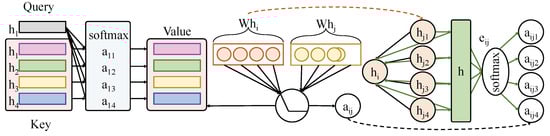
Figure 3.
The module consists of three parallel Transformer encoder branches, each dedicated to processing input sequences of different temporal lengths: short-term (5 steps), mid-term (20 steps), and long-term (60 steps). Each branch includes two stacked Transformer layers for extracting temporal features at its respective resolution. The internal computation of the multi-head self-attention mechanism is illustrated, including the linear transformations for query (Q), key (K), and value (V), and the computation of attention weights . Outputs from the three branches are pooled into vectors , , and , which are then fused through a gating mechanism to form the final temporal representation .
The full input sequence is first split into three sub-sequences: for short-term, for mid-term, and for long-term encoding. These are passed into three structurally identical Transformer encoder branches, each composed of two stacked Transformer layers. Each Transformer layer contains two subcomponents: a multi-head self-attention mechanism and a position-wise feedforward network, augmented with residual connections and LayerNorm for stability. For each time step t, the input is projected into three spaces: query (), key (), and value (), where , , and are learnable matrices. The attention score between time steps i and j is computed as
The normalized attention weights are used to aggregate values:
This attention process is performed independently in all three branches. The outputs of each branch are then pooled via average pooling to obtain fixed-size temporal representations, denoted as (short-term), (mid-term), and (long-term), respectively. These representations are then fused via a learnable gating mechanism to produce the final temporal encoding :
Here, , , and are learnable transformation matrices; b is a bias term; and denotes the ReLU activation function. This module offers two primary advantages. First, the use of three distinct temporal windows enables the extraction of behavioral features at multiple resolutions, addressing the fixed-window limitations of conventional Transformers. Second, the gating mechanism adaptively weights each timescale’s contribution based on the current input, enhancing the model’s robustness to variations in temporal dynamics. The resulting is subsequently concatenated with the structural and semantic representations for downstream prediction. This module significantly improves the capacity of the overall system to model non-stationary, multiscale temporal signals, particularly in environments exhibiting both volatility and persistent macro trends.
3.3.3. Macroeconomic Factor Fusion Module
The macroeconomic factor fusion module is designed to incorporate external economic environments and policy expectations into the quantitative signal generation framework, addressing the limitations of conventional models in capturing macro-level disturbances. This module consists of two parallel pathways: one for structured macroeconomic variables and another for unstructured policy semantics. The former captures quantifiable indicators such as GDP growth, CPI, and interest rates, while the latter leverages a language model to extract sentiment and semantic representations from policy-related news texts, reflecting potential directional influences on market dynamics. To enable the integration of these heterogeneous sources, a dual-branch embedding network is constructed, and an attention-based fusion mechanism is employed to dynamically align macro factors with temporal market features, thereby enhancing the model’s adaptability to economic shifts. In the structured pathway, the input consists of nine time-aligned macroeconomic indicators, denoted as . This vector is processed by a three-layer feedforward network to perform dimensional expansion and nonlinear transformation, resulting in a structured macro embedding . The network comprises hidden layers of sizes 32, 64, and 64, respectively, and applies ReLU activations and dropout regularization with a rate of 0.2 to prevent overfitting. The transformation process is defined as
Simultaneously, in the unstructured pathway, daily policy-related news texts are submitted to the GPT-4 API for semantic analysis, producing a sentiment score and a category distribution vector , where represents predefined policy categories (including monetary, fiscal, regulatory, industrial guidance, external shocks, and others). These outputs are concatenated into a 7-dimensional vector and processed by a two-layer neural network to generate the unstructured macro embedding , as follows:
The two embeddings are then fused using a gated weighting mechanism to produce a unified macro representation . The fusion weight is derived from the structured pathway, calculated as
Here, denotes the sigmoid activation function, ensuring that the fusion coefficient remains within the range . This design enables the structured indicators to dominate under stable conditions, while allowing the model to shift attention toward policy semantics under conditions of strong sentiment-driven shocks, thereby achieving adaptive macro fusion. The fused macro representation is subsequently integrated with the temporal embedding from the temporal modeling module through a cross-attention mechanism. Specifically, is used as the query vector, while the temporal embedding serves as the key and value. The attention process is computed as
where are the transformation matrices. This mechanism guides temporal representations to align with macro-level signals by re-weighting asset-specific time features based on external economic context. The updated temporal embeddings are then combined with the graph-based structural embeddings for final model input fusion. This module offers several distinct advantages. By explicitly modeling both structured and unstructured macroeconomic pathways, it captures not only trend-level signals from standard indicators but also sentiment and expectation-driven components from policy texts. This dual representation becomes particularly valuable during periods of heightened uncertainty or major policy transitions, where external shocks significantly influence system behavior. Furthermore, the use of attention-based alignment with temporal embeddings enables fine-grained control over the influence of macro signals on asset-level time segments, enhancing both prediction accuracy and individual asset interpretability. This heterogeneous multi-source fusion strategy substantially improves the economic interpretability and robustness of the model, thereby providing a strong foundation for the deployment of adaptive HFT strategies.
3.3.4. Unified Optimization Objective for Multi-Module Coordination
To further strengthen the coordination among modules, a unified optimization objective is introduced into the training framework. Instead of relying solely on feature concatenation and attention mechanisms, the proposed method jointly trains the structural, temporal, and macroeconomic modules under a shared loss function. Specifically, the total objective combines three components: the classification loss , the regression loss , and a semantic alignment loss that ensures consistency between macroeconomic representations and temporal embeddings. The overall formulation is as follows:
where and are trade-off hyperparameters. This joint training strategy enables cross-module gradient propagation and collaborative representation learning. The empirical results presented in Section 4.9 demonstrate that the unified objective improves not only the convergence stability but also forecasting accuracy, confirming the effectiveness of the proposed integration enhancement.
4. Results and Discussion
4.1. Experimental Design
In the experimental design, a hierarchical backtesting window approach was adopted to ensure that the evaluation of the model reflected true predictive capability on unseen future data. Specifically, the full time series spanning from 2014 to 2023 was split chronologically into three phases: a training set, validation set, and test set. The training set, comprising 70% of the data, was used for model fitting; the validation set, accounting for 15%, was utilized for hyperparameter tuning and early stopping; and the remaining 15% was reserved as the test set to evaluate the generalization ability on out-of-sample data. Let the total length of the dataset be T, then the training interval has a length of , the validation interval is , and the test interval is , with and . In terms of prediction granularity, this study focused on generating signals at a daily frequency, where an input sample was constructed each day to forecast either the next day’s or the next week’s return direction or value. A sliding window mechanism was implemented to extract continuous historical observations of length w as model input, and the target variable was the return steps ahead. Given a current timestamp t, the input sequence is denoted as and the prediction target is , where indicates one-day-ahead forecasting and corresponds to one-week-ahead forecasting. The sliding window ensures that every training and prediction iteration is based on the most recently available data, thereby aligning with real-world decision-making logic, while improving sample efficiency. This approach enhanced the model’s ability to learn temporal dependencies and pattern evolutions in the sequence data, ensuring that the experimental process remained rigorous and that the evaluation outcomes were reliable and practically relevant.
4.2. Evaluation Metrics
To comprehensively evaluate the model’s performance in the signal prediction task, two types of metrics were used: classification metrics for direction prediction, and regression metrics for return value forecasting. The classification metrics included Precision, Recall, and F1-Score, which assessed the model’s accuracy and completeness in identifying directional signals. In addition, regression performance was evaluated using Mean Squared Error (MSE) and Mean Absolute Error (MAE), which reflect the deviation between predicted and actual signal magnitudes.
Here, denotes true positives, false positives, false negatives, the observed value, the predicted value, and N the number of samples. These metrics jointly captured the model’s effectiveness in both directional classification and magnitude estimation, thus offering a comprehensive assessment of predictive quality.
4.3. Baseline Models
This study incorporated seven representative baseline algorithms for comparative evaluation: SVM [27], XGBoost [28], LightGBM [29], LSTM [30], TCN [31], FinBERT [32], and StockGCN [33]. SVM is a classic supervised learning algorithm that performs well in high-dimensional, small-sample settings. XGBoost and LightGBM, as gradient boosting tree models, are known for strong feature selection and nonlinear modeling capabilities. LSTM is suited for temporal data, capturing long-range dependencies and trends. TCN uses one-dimensional causal convolutions to model sequence structure more efficiently than recurrent architectures. FinBERT, a domain-adapted pretrained language model, can extract fine-grained sentiment signals from policy texts or narratives. StockGCN applies graph convolution to model structural relationships and dynamic interactions across multiple entities. Together, these models span traditional machine learning, deep sequence modeling, semantic feature extraction, and relational representation learning, forming a robust benchmark for evaluating the proposed method’s effectiveness.
4.4. Classification and Regression Results on Signal Sequences
This experiment was designed to evaluate the performance differences across various types of models in handling high-frequency signal sequence classification and continuous-value prediction tasks, aiming to assess the proposed framework in terms of accuracy, stability, and error control. The task is inherently a multivariate nonlinear time series analysis problem, characterized by structural complexity, frequent fluctuations, and multi-scale interactions. Therefore, an effective model is expected to balance local feature extraction, long-range dependency modeling, and multi-source information integration. Comparative experiments were conducted using traditional machine learning models (SVM, XGBoost, LightGBM), deep sequence models (LSTM, TCN), pre-trained semantic models (FinBERT), structure-aware graph models (StockGCN), and the proposed multimodal modeling framework.
As shown in Table 2, in terms of classification metrics, the traditional models generally achieved precisions between 81% and 83%. With enhanced sensitivity to temporal sequences, models such as LSTM and TCN achieved precisions exceeding 85%. FinBERT, equipped with capabilities for processing unstructured semantic information, exhibited a notable advantage in signal discrimination. StockGCN, by modeling graph-based structural relationships, demonstrated improved stability in handling high-frequency feature variations. The proposed method outperformed all baseline models across all metrics, achieving a precision of 92.4% and an F1-score of 92.0%, indicating a systematic improvement in overall signal modeling capabilities. From the perspective of model architecture, traditional models such as SVM, relying on static hyperplane separation, are limited in capturing dynamic temporal patterns, resulting in suboptimal recall and F1 performance. While tree-based models like XGBoost and LightGBM can fit complex feature relationships, they exhibit structural limitations in modeling temporal dependencies, leading to challenges in responding to high-frequency volatility. In contrast, LSTM introduces long-term memory capabilities through gated mechanisms, significantly enhancing sequential modeling. TCN further replaces recurrent operations with 1D convolutions, improving parallelism and capturing long-range dependencies, which proves beneficial for continuous signal prediction. FinBERT, utilizing multi-layer Transformer structures, offers inherent advantages in processing external textual signals. StockGCN captures inter-signal structural correlations through graph convolution operations over topological asset relations, making it suitable for modeling high-frequency interactions among multiple entities. The proposed method builds upon these strengths by integrating a graph attention mechanism, multi-scale Transformer encoding, and macro-semantic embeddings generated by LLMs. Through three-path representation learning and a unified fusion layer, the framework enables joint modeling across structural, temporal, and external semantic dimensions. This holistic design enhances the model’s capability in perceiving nonlinear signal behavior, multi-dimensional dependencies, and heterogeneous information. As a result, the framework demonstrated superior adaptability and robustness, supporting more accurate and stable predictions under complex signal environments.
Table 2.
Classification and regression results on signal sequences.
4.5. Performance Comparison Under Module Removal Settings
This experiment was designed to analyze the independent contributions of each sub-module within the proposed multi-module deep architecture, specifically evaluating the roles and relative importance of temporal modeling, graph-based structural modeling, and macro-level perturbation modeling. By sequentially removing each of the three core modules and comparing the resulting performance changes in both classification and regression tasks with respect to the complete model, the criticality of each module in high-dimensional signal processing could be quantitatively assessed. This experiment constituted a classical structural ablation test, whose underlying objective was to examine the marginal contribution of distinct information dimensions—such as temporal dependency, spatial structure, and external semantics—to the overall predictive performance within a complex modeling framework.
As shown in Table 3, the complete model achieved the highest scores across all evaluation metrics, with a precision of 92.4%, a recall of 91.6%, and an F1-score of 92.0%. The removal of any of the three modules led to a measurable performance degradation, with the most significant decline observed when the temporal modeling module was excluded, where the F1-score dropped to 87.2. This indicates a substantial reduction in the model’s ability to capture dynamic signal evolution. From a theoretical modeling perspective, the three sub-modules undertake complementary signal processing tasks with distinct functional emphases. The graph module introduces non-Euclidean adjacency structures by constructing relational graphs among entities, effectively capturing interdependencies between input signals, such as co-movement patterns across assets, features, or observational units in historical data. By aggregating node features within local neighborhoods, this module maintains structural consistency, enabling stable representation of hierarchical changes, even in high-dimensional settings. The macro module, on the other hand, encodes low-frequency external perturbations by transforming policy changes and macroeconomic shifts into sentiment vectors that are fused with internal signal dynamics. Although its direct impact on performance is less pronounced than the graph module, it substantially enhances the model’s robustness during disruptive events or periods of elevated uncertainty. The temporal module serves as the backbone of the overall sequence modeling pipeline. It is responsible for capturing dynamic temporal dependencies and multi-scale evolution patterns. Leveraging a Transformer-based architecture, this module offers superior global context perception and high-dimensional parallel modeling compared to traditional RNN or convolutional approaches. The most significant performance drop observed when this module was removed underscores its critical role in representing the temporal characteristics of signals, which are fundamental to the model’s predictive capabilities. From a mathematical modeling standpoint, the graph module introduces spatial correlation learning, the macro module provides conditional perturbation modeling, and the temporal module governs the encoding of global dynamic trajectories. Together, they form a multi-dimensional, mutually enhancing architecture that enables robust and accurate predictions across diverse and complex signal environments.
Table 3.
Performance comparison under module removal settings.
4.6. Strategy Performance Comparison Under Different Data Environments
This experiment was designed to evaluate the robustness and adaptability of the proposed multi-module signal modeling framework under varying data conditions. Specifically, three distinct scenarios were considered: a stable growth phase, a high-frequency volatility phase, and an overall declining phase. These settings were used to assess the model’s predictive accuracy and error control capabilities across diverse temporal dynamics. The core objective of this experiment was to examine the model’s ability to perceive non-stationary distributions, recover from localized disturbances, and accurately represent complex dynamic trajectories.
As shown in Table 4, the model achieved the highest performance during the stable growth phase, with an F1-score of 93.1 and precision and recall reaching 93.5% and 92.7%, respectively. During the high-frequency volatility phase, the performance experienced a slight decline but remained above 91% across all classification metrics. In the overall declining phase, a further decrease in performance was observed, with the F1-score falling to 89.7 and a corresponding increase in error metrics. Nonetheless, the proposed framework consistently outperformed traditional architectures under all conditions. From the perspective of big data modeling and signal analysis, these results highlight the structural advantages of the multi-module collaborative framework in modeling nonlinear and non-stationary signals. In stable growth conditions characterized by strong trend dominance, signal structures exhibit high predictability. The multi-scale temporal modeling module effectively captures dominant frequencies and persistence, while the graph structure module can learn relatively stable inter-node dependencies, resulting in optimal performance. In the high-frequency volatility phase, where short-term perturbations and long-term trends are intertwined, the temporal module mitigates transient disturbances via multi-scale encoding. However, graph edge weights fluctuate more frequently, and the contribution of low-frequency macro factors is less pronounced in this context, leading to a slight but controlled performance drop. In contrast, during the overall declining phase, signals demonstrate more pronounced nonlinearity and abrupt transitions, such as sharp downturns and heavy-tailed noise. In such settings, the temporal module faces greater challenges due to elevated forecasting bias, and the volatility of graph adjacency structures diminishes the effectiveness of structural dependencies. Notably, the macro module, through the integration of semantic-level priors, provides critical resilience against such disruptions by compensating for local information loss and stabilizing predictions. Collectively, the findings from this experiment confirm the structural adaptability and noise resistance of the proposed heterogeneous multi-path framework when exposed to complex and variable input signals. The model demonstrates broad applicability and resilience in real-world deployments involving diverse data conditions.
Table 4.
Strategy performance comparison under different market conditions.
4.7. Impact of Input Frequency Features on Model Performance
This experiment was designed to assess the impact of features with different frequency resolutions on the overall performance in signal modeling and forecasting tasks, with the aim of validating the necessity and effectiveness of multi-frequency feature fusion in multi-scale sequence modeling. In complex system signal processing, low-frequency features typically reflect long-term trends and macro-level system behavior, while high-frequency features capture rapid short-term fluctuations and detailed changes. These two types of signals are inherently complementary. To empirically investigate this complementarity, three input configurations were constructed: low-frequency only, high-frequency only, and fused low- and high-frequency features. Each was fed into a unified model architecture to evaluate the classification and regression performance.
As shown in Table 5, the model using low-frequency features alone achieved an F1-score of 87.9%, while the high-frequency-only configuration slightly improved the performance to 89.2%. The multi-frequency fusion model achieved the best results, with a precision of 92.4% and an F1-score of 92.0%, accompanied by significant reductions in error metrics such as MSE and MAE. These findings demonstrate that the structural hierarchy of feature frequency significantly influences modeling outcomes, and that multi-scale information fusion provides measurable benefits in handling non-stationary sequences. From a mathematical modeling perspective, this performance pattern can be attributed to the distinct representational roles of signals across frequency domains. Low-frequency features, being more stationary and trend-oriented, are critical for modeling long-term dependencies and establishing stable prediction baselines. However, reliance on low-frequency inputs alone limits the model’s responsiveness to short-term disturbances or abrupt changes, often resulting in temporal lag in high-volatility scenarios. In contrast, high-frequency features offer superior temporal resolution and volatility sensitivity, enabling finer-grained pattern recognition and detection of transient anomalies. Nevertheless, their high variability also makes them more susceptible to noise, and in the absence of contextual constraints or trend anchoring, they tend to induce overfitting or localized prediction errors. The integration of low- and high-frequency features enables the model to balance global stability and local sensitivity, thus enhancing the expressive capacity of signal representation. Within the network architecture, this fusion is realized through mechanisms such as multi-scale temporal windows, shared weights, and attention-based cross-resolution alignment, allowing for joint perception and distributed modeling across frequency bands. As evidenced by the results, the fused model not only outperformed the other models in classification accuracy but also demonstrated lower prediction errors, indicating its superiority in capturing sequence distributions and modeling dynamic responses. These findings further support the critical role of multi-frequency fusion in complex sequence modeling tasks and provide structural justification for the development of temporally adaptive modeling systems.
Table 5.
Impact of different frequency feature inputs on model performance.
4.8. Parameter and Activation Sensitivity Analysis
To comprehensively evaluate the model’s stability and convergence under varying configurations, a dual-dimensional sensitivity analysis was conducted, focusing on the learning rate and the activation function. For learning rate analysis, four initial values were tested: . With all other settings held constant, the evolution of training loss and validation F1-score was monitored. The results show that the model maintained stable performance when the learning rate was within the range of to , with F1-score fluctuations less than 1.5%. This indicates that the proposed method exhibited strong robustness with respect to optimizer parameter selection. In addition, an activation function substitution experiment was performed by replacing the standard ReLU function with SmoothReLU [34], a smooth, globally differentiable activation defined as . Incorporating SmoothReLU across all neural units led to improved convergence behavior, reducing the number of training epochs required by 5 to 10. Furthermore, the final F1-score on the validation set increased by approximately 0.6%. These findings demonstrate that SmoothReLU not only mitigates the dead neuron problem but also enhances training stability and generalization capability. This analysis confirmed the framework’s adaptability to hyperparameter configurations and activation design, supporting its applicability in complex, high-frequency prediction scenarios.
4.9. Limitations and Future Work
Despite the proposed high-frequency signal generation framework demonstrating superior performance across multiple evaluation metrics and exhibiting strong stability and adaptability under various market conditions, several limitations remain that warrant further investigation. The current macro factor modeling mechanism incorporates policy sentiment vectors extracted via language models; however, it does not fully exploit high-frequency unstructured textual sources such as social media feeds, analyst reports, and real-time news streams. Future work could integrate reinforcement learning or online learning approaches, where strategy backtesting feedback could be introduced as a reward signal to construct a dynamic update mechanism, thereby enhancing the robustness of returns and the effectiveness of risk control. On the other hand, although the current model integrates structured graph modeling, multi-scale temporal encoding, and semantic macro factor modeling, the interactions among these modules are primarily based on simple feature concatenation and attention mechanisms. A tighter coupling of components through joint optimization has yet to be established. Subsequent research could explore joint module training and collaborative attention mechanisms to further enhance the coherence and interpretability of the overall framework.
5. Conclusions
This study proposed a deep learning framework for high-frequency signal forecasting that integrates structural modeling, cross-scale temporal encoding, and macro-level semantic modeling. Structural relationships among signals are captured via graph neural networks, while a multi-scale Transformer architecture extracts behavioral patterns at short-, mid-, and long-term horizons. In addition, macroeconomic policy texts are processed using LLMs to generate semantic embeddings, which enhance the system’s sensitivity to external shocks. These three representations are fused within a unified architecture to support end-to-end signal modeling and forecasting. The experimental results demonstrate that the proposed method outperformed seven strong baseline models—including LSTM, TCN, FinBERT, and StockGCN—in both classification and regression tasks. The framework achieved higher accuracy, better generalization, and greater robustness. Ablation studies further confirmed the independent contributions of each module, particularly the structural modeling and semantic alignment mechanisms in improving predictive stability. The scientific contributions of this work are fourfold: (1) a unified framework integrating structural, temporal, and semantic paths; (2) a multi-scale parallel Transformer design that enhances the modeling of non-stationary dynamics; (3) the first incorporation of LLM outputs for macro-level signal conditioning; and (4) the implementation of a deployable, automated forecasting system. The current model still relies on simple concatenation and attention mechanisms for interactions between modules, which may lead to limited coordination. Future research could explore reinforcement learning-based feedback or multi-task prediction structures to further improve adaptability and risk-awareness in high-frequency environments.
Author Contributions
Conceptualization, X.Z., L.Z., S.H., Y.H. and C.L.; Data curation, Y.H. and H.Y.; Formal analysis, T.L. and Y.J.; Funding acquisition, C.L.; Investigation, Y.J. and H.Y.; Methodology, X.Z., L.Z. and S.H.; Project administration, C.L.; Resources, Y.H. and H.Y.; Software, X.Z., L.Z., S.H. and T.L.; Supervision, C.L.; Validation, Y.J.; Visualization, T.L. and H.Y.; Writing—original draft, X.Z., L.Z., S.H., T.L., Y.H., Y.J. and C.L.; X.Z., L.Z., S.H. and T.L. contributed equally to this work. All authors have read and agreed to the published version of the manuscript.
Funding
This research was funded by National Natural Science Foundation of China grant number 61202479.
Data Availability Statement
The data presented in this study are available on request from the corresponding author.
Conflicts of Interest
The authors declare no conflicts of interest.
References
- Goldstein, I. Information in financial markets and its real effects. Rev. Financ. 2023, 27, 1–32. [Google Scholar] [CrossRef]
- Eaton, G.W.; Green, T.C.; Roseman, B.; Wu, Y. Zero-Commission Individual Investors, High Frequency Traders, and Stock Market Quality. 2021. Available online: https://pages.stern.nyu.edu/~jhasbrou/SternMicroMtg/Old/SternMicroMtg2021/Papers/Zero-commission%20individual%20traders.pdf (accessed on 19 March 2021).
- Fu, Y. GM (1,1) and Quantitative Trading Decision Model. In Financial Engineering and Risk Management; Springer: Berlin/Heidelberg, Germany, 2022. [Google Scholar]
- Lin, Z.F.; Zhao, H.H.; Sun, Z. Nonlinear modeling of financial state variables and multiscale numerical analysis. Eur. Phys. J. Spec. Top. 2025, 7, 1–15. [Google Scholar] [CrossRef]
- Xie, C.; Zhang, Y.; Wang, M.; Liu, Z. Quantamental Trading: Fundamental and Quantitative Analysis with Multi-factor Regression Model Strategy. In Proceedings of the International Conference on Business and Policy Studies; Springer: Singapore, 2023; pp. 1455–1470. [Google Scholar]
- Eti, S. The use of quantitative methods in investment decisions: A literature review. Res. Anthol. Pers. Financ. Improv. Financ. Lit. 2021, 1–20. [Google Scholar] [CrossRef]
- Olukoya, O. Time series-based quantitative risk models: Enhancing accuracy in forecasting and risk assessment. Int. J. Comput. Appl. Technol. Res. 2023, 12, 29–41. [Google Scholar]
- Zhang, J.; Huang, Y.; Huang, C.; Huang, W. Research on arima based quantitative investment model. Acad. J. Bus. Manag. 2022, 4, 54–62. [Google Scholar]
- Diqi, M.; Utami, E.; Wibowo, F.W. A Study on Methods, Challenges, and Future Directions of Generative Adversarial Networks in Stock Market Prediction. In Proceedings of the 2024 IEEE International Conference on Technology, Informatics, Management, Engineering and Environment (TIME-E), Bali, Indonesia, 7–9 August 2024; Volume 5, pp. 148–153. [Google Scholar]
- Sahu, S.K.; Mokhade, A.; Bokde, N.D. An overview of machine learning, deep learning, and reinforcement learning-based techniques in quantitative finance: Recent progress and challenges. Appl. Sci. 2023, 13, 1956. [Google Scholar] [CrossRef]
- Ludkovski, M. Statistical machine learning for quantitative finance. Annu. Rev. Stat. Its Appl. 2023, 10, 271–295. [Google Scholar] [CrossRef]
- Liu, X.Y.; Yang, H.; Gao, J.; Wang, C.D. FinRL: Deep reinforcement learning framework to automate trading in quantitative finance. In Proceedings of the Second ACM International Conference on AI in Finance, Virtual Event, 3–5 November 2021; pp. 1–9. [Google Scholar]
- Horvath, B.; Muguruza, A.; Tomas, M. Deep learning volatility: A deep neural network perspective on pricing and calibration in (rough) volatility models. Quant. Financ. 2021, 21, 11–27. [Google Scholar] [CrossRef]
- Khunger, A. Learning for financial stress testing: A data-driven approach to risk management. Int. J. Innov. Stud. 2022, 3, 97–113. [Google Scholar] [CrossRef]
- Sirignano, J.; Cont, R. Universal features of price formation in financial markets: Perspectives from deep learning. In Machine Learning and AI in Finance; Routledge: London, UK, 2021; pp. 5–15. [Google Scholar]
- Nguyen, D.K.; Sermpinis, G.; Stasinakis, C. Big data, artificial intelligence and machine learning: A transformative symbiosis in favour of financial technology. Eur. Financ. Manag. 2023, 29, 517–548. [Google Scholar] [CrossRef]
- Khuwaja, P.; Khowaja, S.A.; Dev, K. Adversarial learning networks for FinTech applications using heterogeneous data sources. IEEE Internet Things J. 2021, 10, 2194–2201. [Google Scholar] [CrossRef]
- Borisov, V.; Broelemann, K.; Kasneci, E.; Kasneci, G. DeepTLF: Robust deep neural networks for heterogeneous tabular data. Int. J. Data Sci. Anal. 2023, 16, 85–100. [Google Scholar] [CrossRef]
- Liu, Q.; Zhang, Y.; Wei, J.; Wu, H.; Deng, M. HLSTM: Heterogeneous long short-term memory network for large-scale InSAR ground subsidence prediction. IEEE J. Sel. Top. Appl. Earth Obs. Remote Sens. 2021, 14, 8679–8688. [Google Scholar] [CrossRef]
- Ahmed, I.; Ahmad, M.; Chehri, A.; Jeon, G. A heterogeneous network embedded medicine recommendation system based on LSTM. Future Gener. Comput. Syst. 2023, 149, 1–11. [Google Scholar] [CrossRef]
- Qu, L.; Zhou, Y.; Liang, P.P.; Xia, Y.; Wang, F.; Adeli, E.; Fei-Fei, L.; Rubin, D. Rethinking architecture design for tackling data heterogeneity in federated learning. In Proceedings of the IEEE/CVF Conference on Computer Vision and Pattern Recognition, New Orleans, LA, USA, 18–24 June 2022; pp. 10061–10071. [Google Scholar]
- Corso, G.; Stark, H.; Jegelka, S.; Jaakkola, T.; Barzilay, R. Graph neural networks. Nat. Rev. Methods Prim. 2024, 4, 17. [Google Scholar] [CrossRef]
- Brody, S.; Alon, U.; Yahav, E. How attentive are graph attention networks? arXiv 2021, arXiv:2105.14491. [Google Scholar]
- Tumiran, M.A. Constructing a framework from quantitative data analysis: Advantages, types and innovative approaches. Quantum J. Soc. Sci. Humanit. 2024, 5, 198–212. [Google Scholar] [CrossRef]
- Peng, R.; Liu, K.; Yang, P.; Yuan, Z.; Li, S. Embedding-based retrieval with llm for effective agriculture information extracting from unstructured data. arXiv 2023, arXiv:2308.03107. [Google Scholar]
- De Bellis, A. Structuring the Unstructured: An LLM-Guided Transition. In Proceedings of the Doctoral Consortium at ISWC 2023 Co-Located with 22nd International Semantic Web Conference (ISWC 2023), Athens, Greece, 7 November 2023. [Google Scholar]
- Cortes, C.; Vapnik, V. Support-vector networks. Mach. Learn. 1995, 20, 273–297. [Google Scholar] [CrossRef]
- Chen, T.; Guestrin, C. Xgboost: A scalable tree boosting system. In Proceedings of the 22nd ACM Sigkdd International Conference on Knowledge Discovery and Data Mining, San Francisco, CA, USA, 13–17 August 2016; pp. 785–794. [Google Scholar]
- Ke, G.; Meng, Q.; Finley, T.; Wang, T.; Chen, W.; Ma, W.; Ye, Q.; Liu, T.Y. Lightgbm: A highly efficient gradient boosting decision tree. Adv. Neural Inf. Process. Syst. 2017, 30, 193–209. [Google Scholar]
- Hochreiter, S.; Schmidhuber, J. Long short-term memory. Neural Comput. 1997, 9, 1735–1780. [Google Scholar] [CrossRef] [PubMed]
- Bai, S.; Kolter, J.Z.; Koltun, V. An empirical evaluation of generic convolutional and recurrent networks for sequence modeling. arXiv 2018, arXiv:1803.01271. [Google Scholar]
- Araci, D. Finbert: Financial sentiment analysis with pre-trained language models. arXiv 2019, arXiv:1908.10063. [Google Scholar]
- Xin, C.; Han, Q.; Pan, G. Correlation Matters: A Stock Price Predication Model Based on the Graph Convolutional Network. In International Conference on Intelligent Computing; Springer: Berlin/Heidelberg, Germany, 2024; pp. 228–239. [Google Scholar]
- Vladov, S.; Scislo, L.; Sokurenko, V.; Muzychuk, O.; Vysotska, V.; Osadchy, S.; Sachenko, A. Neural Network Signal Integration from Thermogas-Dynamic Parameter Sensors for Helicopters Turboshaft Engines at Flight Operation Conditions. Sensors 2024, 24, 4246. [Google Scholar] [CrossRef]
Disclaimer/Publisher’s Note: The statements, opinions and data contained in all publications are solely those of the individual author(s) and contributor(s) and not of MDPI and/or the editor(s). MDPI and/or the editor(s) disclaim responsibility for any injury to people or property resulting from any ideas, methods, instructions or products referred to in the content. |
© 2025 by the authors. Licensee MDPI, Basel, Switzerland. This article is an open access article distributed under the terms and conditions of the Creative Commons Attribution (CC BY) license (https://creativecommons.org/licenses/by/4.0/).