A Study on the Seismic Performance of Steel H-Column and T-Beam-Bolted Joints

Abstract
:1. Introduction
2. Establishment and Verification of Model
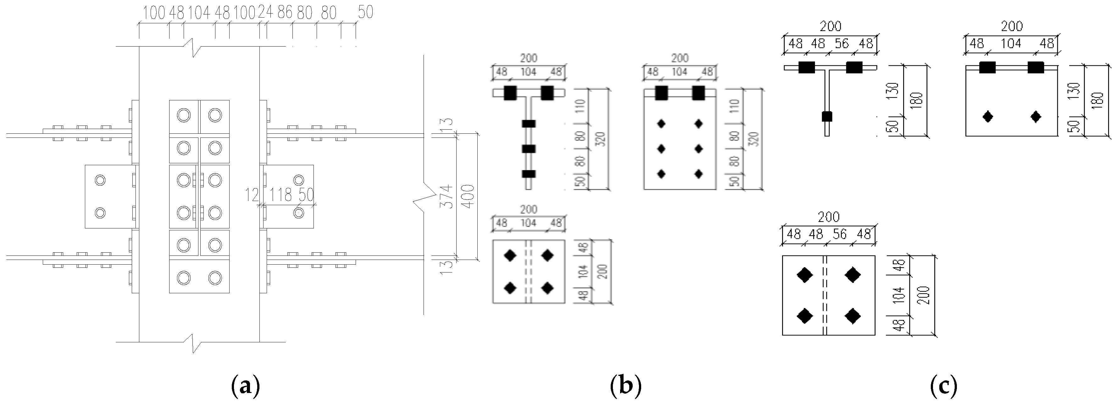
2.1. Node Size
2.2. Model Building
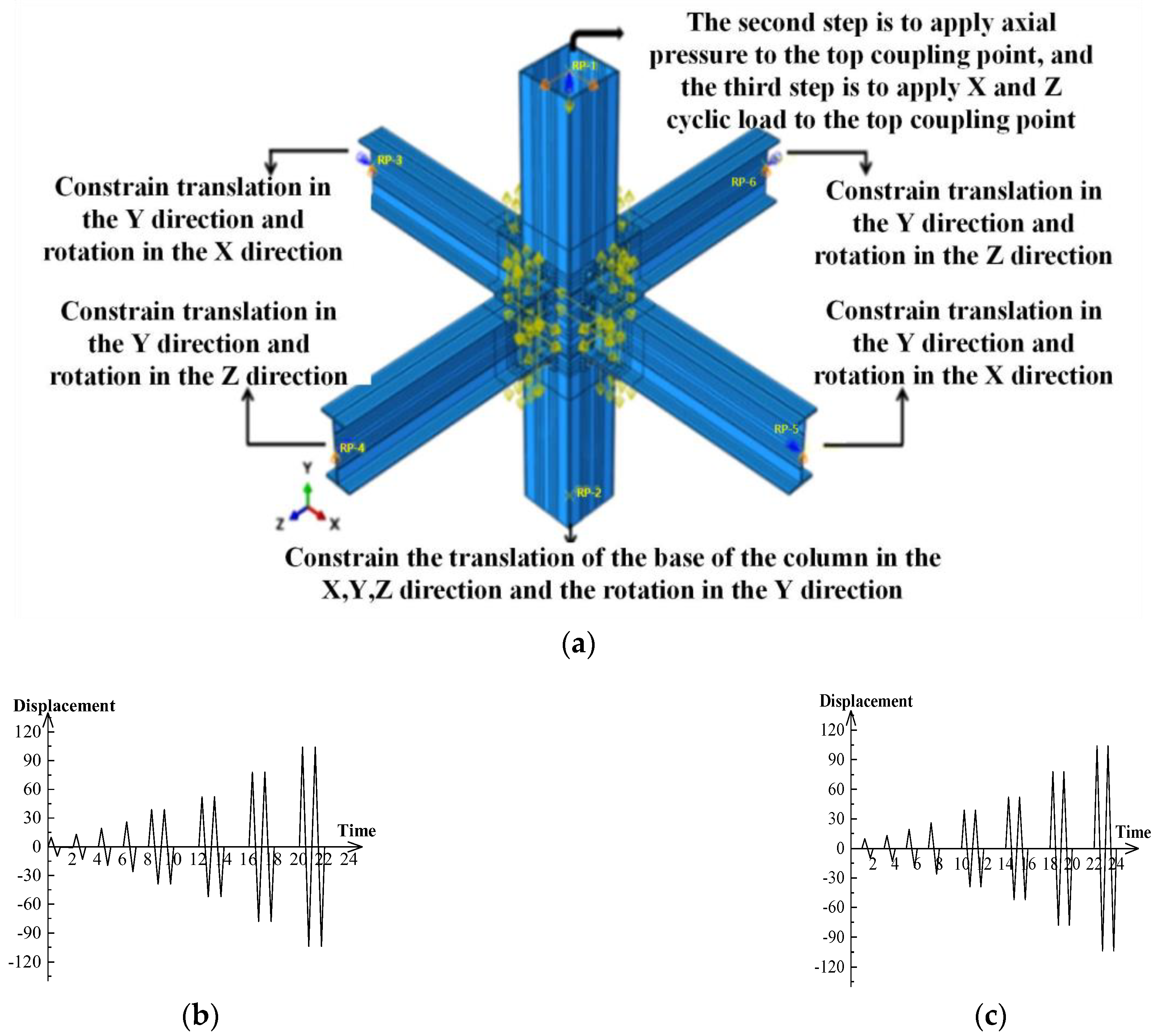
2.3. Boundary Condition
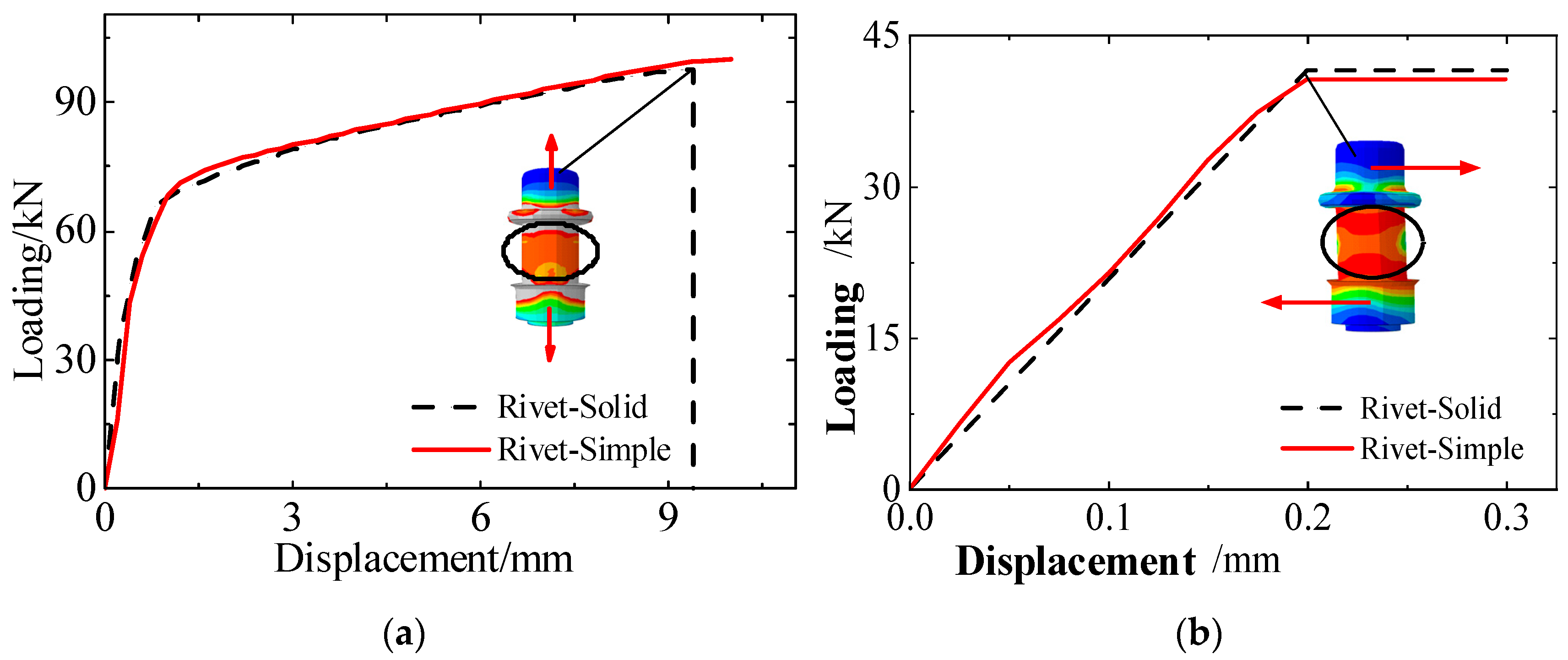
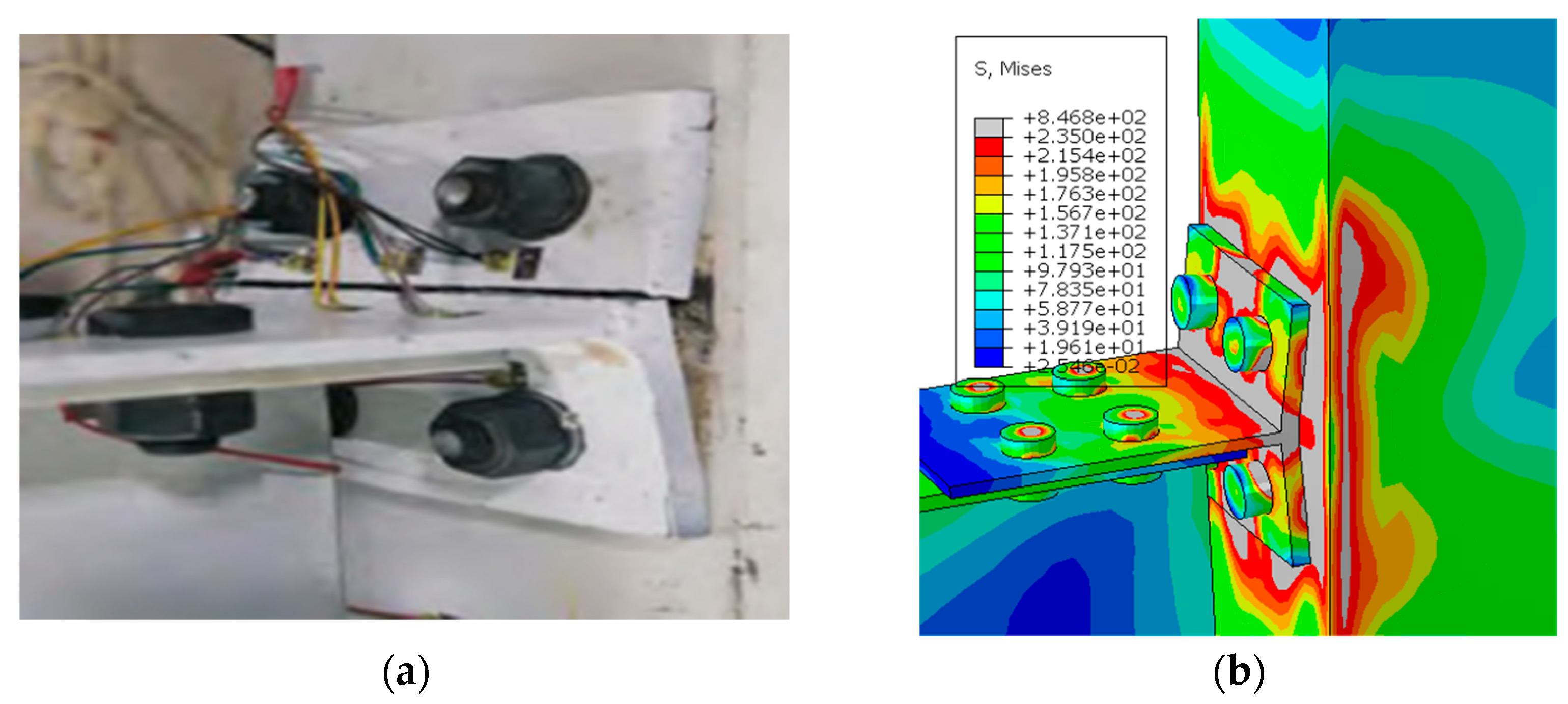
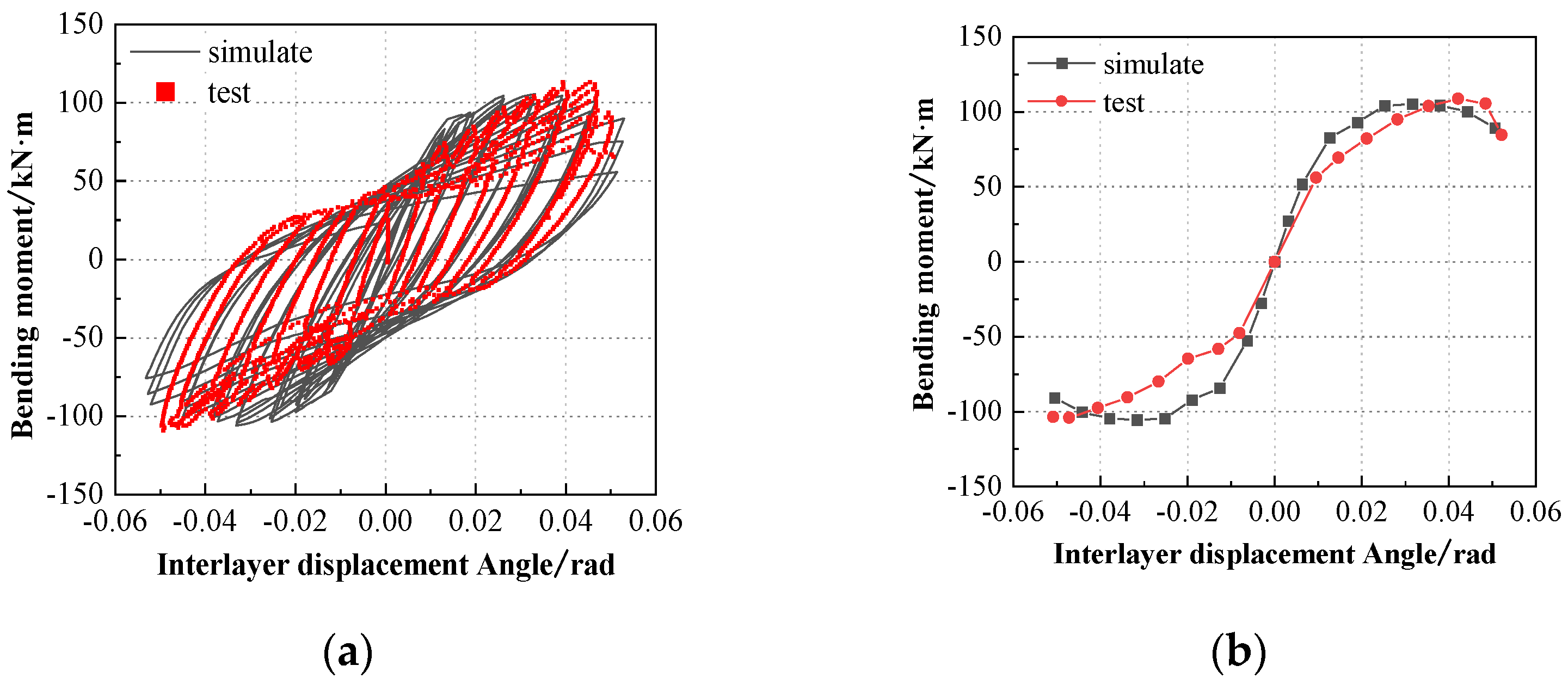
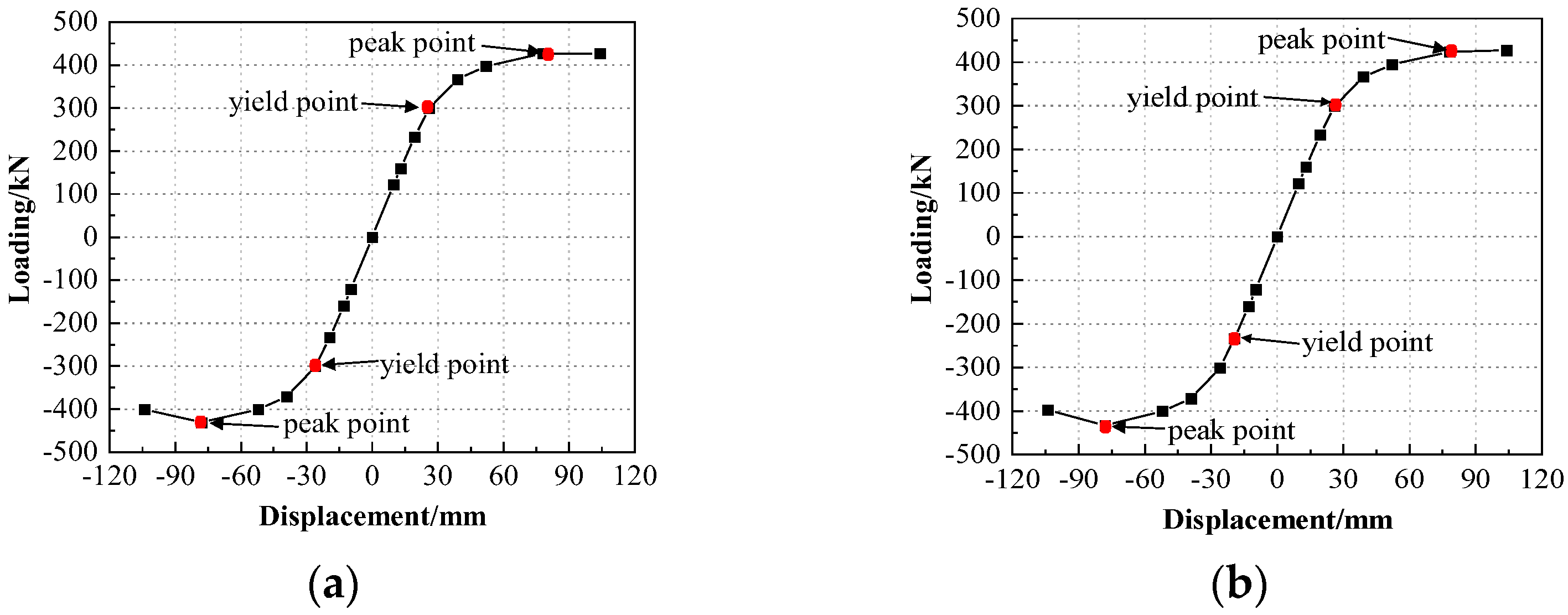
2.4. Model Verification
3. Seismic Performance Analysis
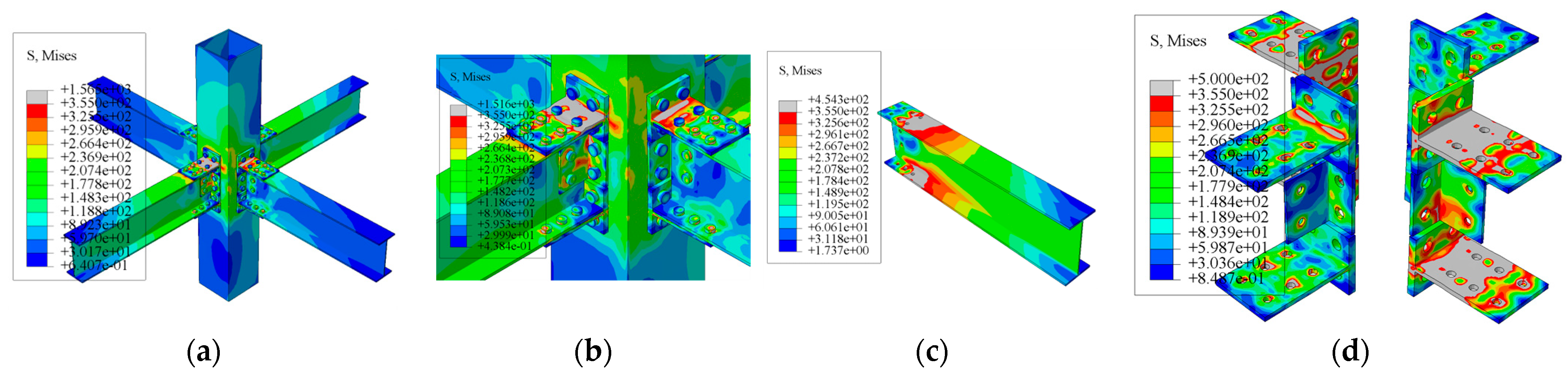
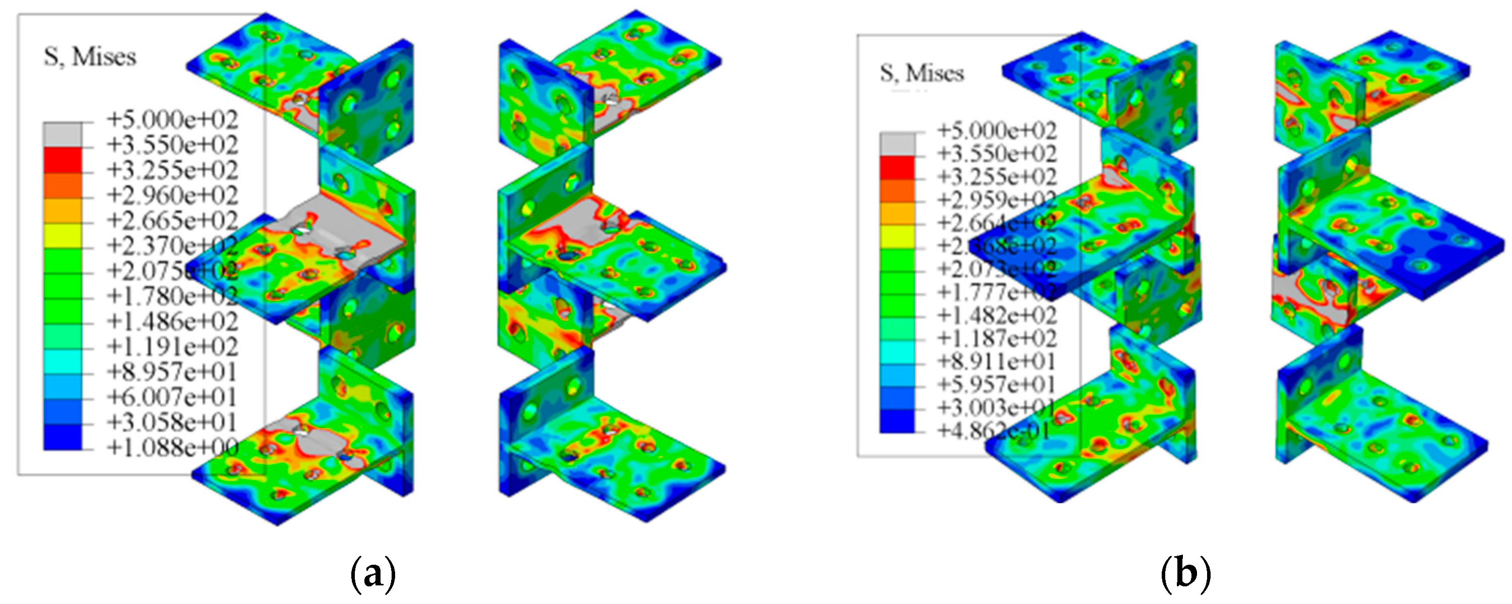
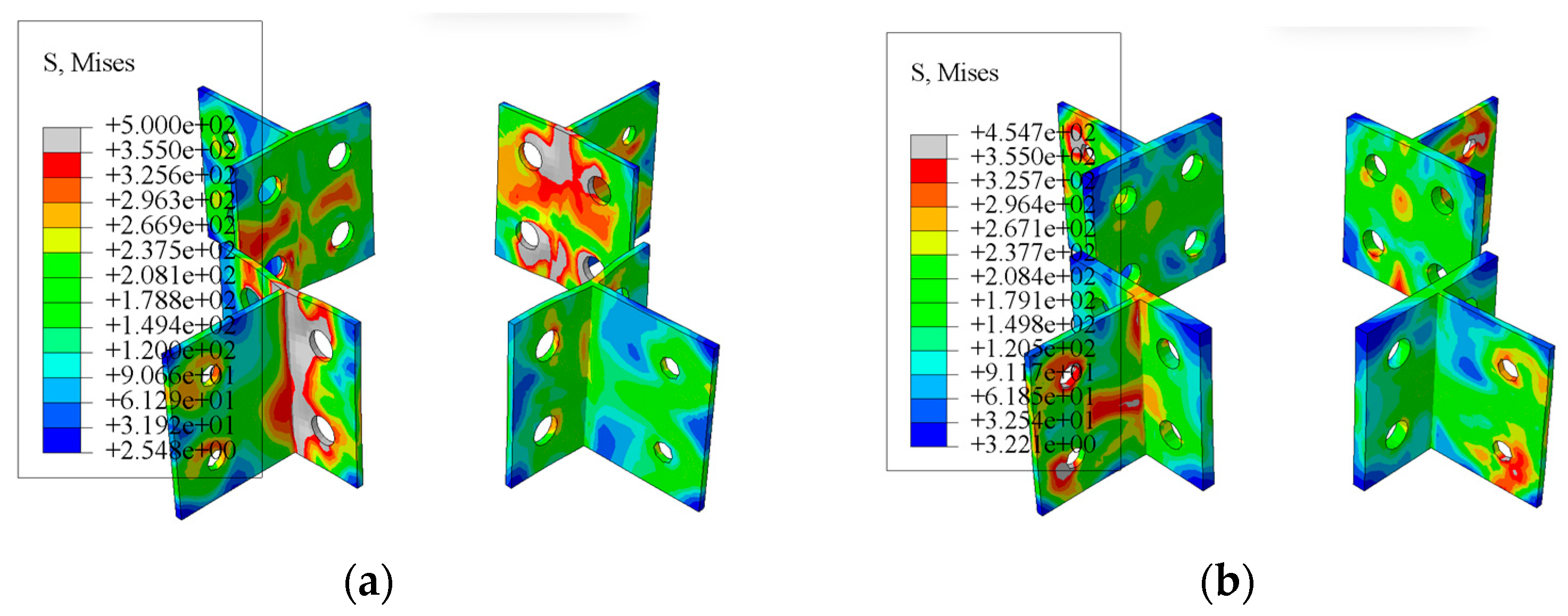
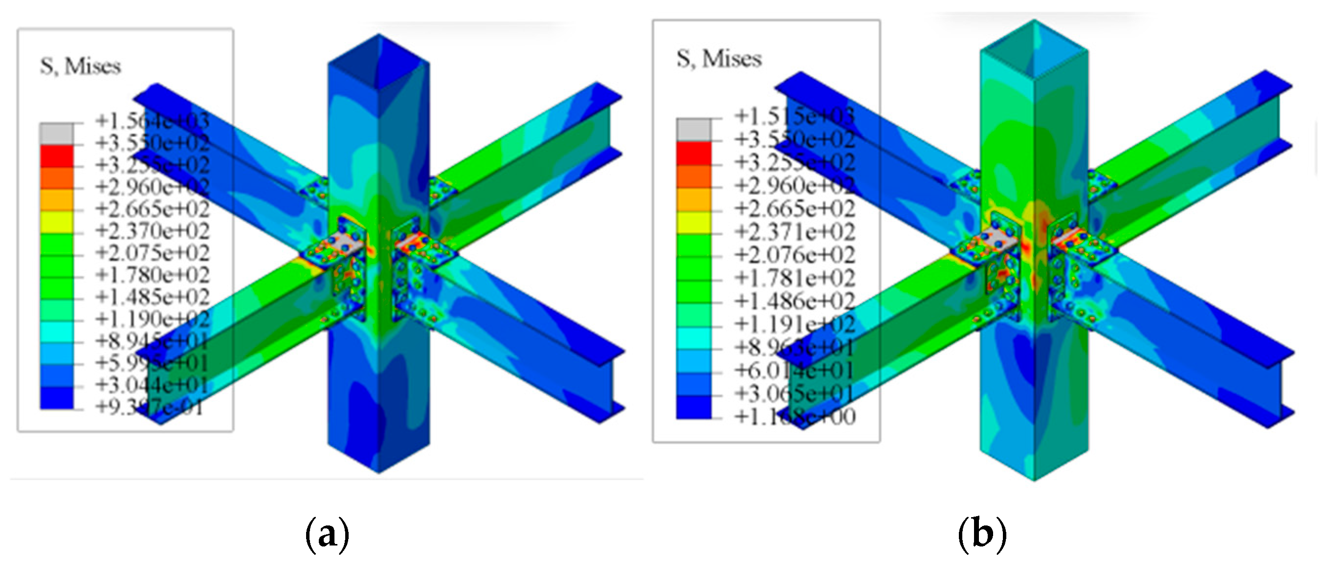
3.1. Failure Mode and Stress Development
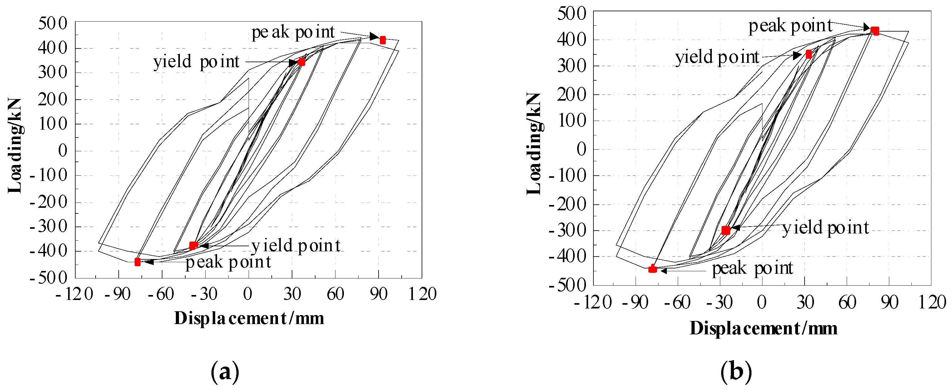
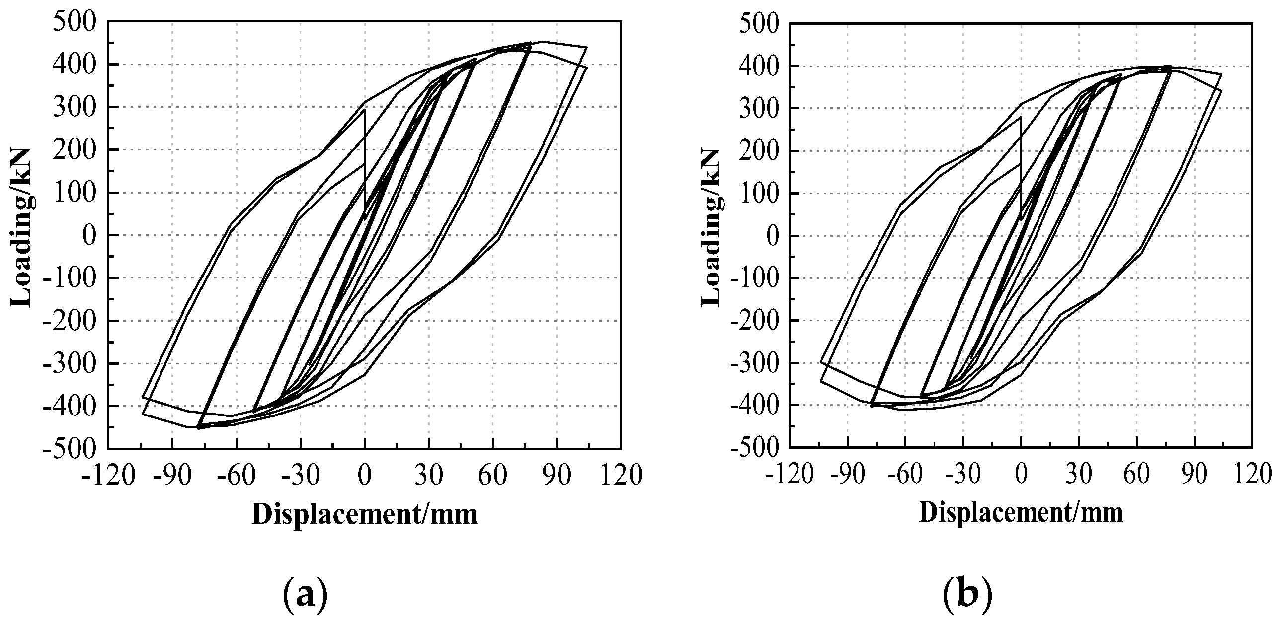
3.2. Hysteretic Curve and Skeleton Curve
4. Parametric Analysis
4.1. Parameter Analysis of T-Part 1
4.2. Parameter Analysis of T-Part 2
4.3. Parameter Analysis of Column Wall Thickness
4.4. Parameter Analysis of Axial Compression Ratio
4.5. Parameter Analysis of High-Strength Bolt Preload
5. Conclusions
- (1)
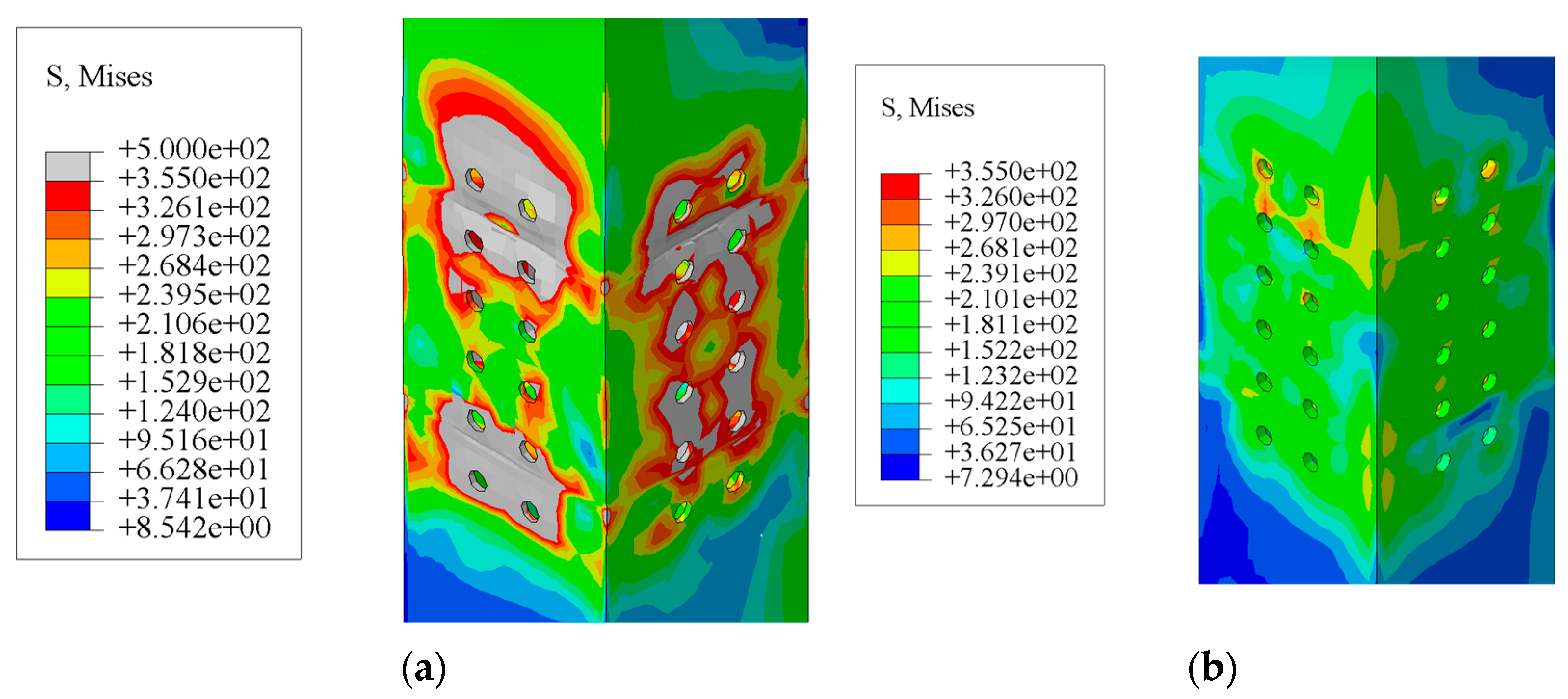
- For T-parts in unilateral bolted space joints, there are three failure modes: plastic-hinge failure of the beam flange; joint brittle failure caused by column wall-buckling failure; and joint brittle failure caused by T-part fracture. When the thickness of the column wall is extremely small, the bolt holes and their edges will yield due to stress concentration, and the column wall will buckle. Moreover, the buckling phenomenon becomes more pronounced as the displacement increases, eventually leading to the buckling failure of the column wall. When the web thickness of T-part 1 is thin, the first row of bolt holes on the web of T-part 1 is pulled off. To fully exploit the performance of the single-bolted space joints of T-parts, the stiffness of the joint domain can be enhanced by increasing the thickness of the web or column wall of the T-parts.
- (2)
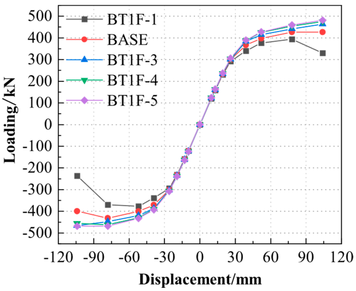
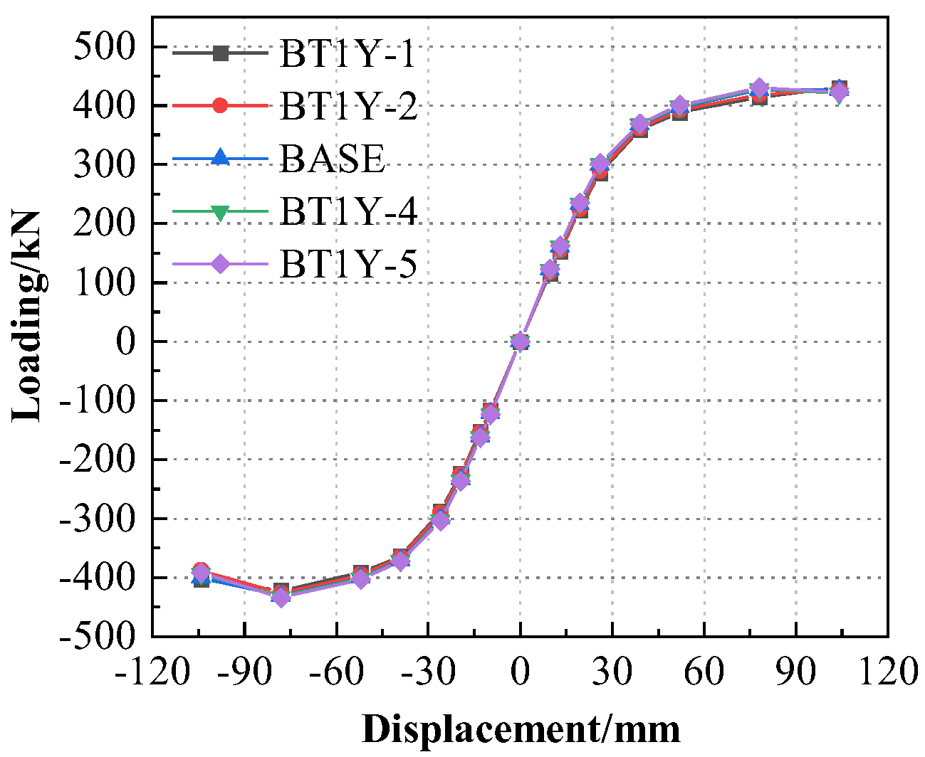
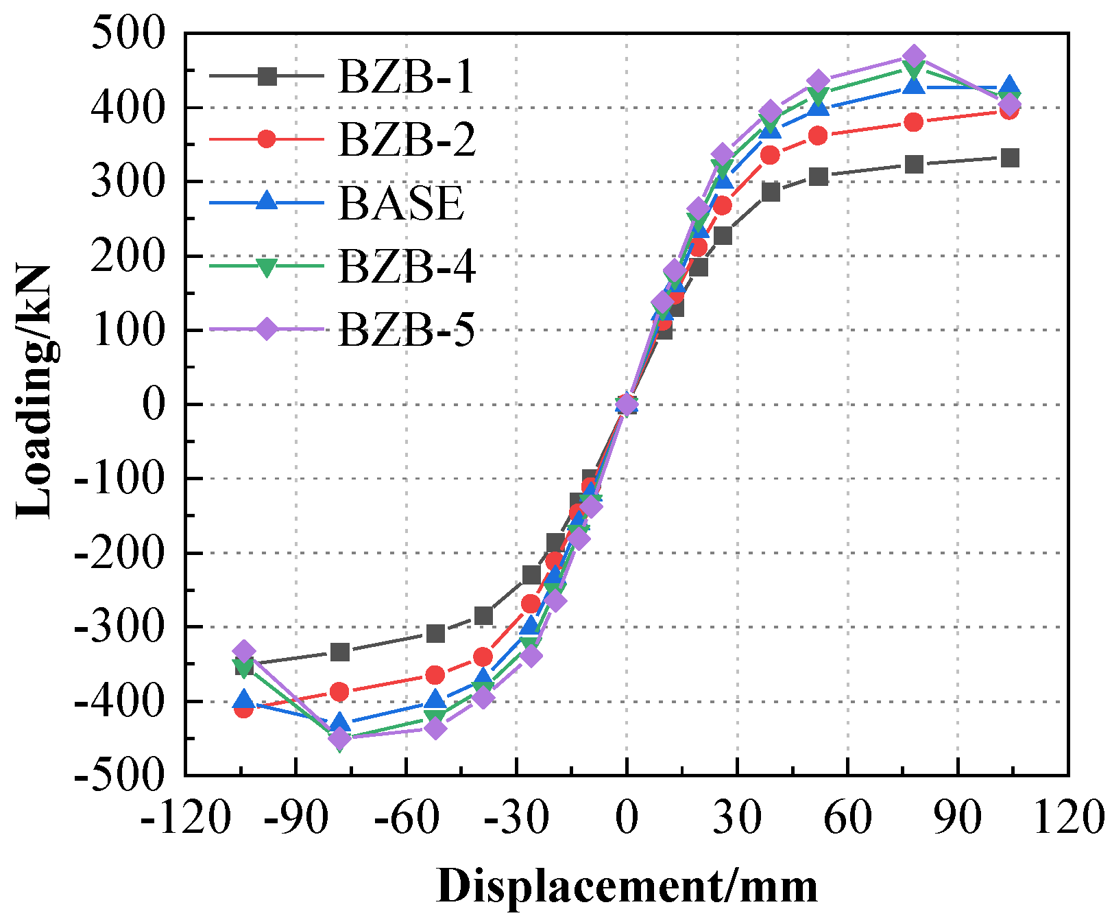
- The stiffness of T-part 1 exerts a significant influence on the joint. By increasing the thickness of the web plate of T-part 1, the bearing capacity and stiffness of the space joint can be enhanced. To prevent the brittle failure of joints resulting from the web fracture of T-part 1, achieve the ideal failure mode of forming a plastic hinge on the beam flange, and optimize the steel usage, it is recommended that the web thickness of T-part 1 should not be less than 18 mm. Specifically, compared with the BASE nodes, when the web thickness increases from 16 mm to 18 mm, the yield load and bearing capacity of the space node increase by approximately 12% and 16%, respectively, (see Figure 13).
- (3)
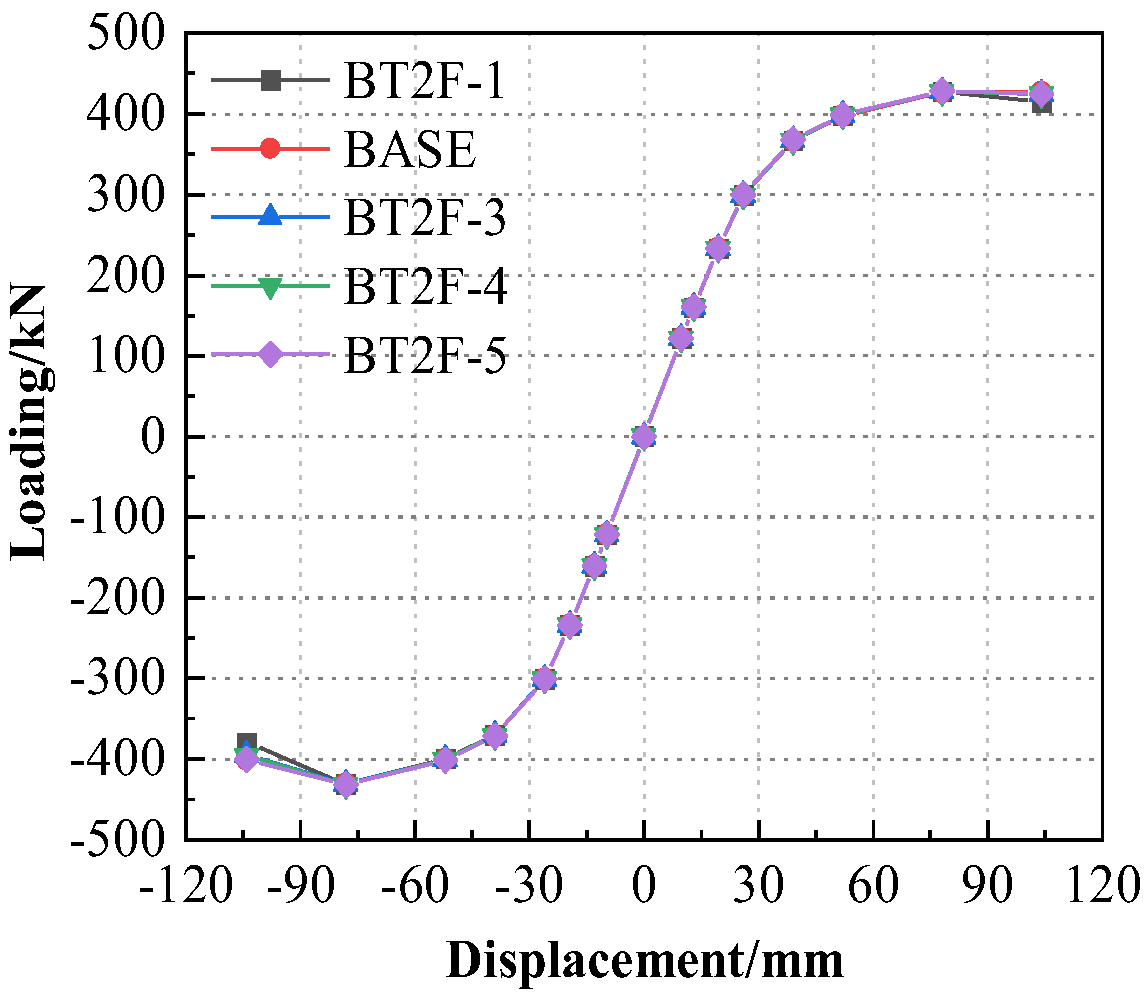
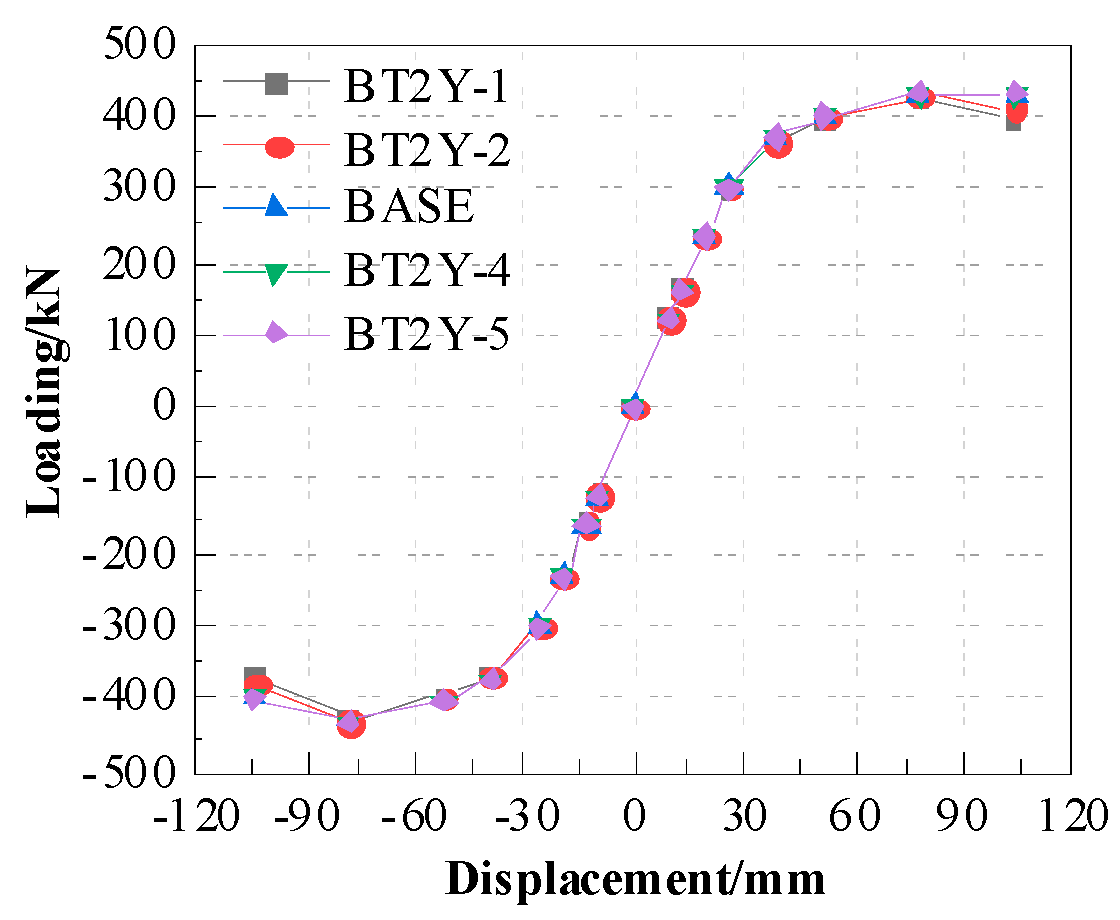
- The thickness variations in the web and flange of T-part 2 have a negligible impact on the seismic resistance of the joint. Whether the stiffness of T-part 2 decreases or increases, the yield load, bearing capacity, initial stiffness, and ductility of the joints do not exhibit significant changes. When the web thickness of T-part 2 increased from 6 mm to 14 mm, the yield load increased by only 0.8% (from 372.5 kN to 375.5 kN), and the peak load increased by 1.1% (from 435.2 kN to 439.9 kN) (Table 5, Figure 17). The stiffness varies by less than 6%, and the ductility coefficient (Δu/Δy = 2.7~2.8) is almost unchanged (Table 3).
- (4)
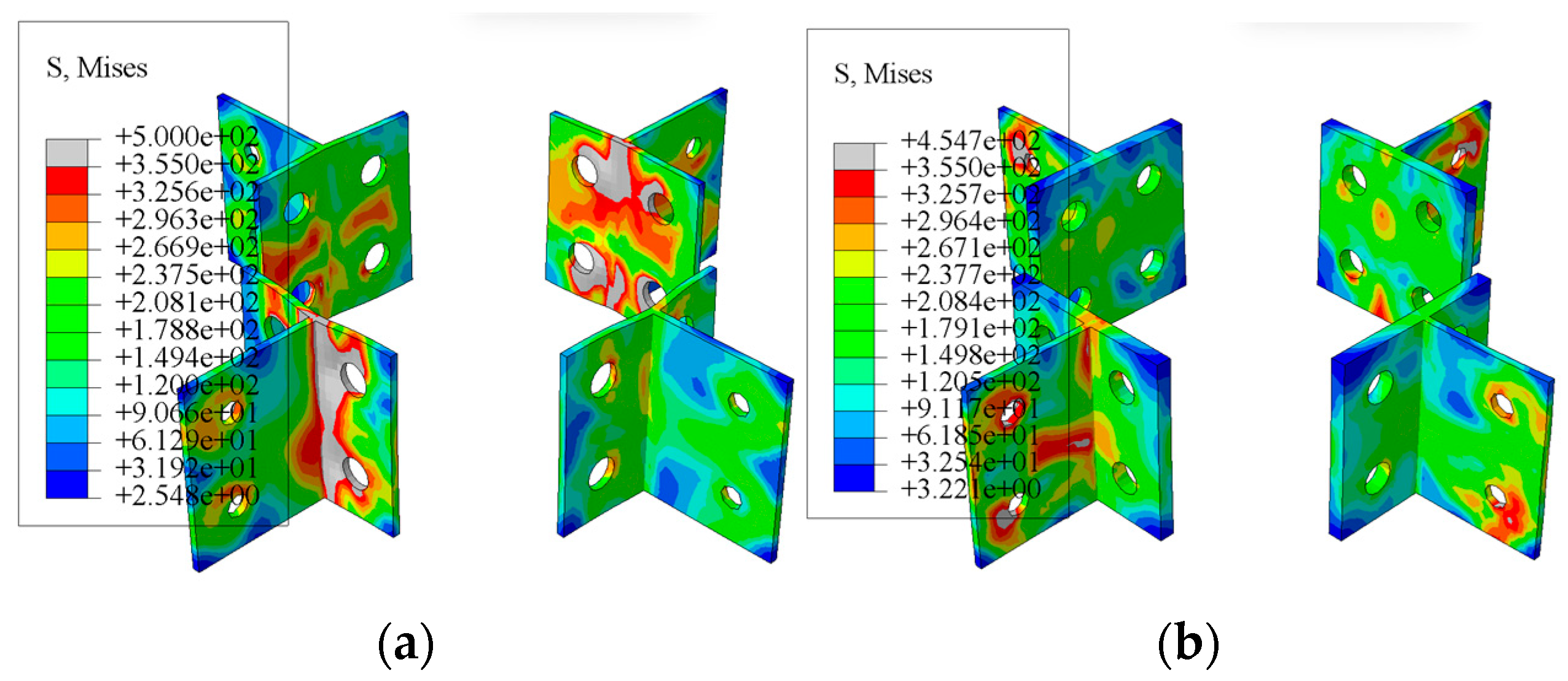
- When the thickness of the column wall is overly thin, the column wall is prone to buckling failure. As the wall thickness increases, the bearing capacity and stiffness of the joint increase. Additionally, the increase in wall thickness alleviates the deformation of the column wall to a certain degree. This paper recommends that the wall thickness of the joint column should be no less than the flange thickness of the steel beam and should not be less than 12 mm. When the column wall thickness increases from 10 mm to 12 mm, the yield load and bearing capacity increase by 37.85% and 33.4%, respectively, compared with the 10 mm thick column wall node (see Figure 20). When the column wall thickness increases (e.g., from 10 mm to 18 mm), the column wall stiffness increases significantly (initial stiffness increases by 38.12%), effectively limiting local buckling around the bolt hole (Figure 19b). The thicker column wall delays brittle failure (e.g., tearing) by preventing stress concentration, which in turn guides the plastic deformation to the H-shaped steel-beam flange, resulting in a plastic hinge at the beam end (Δu/Δy increased from 2.1 to 3.5).
- (5)
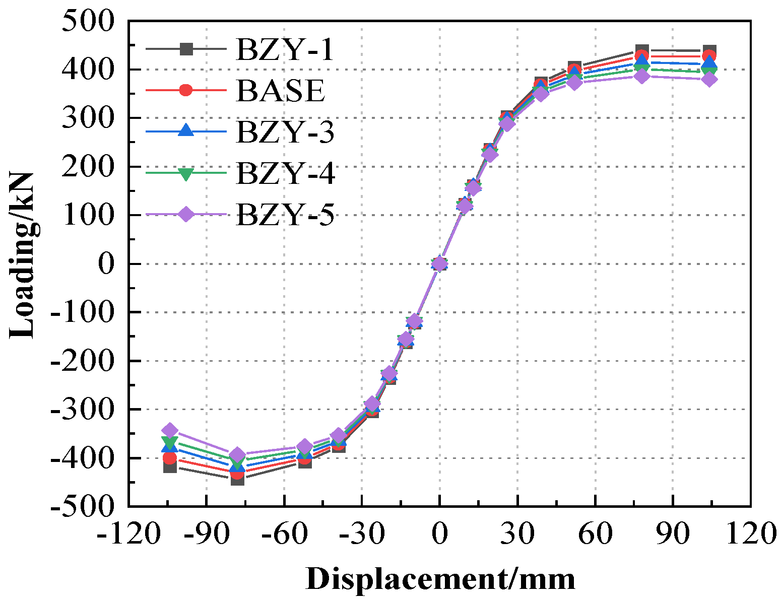
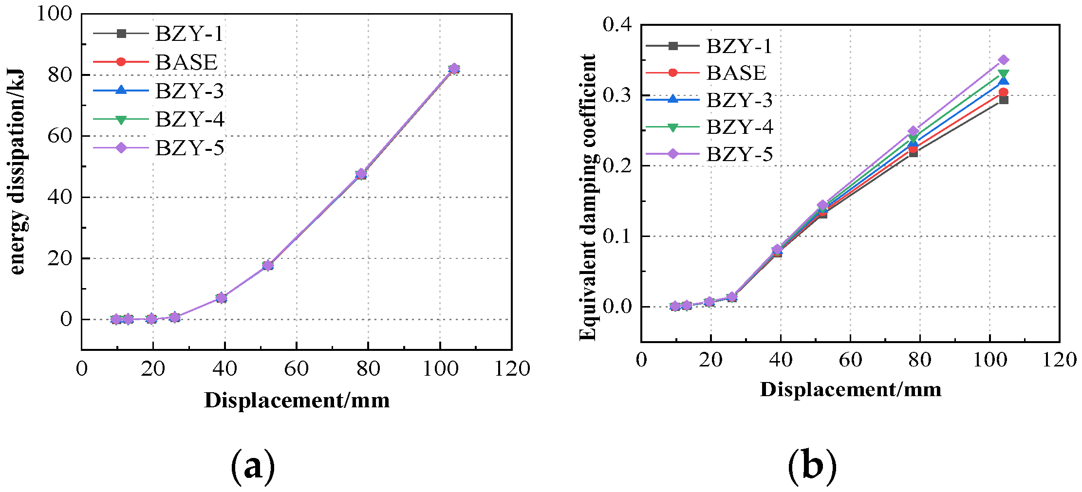
- As the axial compression ratio increases, the bearing capacity and stiffness of the joint decrease, yet the degree of stiffness reduction is not conspicuous. Conversely, the energy-dissipation capacity and ductility increase with the rise in the axial compression ratio.
- (6)
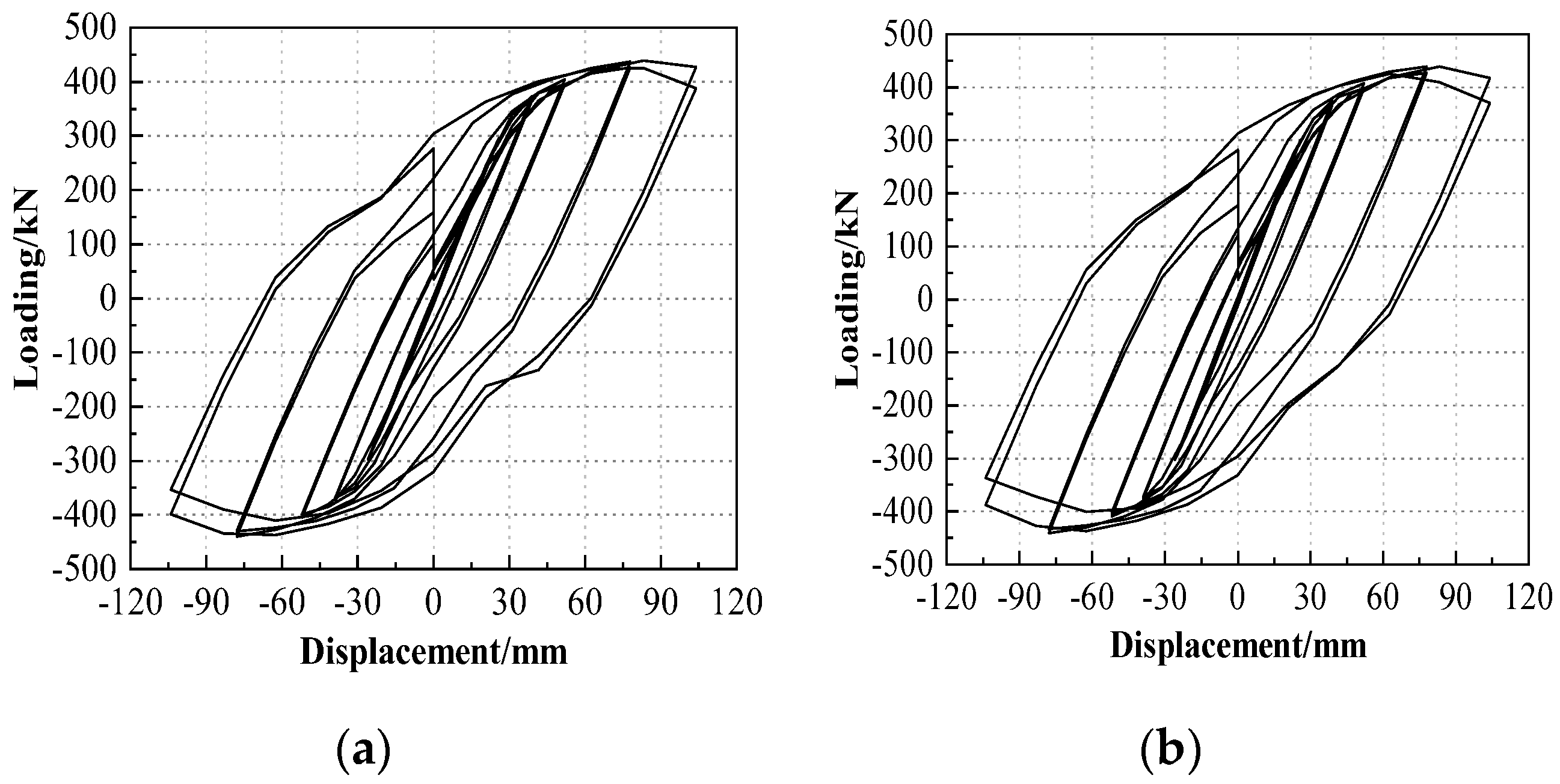
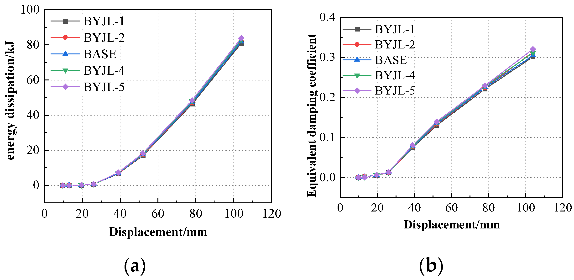
- The increase or decrease in the pre-tightening force of the high-strength bolt has no impact on the overall performance of the node. The yield load, bearing capacity, initial stiffness, and ductility of the joints with high-strength bolts do not change significantly as the preloading force varies. When the bolt preload increases from 180 kN to 270 kN, the yield load fluctuates ±1.9% (372.1 kN~379.5 kN), and the peak load fluctuates ±1.3% (436.8 kN~442.3 kN) (Table 3, Figure 28). These fluctuations are much lower than the material strength dispersion (Q355B steel yield strength standard deviation of about 5%).
- (7)
- Based on the research results, the recommended design threshold is given: The web thickness of the T-shaped part 1 is ≥18 mm (to ensure the formation of the plastic hinge, Δu/Δy ≥ 3.0); column wall thickness ≥ 12 mm (to prevent column wall buckling, initial stiffness ≥ 10 kN/mm); and axial compression ratio ≤ 0.4 (equilibrium bearing capacity and energy consumption, equivalent damping ≥ 0.25).
Author Contributions
Funding
Institutional Review Board Statement
Informed Consent Statement
Data Availability Statement
Conflicts of Interest
References
- Zhao, J.Y.; Wang, X.W.; Chu, H.B.; Sun, H.L.; Bu, X.; Liu, H.H. Experimental research on seismic performance of T-piece unilateral bolted beam-column joints. J. Xi’an Univ. Archit. Technol. (Nat. Sci. Ed.) 2022, 54, 665–674. [Google Scholar] [CrossRef]
- Erfani, S.; Asnafi, A.; Goudarzi, A. Connection of I-beam to box-column by a short stub beam. J. Constr. Steel Res. 2016, 127, 136–150. [Google Scholar] [CrossRef]
- Liu, X.C.; Chen, G.P.; Xu, L.; Yu, C.; Jiang, Z.Q. Seismic performance of blind-bolted joints for square steel tube columns under bending-shear. J. Constr. Steel Res. 2021, 176, 106395. [Google Scholar] [CrossRef]
- Bu, X.; Wang, X.W.; Gu, Q. Experimental study on seismic performance of spatial beam to side column connection with T-stub. J. Huazhong Univ. Sci. Technol. (Nat. Sci. Ed.) 2016, 44, 117–123. [Google Scholar] [CrossRef]
- Han, D.; Bu, X.; Wang, X.W.; Jiang, C. Experiment on seismic performance of spatial beam to corner column connection with T-stub. J. Zhejiang Univ. (Eng. Sci.) 2017, 51, 287–296. [Google Scholar] [CrossRef]
- Liu, C.W.; Wang, X.W.; Bu, X. Research on seismic behavior of steel frame beam to column connection with T-stub. Ind. Constr. 2018, 48, 162–168. [Google Scholar] [CrossRef]
- Lin, Y.; Wang, X.; Gong, J.; Wang, S.; Sun, H.; Liu, H. Seismic performance of an exterior joint between a square steel tube column and an H-shape steel beam. Sustainability 2023, 15, 3856. [Google Scholar] [CrossRef]
- Liu, Z.Y.; Tang, Q.S.; Dong, X.Y.; Weng, W.S.; Zhao, J.X.; Zhang, J.M. Experimental study on performance of the connection joints of cold-formed square steel tubular columns and H-shaped steel beams extension endplate using blind bolts. Build. Struct. 2021, 51, 57–63. [Google Scholar] [CrossRef]
- Liu, Z.Y.; Tang, Q.S.; Chen, W.; Zhong, M.; Li, B.Y.; Weng, W.S. Study on the performance of the blind bolted connection joints of the square steel tube column-H-shaped steel beam T-stub. Build. Struct. 2022, 51, 116–123. [Google Scholar] [CrossRef]
- Liu, Z.Y.; Tang, Q.S.; Chen, W.; Weng, W.S.; Hao, Y. Moment Resisting Behavior of Blind Bolted T-stub Connections Between Square Hollow Section Columns and H-shaped Beams. Prog. Steel Build. Struct. 2022, 24, 108–118. [Google Scholar] [CrossRef]
- Zhang, Y.F.; Wang, D.; Gao, J.Q.; Miao, Y.S.; Hu, H.T. Experimental study on hysteresis behaviors of T-stub joints with single-side bolt. Build. Struct. 2023, 53, 55–61. [Google Scholar] [CrossRef]
- Wang, W.; Li, M.; Chen, Y.; Jian, X. Cyclic behavior of endplate connections to tubular columns with novel slip-critical blind bolts. Eng. Struct. 2017, 148, 949–962. [Google Scholar] [CrossRef]
- Wang, W.; Li, L.; Chen, D. Progressive collapse behaviour of endplate connections to cold-formed tubular column with novel Slip-Critical Blind Bolts. Thin Walled Struct. 2018, 131, 404–416. [Google Scholar] [CrossRef]
- Wang, W.; Li, L.; Chen, D.; Xu, T. Progressive collapse behaviour of extended endplate connection to square hollow column via blind Hollo-Bolts. Thin Walled Struct. 2018, 131, 681–694. [Google Scholar] [CrossRef]
- American Institute of Steel Construction. Seismic Provisions for Structural Steel Buildings (No. 2). American Institute of Steel Construction. 2002. Available online: https://www.aisc.org/publications/steel-standards/aisc-341/ (accessed on 1 January 2025).
- ASCE/SEI 41-17; Seismic Evaluation and Retrofit of Existing Buildings. American Society of Civil Engineers/Structural Engineering Institute (ASCE): Reston, VA, USA, 2017.
- Jiang, L.; Li, H.; Chen, Y. Simplified modeling of bolted flange connections using spring-damping elements. Eng. Struct. 2020, 225, 111245. [Google Scholar] [CrossRef]
- Javelin-Tech. Finite Element Modeling Guidelines for Mechanical Fasteners (Technical Report). 2024. Available online: https://www.javelin-tech.com/blog/tag/solidworks-2024/ (accessed on 1 January 2025).
- Zheng, Y.; Wang, X.; Bu, X. Cyclic behavior of simplified UHPC beam-column joints: Experiment and modeling. J. Constr. Steel Res. 2019, 155, 175–188. [Google Scholar] [CrossRef]
- Dassault Systèmes. ABAQUS Analysis User’s Manual, Version 2023; Dassault Systèmes: Singapore, 2022. [Google Scholar]
- Ding, F.X.; Wei, X.Y.; Pan, Z.C.; Wang, L.P.; Lei, J.X.; Chen, J.; Hu, M.W.; Yang, J. Experimental study on seismic behavior of square CFST column-composite beam single-side bolted rigid joint under high axial compression. J. Build. Struct. 2023, 44, 105–115. [Google Scholar] [CrossRef]
- Bu, X.; Gu, Q.; Wang, X.W. Experimental study on the seismic performance of three-dimensional beam to middle column connection with T-stub. Eng. Mech. 2017, 34, 105–116. [Google Scholar] [CrossRef]


| Type | Specification (mm) | Quantity |
|---|---|---|
| Square-steel column | 400 × 400 × 14 | 1 |
| H-shaped steel beam | HN400 × 200 × 8 × 13 | 4 |
| T-part 1 | T320 × 200 × 16 × 24 | 8 |
| T-part 2 | T180 × 200 × 8 × 12 | 4 |
| M24 high-strength bolt | Φ24 | 56 |
| M24 single-side bolt | Φ24 | 48 |
| Type | Solid Model | Cell Type | Meshing Technique |
|---|---|---|---|
| Square-steel column |  | Type of four-node reduced integration unit: S4R | Free technology Advanced algorithm |
| H-shaped steel beam | 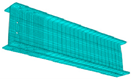 | Type of four-node reduced integration unit: S4R | Free technology Advanced algorithm |
| T-part 1 | 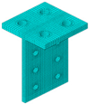 | Type of eight-node reduced integration unit: C3D8R | Free technology Advanced algorithm |
| T-part 2 |  | Type of eight-node reduced integration unit: C3D8R | Free technology Advanced algorithm |
| High-strength bolt |  | Type of eight-node reduced integration unit: C3D8R | Structural technique |
| Loading Direction | Yield Point | Peak Point | Limiting Point | Ductility Coefficient | Error | |||
|---|---|---|---|---|---|---|---|---|
| Py (kN) | Δy (mm) | Pmax (kN) | Δmax (mm) | Pu (kN) | Δu (mm) | |||
| X+ | 374.04 | 41.95 | 439.36 | 83.20 | 426.45 | 104 | 2.48 | 8.2%/7.5% |
| X− | 378.37 | 42.22 | 440.55 | 78 | 400.10 | 104 | 2.46 | 7.9%/6.8% |
| Z+ | 373.26 | 42.22 | 438.05 | 78 | 426.74 | 104 | 2.46 | 9.1%/8.1% |
| Z− | 379.42 | 42.46 | 442.27 | −78 | 397.55 | 104 | 2.45 | 6.5%/5.9% |
| Abbreviation | Implication |
|---|---|
| SCBB | Square steel tube column-bolted beam |
| BT1F | Different web thicknesses T-part 1 |
| BT1Y | Different flange thicknesses T-part 1 |
| BT2F | Different web thicknesses T-part 2 |
| BT2Y | Different flange thicknesses T-part 2 |
| BZB | Base joint with bolted connection |
| BZY | Bolted joint with different axial load ratios |
| JD-FSH | Joint with different flange thickness of steel H-section |
| JD-YJL | Joint with different web thickness of Y-shaped steel |
| BYJL | Bolted joint with different yield preload levels |
| Model number | BT1F-1 | BT1F-2 | BT1F-3 | BT1F-4 | BT1F-5 |
| Web thickness (mm) | 13 | 15 | 17 | 19 | 21 |
| Model number | BT1Y-1 | BT1Y-2 | BASE | BT1Y-4 | BT1Y-5 |
| Flange thickness (mm) | 20 | 22 | 24 | 26 | 28 |
| Model number | BT2F-1 | BASE | BT2F-3 | BT2F-4 | BT2F-5 |
| Web thickness (mm) | 6 | 8 | 10 | 12 | 14 |
| Model number | BT2Y-1 | BT2Y-2 | BASE | BT2Y-4 | BT2Y-5 |
| Flange thickness (mm) | 8 | 10 | 12 | 14 | 16 |
Disclaimer/Publisher’s Note: The statements, opinions and data contained in all publications are solely those of the individual author(s) and contributor(s) and not of MDPI and/or the editor(s). MDPI and/or the editor(s) disclaim responsibility for any injury to people or property resulting from any ideas, methods, instructions or products referred to in the content. |
© 2025 by the authors. Licensee MDPI, Basel, Switzerland. This article is an open access article distributed under the terms and conditions of the Creative Commons Attribution (CC BY) license (https://creativecommons.org/licenses/by/4.0/).
Share and Cite
Ju, H.; Jiang, W.; Hu, X.; Zhang, K.; Guo, Y.; Yang, J.; Hao, K. A Study on the Seismic Performance of Steel H-Column and T-Beam-Bolted Joints. Appl. Sci. 2025, 15, 4643. https://doi.org/10.3390/app15094643
Ju H, Jiang W, Hu X, Zhang K, Guo Y, Yang J, Hao K. A Study on the Seismic Performance of Steel H-Column and T-Beam-Bolted Joints. Applied Sciences. 2025; 15(9):4643. https://doi.org/10.3390/app15094643
Chicago/Turabian StyleJu, Hongtao, Wen Jiang, Xuegang Hu, Kai Zhang, Yan Guo, Junfen Yang, and Kaili Hao. 2025. "A Study on the Seismic Performance of Steel H-Column and T-Beam-Bolted Joints" Applied Sciences 15, no. 9: 4643. https://doi.org/10.3390/app15094643
APA StyleJu, H., Jiang, W., Hu, X., Zhang, K., Guo, Y., Yang, J., & Hao, K. (2025). A Study on the Seismic Performance of Steel H-Column and T-Beam-Bolted Joints. Applied Sciences, 15(9), 4643. https://doi.org/10.3390/app15094643