Using Bi-Temporal Lidar to Evaluate Canopy Structure and Ecotone Influence on Landsat Vegetation Index Trends Within a Boreal Wetland Complex

Abstract

Wetland ecosystems are sensitive to climate variation, yet tracking vegetation type and structure changes through time remains a challenge. This study examines how Landsat-derived vegetation indices (NDVI and EVI) correspond with lidar-derived canopy height model (CHM) changes from 2000 to 2018 across the wetland landscape of the Peace–Athabasca Delta (PAD), Canada. By comparing CHM change and NDVI and EVI trends across woody and herbaceous land covers, this study fills a gap in understanding long-term vegetation responses in northern wetlands. Findings show that ~35% of the study area experienced canopy growth, while 2% saw a reduction in height. CHM change revealed 11% ecotonal expansion, where shrub and treed swamps encroached on meadow and marsh areas. NDVI and EVI correlated significantly (p < 0.001) with CHM, particularly in shrub swamps (r² = 0.40, 0.35) and upland forests (NDVI r² = 0.37). However, EVI trends aligned more strongly with canopy expansion, while NDVI captured mature tree height growth and wetland drying, indicated by rising land surface temperatures (LST). These results highlight the contrasting responses of NDVI and EVI—NDVI being more sensitive to moisture-related changes such as wetland drying, and EVI aligning more closely with canopy structural changes—emphasizing the value of combining lidar and satellite indices to monitor wetland ecosystems in a warming climate.

1. Introduction

In northern deltaic minerotrophic wetland ecosystems, ecotones represent important hydro-ecological transition zones where vegetation height and cover vary from open water to marsh to wet meadow and/or water-tolerant shrub species along local elevation gradients [1,2,3,4]. Local upland areas (e.g., levees) that surround river channels have deeper aerated soils where less water-tolerant conifer (e.g., Picea mariana, Larix laricina, etc.) and deciduous (Acer spp., Populus tremuloides Michx., etc.) trees establish taller canopy woodland ecosystems [5,6,7,8,9,10]. Local terrain and groundwater gradients are a determining factor in establishing the spatial patterns of vegetation type, cover and height zonation across such environments, with seasonal and long-term variations influenced by hydro-climatic conditions [8,9]. Aquatic-, herbaceous-, and shrub-dominated ecotones at the margins of wetlands are also susceptible to interannual climate variability and therefore also alter their extent relative to local limiting [11]. Meanwhile, the slower growth associated with dryland forest ecosystems means that changes in woodland ecotones tend to be associated either with episodic mortality events (ecotone contraction or forest cover loss, e.g., Carpino et al. [12] and Birch et al. [13]) or longer-term successional growth processes (ecotone expansion, e.g., Tremblay et al. [14], Frost and Epstein [15], Jackson et al. [16]).

Quantification of ecotone change requires long-term monitoring. However, field data necessary for understanding the characteristics of northern ecosystem changes [17] have largely been limited due to the broad spatial extent and high deployment costs associated with these remote and in many instances inaccessible northern wetlands [18]. To address these issues, remote sensing approaches, particularly through the multi-decade Landsat program, have become necessary for studying trends in vegetation indices (VIs) as they prove consistent coverage multiple times per year over large areas.

Two indices, the Normalized Difference Vegetation Index (NDVI) [19] and the Enhanced Vegetation Index (EVI) [20,21] have been used to quantify trends in northern ecosystem change [22,23,24,25]. Higher positive VI values are typically interpreted as healthier or denser vegetation cover [26,27], thus providing a means to track wetland ecotone structure or extent change trajectories. NDVI, an indicator of photosynthetic activity [19], has been widely applied in northern, low-biomass environments impacted by climate change [28,29], though it is also influenced by factors such as soil exposure, topography and atmospheric conditions, which can alter, offset or mask the vegetation signal [30,31]. NDVI tends to saturate in dense or multi-layered vegetated canopies with a leaf area index (LAI) greater than 3 [32,33], and its performance varies by land cover and growth stage [31]. EVI is widely used instead of NDVI in many scenarios due to its reduced potential for saturation and adjustment for non-linear soil influences on pixel spectral characteristics and the inclusion of a blue band to counteract the effects of the atmosphere [34,35]. These make the index particularly resilient in areas with high soil visibility or dense canopy cover [34], though it remains sensitive to the same geometric and surface reflection variations that influence NDVI [36].

Characterization and quantification of how VI values relate to properties of vegetation height and cover, and over time, and how VI trends relate to canopy growth, ecotone expansion or dieback within boreal wetland complexes have not been systematically examined. Understanding these VIs and their relationship with vegetation height and cover (indicators of productivity) for a range of wetland and adjacent landcover classes is important as this will aid in the interpretation of NDVI and EVI trends across deltaic wetland environments and other similar northern landscapes, where global landcovers are undergoing dramatic rates of change [37,38].

To explore the influence of changing ground surface moisture conditions on observed VI changes, Land Surface Temperature (LST) trends have been used as a proxy for changing soil saturation (comparatively cool) or dryness (comparatively warm) [39,40,41,42,43,44,45]. While radar-based remote sensing techniques are capable of estimating soil moisture [46], their applicability is often limited by inconsistent spatial and temporal coverage, particularly in large-scale or long-term studies [47].

The over-arching goal of this study is to identify any landcovers and associated ecotonal changes where canopy characteristics and VI patterns systematically converge or diverge in space or through time over a remote and dynamic northern wetland complex: the Peace–Athabasca Delta (PAD), found in north-eastern Alberta, Canada. To address the need for spatially extensive field observations of vegetation structure, bi-temporal lidar-derived canopy height, cover and change (2000 and 2016/2018) were compared to Landsat-derived NDVI and EVI trends across a range of wetland landcover classes. The availability of lidar measurements provides three-dimensional canopy structure and elevation of the landscape including canopy height [48,49], wetland and riparian environments [48,50,51] and if temporal data exist, change in these structures over time [9,50,51,52,53,54,55,56]. Understanding vegetation responses to hydroclimatic change in the PAD provides insight applicable to similar wetland ecosystems globally, many of which are undergoing rapid ecological transitions [57,58,59,60].

More specifically, this study will address three objectives:

1.

To evaluate the hypothesis that Landsat-derived VIs are correlated with spatio-temporally coincident lidar-derived Canopy Height Models (CHMs) for at least some landcovers—specifically woody wetlands (e.g., shrub swamp, treed swamps) and upland forest areas—where VI values are expected to better reflect vertical vegetation structure, given that VIs are proxies for green leafy foliage cover and biomass tends to increase with mean canopy height [61]. This is evaluated through two sub-hypotheses:

(a)

Based on the assumption that EVI is more sensitive to variations in canopy structure and density, and typically yields higher values in areas of taller canopy [62], the first sub-hypothesis tests for a stronger positive correlation between CHM and EVI than for NDVI;

(b)

Given that foliage cover and vegetation height are not the same quantity, the second sub-hypothesis tests for significant differences in the relationships between CHM and VI (and their changes/trends) across distinct landcover classes [63].

2.

To examine how trends in NDVI and EVI correspond with changes in canopy height over time and characterize spatial correspondences between regions of contiguous ecosystem or landcover expansion (or shrinkage) and regions of VI trend increase (or decrease). It is not expected that NDVI or EVI increasing (greening) or decreasing (browning) trends will consistently or strongly correlate with increases or decreases in lidar-derived CHM magnitudes at the grid cell level. Specifically, it is expected that any spatial correspondence between aggregate regions of VI trend- and CHM-based change will be most apparent where ecosystem height growth and foliage infilling are most pronounced, i.e., those associated with woody (shrub or tree) ecotonal expansion.

3.

To explore differences in the EVI and NDVI trend response to changing wetland conditions that are associated with long term changes in soil surface saturation inferred from trends in LST, particularly in non-woody wetland types.

2. Materials and Methods

2.1. Study Area

The Peace–Athabasca Delta (PAD), located near 58.5° N and 112.0° W (Figure 1a,b), lies within Wood Buffalo National Park in northwestern Canada. While the Park is recognized as a UNESCO World Heritage site, the PAD itself is a Ramsar designated wetland site of global significance [64]. Local relief ranges from ~209 to 220 m asl, with limited ground-level visibility due to dense willow shrubs and trees [8]. Lakes and wetlands receive water from precipitation and overbank flooding, with evapotranspiration as the primary loss mechanism [65,66]. Since the mid-1970s, rising mean annual temperatures and slightly reduced precipitation have led to increased wildfire frequency, reduced open water and marsh areas, and expansion of woody vegetation—signs of overall landscape drying [67].

The area of interest in this study was limited to regions where bi-temporal lidar coverages were available (175 km²—including open water and all other landcovers), from the years 2000 and 2016/2018 (Figure 1b). According to Ducks Unlimited Canada [68] landcover classification, the majority of the surveyed areas comprised shrub and hardwood swamps, emergent and meadow marshes and upland conifer and deciduous (Figure 1c,d). Swamps in this area are mineral wetlands, featuring fluctuating water tables and seasonal flooding [8]. The most common type of swamp class is shrub swamp, and these are prevalent in successional and meadow areas of the PAD, where groundwater levels fluctuate [8,68]. Extensive areas of marsh were situated around large lakes and flooded river valleys. The vegetation in marshes primarily includes emergent species: cattail (Typhaceae), bulrush (Scirpus), horsetail (Equisetum fluviatile), and wet graminoids including bluejoint (Calamagrostis canadensis). Drier woody upland areas of the PAD typically consist of a combination of white spruce (Picea glauca) and black spruce (Picea mariana) conifers, as well as some deciduous species, which are dominated by aspen (Populus tremuloides) [8,68]. A detailed breakdown of landcover classes and their areas is provided in Section 2.2.1.

2.2. Data Sources

2.2.1. Land Cover Data

The Wood Buffalo National Park Enhanced Wetland Classification (EWC) [68] circa 2017/2018 used in this study has a reported overall accuracy of ~75%. Dominant landcovers exceeding 3% of total area across the four lidar surveyed polygons were examined. Given that the current study explicitly examined open water variations through time, the static open water landcover class (including mudflat/salt flats and aquatic bed) was ignored (18.1 km² in total). The dominant classes included in the analysis are: (i) marsh (26.7% of the study area), (ii) shrub swamp (36.5%), (iii) treed swamp (11.2%), and (iv) upland forest (12.3%). Here, the “marsh” class was an amalgamation of ‘emergent’ and ‘meadow’ marsh classes, as these are temporally variable and interchangeable due to subtle variations in water level and, therefore, cannot be assumed to be static throughout the period of analysis or even a single year. All upland vegetation (Figure 1) was considered one class, “upland forest”. However, two swamp classes were maintained, “shrub swamp” and all other swamp classes (Figure 1) as “treed swamp”.

2.2.2. Landsat Imagery

Landsat Collection 2 Level 2 [69,70,71,72,73,74,75] atmospherically corrected Surface Reflectance image products (2000 to 2018) were accessed via Google Earth Engine for VI generation. Scan line corrector (SLC)-off issues associated with ETM+ data were mitigated by constraining all images for a given year’s composite to a single sensor, i.e., all available Collection 2 Landsat 7 imagery from 2000 to 2002, Landsat 5 from 2004 to 2011 and Landsat 8 from 2013 to 2018 (no cloud free data available in 2003 or 2012). Summer imagery (1 June to 31 August) were used to minimize the effect of vegetation phenology on VIs.

2.2.3. Airborne Lidar and Photography

Lidar data were collected using a dual-return Optech Inc. ALTM 1225 sensor (Optech Inc., Vaughan, ON, Canada) on 17 June 2000 [76] and a multi-return multi-channel Teledyne Optech Titan sensor on 4 August 2016 and 24 July 2018 (summer growing season), each operating at approximately 1000 m above ground. The pulse repetition frequencies were 25 kHz for the ALTM and 75 kHz per channel for the Titan, with fixed scan angles of 20° and 24–25°, respectively. The surveyed transects achieved returned point densities ranging from 0.6 to 6.8 returns per square meter. Variations in data acquisition parameters and point density outputs across the lidar datasets are due to the advances in technology over the last two decades [77].

Given sensor settings and survey configuration can impact laser pulse interactions with vegetation and, therefore, the distribution of returns within vegetation canopies [78], only upper canopy surfaces were compared over time using first and single returns. As explained in Section 2.3.2, lidar-derived CHM were generated at a 5 m grid cell resolution, which was less than the lowest point density dataset to mitigate density variations in the data (e.g., Lim et al. [79]). Figure 1b shows the spatial coverage of the lidar campaigns of 2000, 2016 and 2018 (A, B, C and D).

2.3. Analysis

2.3.1. Landsat Time Series

The methodological workflow is summarized in Figure 2. Processing began by applying scaling factors to convert pixel values to reflectance, ensuring consistency across imaging sessions and sensors [75]. Saturated pixels were then identified and removed [80,81], followed by masking and removing clouds and cloud shadows using the Quality Assessment bands [81]. Landsat imagery was then reprojected to match the lidar coordinate system (NAD83 CSRS, UTM Zone 12 North) for spatial alignment.

To mitigate cloud and shadow influences within the Landsat image time series, median image compositing was applied to create annual summertime composites [82,83,84,85]. To remove the short-term influence of lowering or increasing water levels (i.e., drying and/or flooding) from the VI trend analyses, all open water lakes and channels were masked out of the study polygons (e.g., Ju and Masek [86]) using Modified Normalized Difference Water Index (MNDWI), which is the ratio of the (green—SWIR) and (green + SWIR) [87]. Based on visual assessments, pixel MNDWI values > 0.1 were selected to define a binary water mask, and all such areas were excluded from further analysis.

NDVI and EVI were used as proxies for vegetation greenness and canopy structure. NDVI, calculated as (NIR − Red)/(NIR + Red), is sensitive to chlorophyll content [19], while EVI = 2.5 × (NIR − Red)/(NIR + 6 × Red − 7.5 × Blue + 1) adjusts for atmospheric and background effects using the blue band, improving performance in dense vegetation [20,21]. NDVI and EVI were created for each annual composite in Google Earth Engine [88]. VI trends were assessed using Theil–Sen median trend analysis [89,90], a robust non-parametric method that is minimally affected by outliers [91,92,93,94,95]. The procedure calculates the slope of the line connecting medians for each pair of points in the dataset [93,96]. The direction of the Theil–Sen slope indicates vegetation changes where positive when “greening” (increase in vegetation) and negative when signifying “browning” (decline in vegetation), and it can be interpreted as the rate of change trend over time [90]. Only Theil–Sen slopes with p-values below 0.05 and Z-scores exceeding 1.96 were considered significant, ensuring a minimum 95% confidence level [93,97,98] (Figure 2).

Summertime LST (°C) was obtained from Landsat thermal bands (Band 6 for Landsat 5 and 7, and Band 10 for Landsat 8) [99,100], and Theil–Sen slopes of the LST time series were extracted for all land pixels. These trends were assumed to be proxies for changing proportions of sensible and latent heat exchange following change in soil surface saturation or the underlying shallow groundwater table, as areas of nearby open water fluctuate [101,102]. In general, an increasing LST trend is assumed to show a drying soil surface as more of the available energy goes into sensible heating of the ground surface instead of the latent heat of water evaporation.

2.3.2. Lidar-Derived Canopy Structure

To ensure alignment of bi-temporal lidar data, point cloud elevations for the 2000 dataset were block-adjusted to the corresponding 2016 and 2018 datasets by comparing point clouds over unchanging open terrain features. This corrected minor elevation biases (0.3–0.7 m) likely caused by GNSS trajectory error in the earlier generation lidar sensor (typically included in most lidar data processing steps, e.g., Nelson et al. [103]), assuming higher vertical accuracy in the newer datasets. Last and single return points were then classified into ground and non-ground in TerraScan, with first and intermediate returns assigned to the non-ground class.

Ground points were interpolated to a 5 m digital elevation model (DEM) using Triangulation with Linear Interpolation. All remaining data points were used to create a 5 m digital surface model (DSM) using a local maximum height filter in Surfer (Golden Software Inc., Golden, CO, USA). A 5 m resolution CHM was constructed by subtracting the DEM from the DSM and then compared through time, hereafter referred to as CHM5. Low CHM heights (<1 m) were ignored in subsequent analyses to mitigate influences of seasonal vegetation phenology variations.

To compare with 30 m Landsat VIs, CHM5 was aggregated to 30 m resolution (CHM30) using a block mean in ArcGIS, where each 30 m pixel represents the average of the underlying 36 (5 m) pixels. This provides an index of both height and canopy cover. Changes in canopy heights >1 m were then calculated by subtracting the year 2000 CHM30 from 2016 and 2018 CHM30.

To investigate spatial correspondence between ecotone expansion or contraction and any associated VI trends over the study period, tall canopy height grid cells were targeted and smoothed to emphasize locally contiguous regions of shrub and tree, or woody biomass change. Specifically, the 90th percentile of canopy height (P90CHM) was derived from the CHM5 using a 9 × 9 (45 m × 45 m) grid cell moving window. To determine the optimal window size, four window sizes from 5 × 5 to 11 × 11 were tested and 9 × 9 was chosen based on visual patterns of canopy continuity and similarity compared with the 30 m resolution Landsat VIs (Figure 3). P90 was used as this correlates well with field-measured tree height at the plot-level [78].

To define mature forest ecotone boundaries for each time period, a height threshold approach was adopted to differentiate between taller forest vegetation and all other classes of herbs, shrubs or juvenile trees. According to Wang et al. [104] and Timoney [8], willow shrubs—the tallest non-forest landcover type in the PAD—can reach up to 5 m tall, while mature forest species tend to be many meters taller. Therefore, P90CHM values were classified into short (<5 m) and tall (>5 m) vegetation. For the purpose of our analysis, the shared tall/short class boundary was assumed to be a proxy for the forest ecotone boundary. A categorical change detection analysis was then performed to illustrate the changes occurring in the forest and non-forest class either side of the boundary, as well as allowing a spatial assessment of the change in the ecotone boundary position through time (Figure 3).

To compute rates of spatial change in forest canopy extent, a series of transects were established in ESRI Inc (CA) ArcGIS Pro at equal intervals of 1.5 km and running parallel to each other. Transects were overlaid onto the observed expansion (and greening in VIs) and contraction (and browning in VIs) regions to calculate average ecotonal change rate in meters per year (m/yr) in both data products. The vertical rate of growth within zones of ecotone boundary expansion were also calculated by dividing CHM5 change over expansion class by 16 for survey areas A and B and by 18 years for survey areas C and D.

2.3.3. Statistics

The 2017 DUC’s landcover map was used to stratify the 2016 and 2018 CHM and VI results using a random sampling approach. As major landcover classes had different spatial coverage, and to avoid bias we used 2000 random points proportionally distributed over the four main landcover classes after filtering the area by CHM1618 <1 m: 385 points over marsh (22.8 km²), 970 points over shrub swamp (58.6 km²), 315 points over tree swamp (19.1 km²), 330 points over upland forest (20 km²). Given the non-parametric nature of the data (Shapiro–Wilk normality test [105]) the Spearman correlation coefficient was used to determine the strength and direction of and monotonic relationships. To evaluate the difference between the spatial/horizontal rates of changes in both products, a t-test (independent samples) was performed.

3. Results

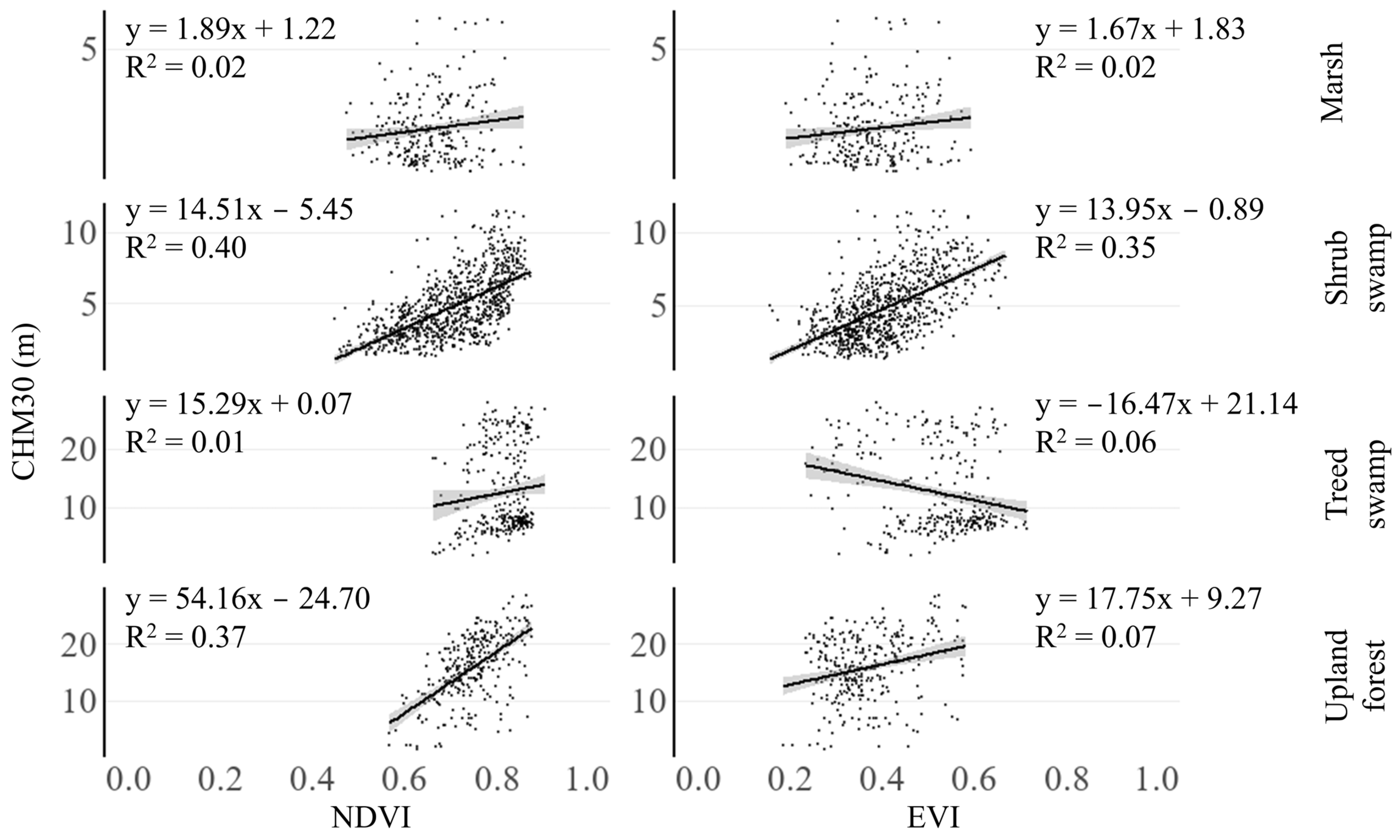
3.1. Correspondence Between Canopy Height and VIs

Figure 4 illustrates CHM5 for years 2000, 2016 and 2018 classified into four canopy height classes. Trees associated with CHM > 10 m tend to be upland forest classes and are located on terraces or elevated levees. This figure also shows the areal coverage of each canopy height class within surveyed areas A, B, C and D. From 2000 to 2018, there was a general increase in all categories of canopy height exceeding 1 m, with 52.8% of total land surface cover in 2000 compared to 66.2% for 2016–18.

Based on the distribution of random points (excluding marsh areas with vegetation <1 m) illustrated in

Table 1. Spearman correlation results between CHM30 and Landsat VIs for 2016/18 over the main landcover classes.

Landcover Class	N	Correlation with CHM30		p-Value
		NDVI	EVI	NDVI	EVI
Marsh	261	0.05	0.11	0.425	0.090
Shrub swamp	881	0.65 **	0.59 **	<0.001	<0.001
Treed swamp	292	0.13 *	−0.14 *	0.023	0.014
Upland forest	293	0.58 **	0.22 **	<0.001	<0.001
All	1727	0.63 **	0.31 **	<0.001	<0.001

** Correlation is significant at the 0.01 level (2-tailed). * Correlation is significant at the 0.05 level (2-tailed).

, both NDVI and EVI demonstrated a statistically significant correlation with CHM30, with greater correspondence to NDVI. Highest correlations between canopy height and vegetation indices were found in shrub swamp and upland forest, whereas treed swamp and marsh had much lower correspondence (Table 1, Figure 5). Confidence intervals (Figure 5) also demonstrate higher confidence and lower variability, especially in shrub swamps relative to other landcovers. The corresponding linear regression relationships show similar results and are presented in Figure 5. In shrub swamps, the 95% confidence intervals (CI) in this figure are the narrowest among the landcover classes for both NDVI and EVI, suggesting higher confidence in the trends.

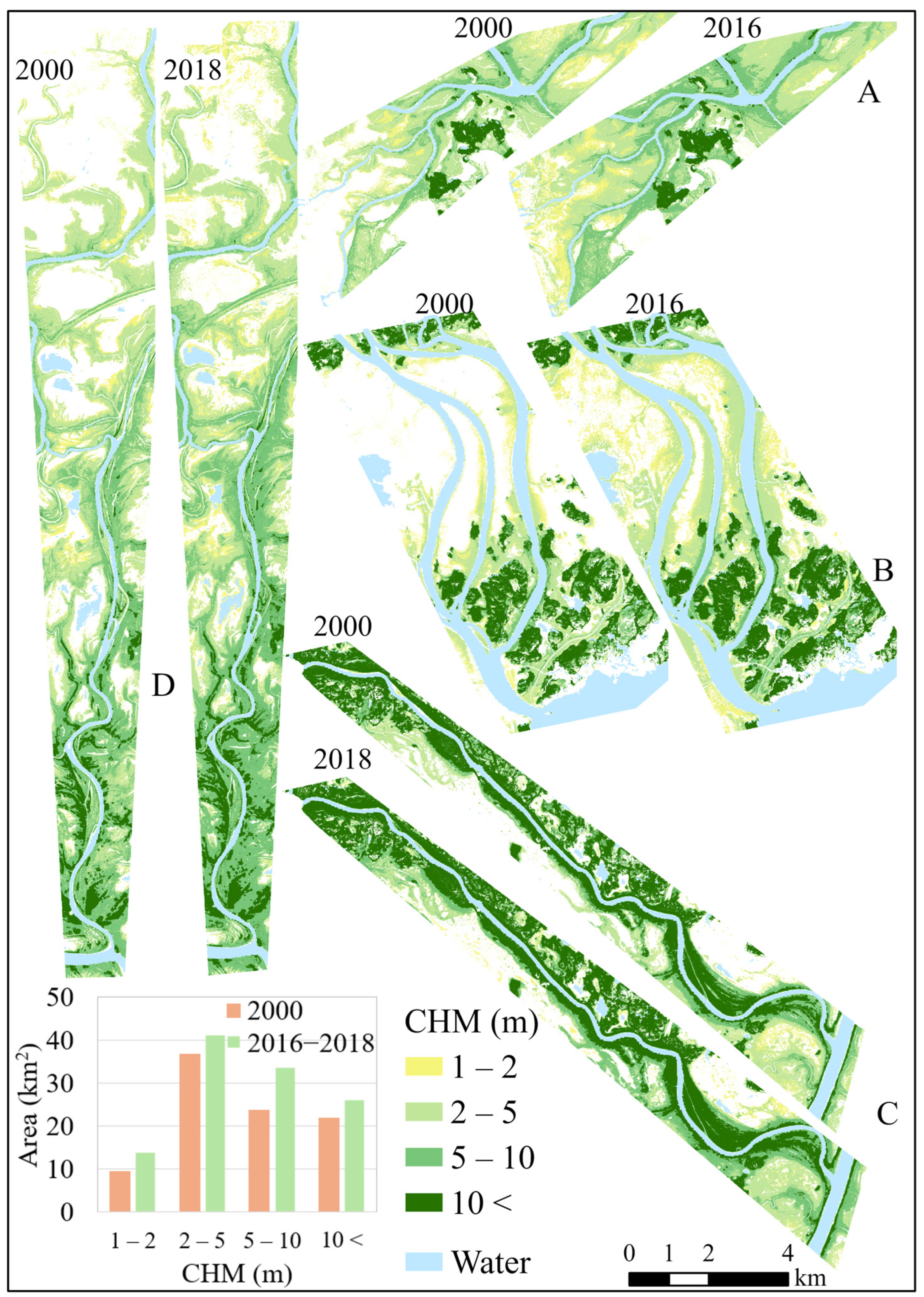
3.2. Changes in Canopy Height and Cover Using Bi-Temporal Lidar Data

Figure 6 presents the change in CHM30 (∆CHM30) from 2000 to 2016/18 over the four survey areas across five height change classes: large decrease (<−5 m), moderate decrease (−1 to −5 m), no appreciable change (−1 to 1 m), moderate increase (1 to 5 m), and large increase (>5 m). The landscape exhibited moderate canopy height growth over 55.8 km² (52.0% of land area after removing permanent open water and CHM < 1 m), and large increases in height over 4.9 km² (4.6% land area) indicating that the growth of taller (>1 m) vegetation has been the dominant trend, overall. In contrast, areas showing decreases in canopy height were comparatively small with large height decreases of 0.39 km² (0.4% land area) and moderate decrease of 3.7 km² (3.4% land area).

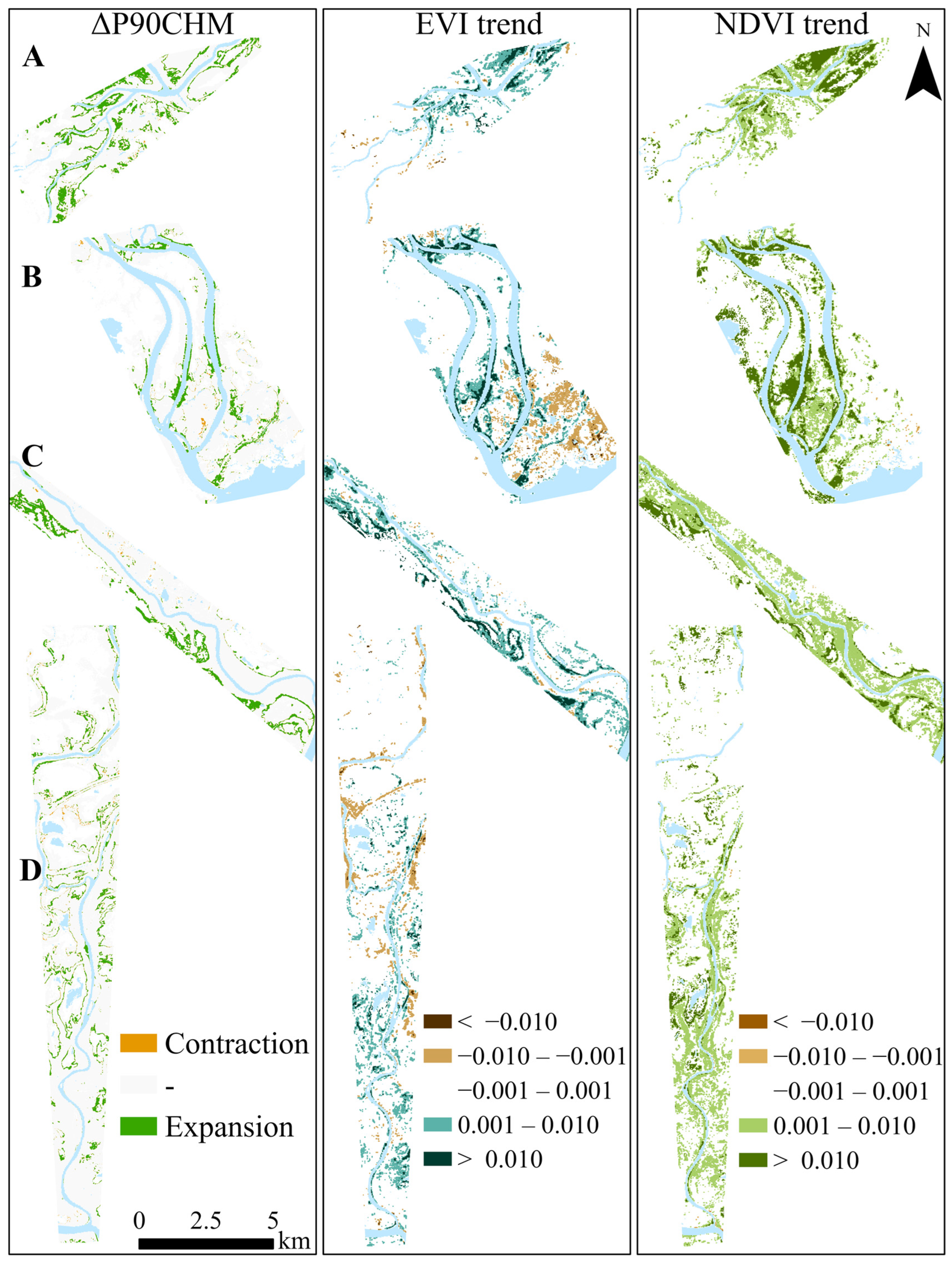
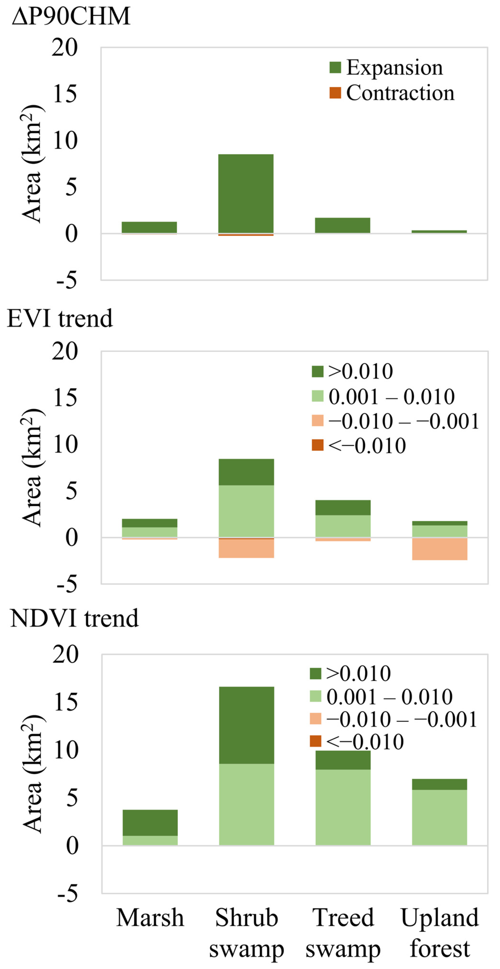
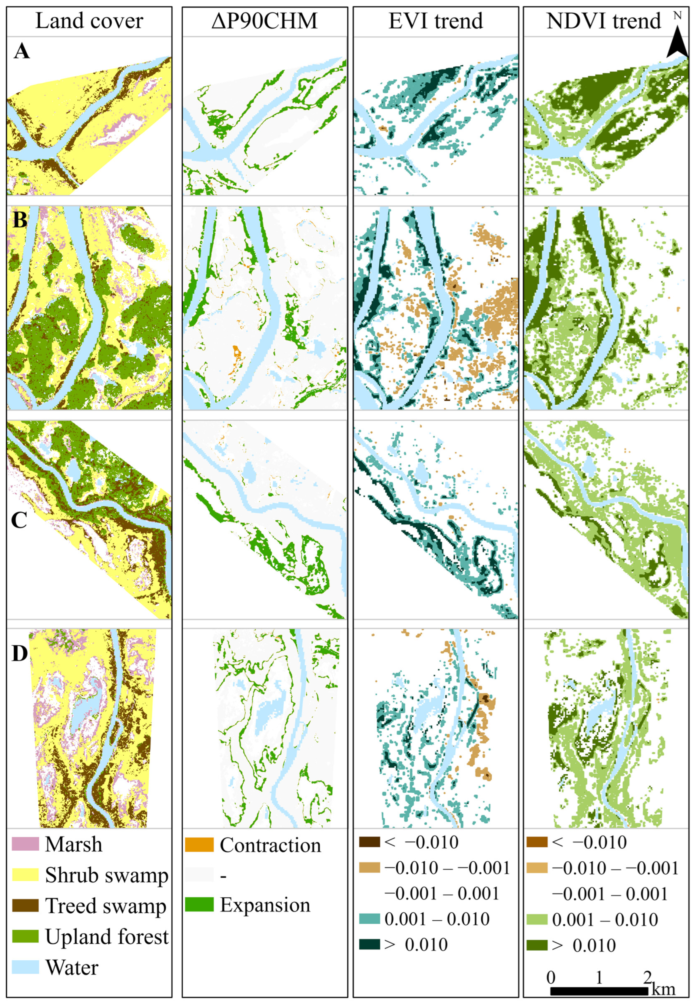
3.3. Changes in Ecotone Extent Inferred from CHM Change and VI Trend

Figure 7 shows the P90CHM change (∆P90CHM), EVI and NDVI trends (indicated by the Theil–Sen slope (p < 0.05). The analysis of significant VI trends indicated similar greening patterns to the ∆P90CHM expansion of woody ecotones, though the extents were variable. As illustrated in this figure across all four survey areas, the significant slopes for EVI display similar patterns to the observed height-based ecotonal expansions. Conversely, while NDVI also displays similar greening trends, the index overestimates the extent of greening relative to observed ecotonal expansions (Figure 7).

Stratifying ∆P90CHM by dominant landcover classes [68] (Figure 1) revealed that ~70% of ecotonal expansion (8.5 km²), equivalent to ~7% of the total survey area, occurred in shrub swamps (Figure 8). Meanwhile, treed swamps accounted for ~1.5% of the total expansion in the area. EVI exhibited negative slopes or browning predominantly in upland forest and shrub swamp (zoomed in example in Figure 9B), where no trend was present in the NDVI. This observed browning in the EVI trend, which encompasses a larger area (Figure 8), occasionally corresponds to the contraction of CHM in survey polygon B (Figure 7B), though the extent of the CHM-derived contraction is reduced. Most CHM expansion (Figure 8) occurred along the edge of shrub swamps (zoomed in examples in Figure 9A,C,D). In some cases, shrubs also extended into the marsh land class from adjacent swamps (Figure 9A,D). Moreover, comparing the observed ecotonal expansions with the most accurate landcover map provided by Wang, Pavelsky, Kyzivat, Garcia-Tigreros, Yao, Yang, Zhang, Song, Langhorst and Dolan [104] confirms that the expansions observed in our study predominantly occur over the dry shrub class identified in their study, which encompasses three of our four polygons (A, B and C).

Figure 9 shows zoomed-in examples of similarities and differences between products alongside the DUC landcover classes. In Figure 9A, although ∆P90CHM expansions were observed on the edges of treed swamp into shrub swamp and marsh, neither EVI nor NDVI reflected those exact expansions. Both NDVI and EVI positive slopes were observed over the inner parts of lowlands. However, when considering only larger positive EVI slope, more similarities with expansions in ∆P90CHM can be seen. NDVI here also showed small positive slopes over uplands. Some of the narrow contractions were reflected in EVI trends as small negatives. In Figure 9B, larger positive slopes of EVI were coordinated with the expansions in ∆P90CHM, over the treed swamp and shrub swamp on the levees. The larger positive NDVI slopes also showed the same pattern; however, the smaller positive NDVI slopes were seen over upland forest. In Figure 9C, ∆P90CHM expansions are limited to shrub swamps into marsh on the southern part of the stream. EVI positive slopes closely followed the same patterns observed in ∆P90CHM expansions. Similarly, these expansions were reflected as larger positive slopes in NDVI trend. Smaller positive slopes in NDVI covers almost all landcovers without any specific patterns. In Figure 9D, ∆P90CHM expansions were on the treed swamp into the shrub swamp around the marsh, with no sign of large contraction in this example. EVI positive slopes closely aligned with this expansion. Larger positive slopes in NDVI are more coordinated with the observed expansions. EVI also showed a small negative slope over some of the treed swamps in this example.

Comparing the ∆P90CHM through time suggests that >11% of the study area exhibited a change in forest ecotone extent, with ~11% showing expansion and ~0.3% contraction (Figure 8). The three Peace Delta polygons (A, B and C) demonstrated higher rates of forest ecotone change between 2.4 and 3.2 m/yr. Meanwhile, the more southerly Athabasca Delta polygon (D) displayed a slightly lower expansion rate of ~1.5 m/yr (

Table 2. t-test (independent samples, 2-tailed) between ΔP90CHM and VI trends per survey areas and overall rate of ecotonal expansion (m/yr).

Survey Area	ΔP90CHM	NDVI Trend	EVI Trend	ΔP90CHM vs. NDVI Trend		ΔP90CHM vs. EVI Trend
	Mean Rate of Expansion m/yr (SD)			Difference	p Value	Difference	p Value
A	3.3 (3.1)	5.5 (3.2)	2.4 (3.3)	−2.2	0.00	0.9	0.24
B	2.6 (3.0)	5.5 (5.0)	1.9 (3.0)	−2.9	0.00	0.7	0.39
C	2.4 (0.3)	7.2 (4.7)	3.6 (3.8)	−4.8	< 0.001	−1.2	0.04
D	1.5 (1.2)	4.1 (2.7)	1.7 (3.3)	−2.6	< 0.001	−0.2	0.62
All	2.2 (2.3)	5.4 (4.1)	2.3 (3.8)	−3.2	< 0.001	−0.1	0.79

SD: Standard Deviation.

). In all surveyed polygons, the regions of ecotonal expansion inferred from NDVI greening trends were greater than for areas of CHM increase (p < 0.05). The mean difference between ∆P90CHM and NDVI slope ranged from −2.2 to −4.9 units, indicating that NDVI consistently exhibited larger changes. In contrast, no significant difference was found between ∆P90CHM and EVI significant slope in most areas (A, B, D and overall), except for area C, where EVI changes were significantly greater than CHM (p = 0.040). Overall, the results show that NDVI greening rate was notably larger compared to ∆P90CHM, while ∆P90CHM and EVI significant slope exhibit similar expansion/greening rates in most areas. The average vertical rate of growth over the four survey areas is 0.1 m/yr.

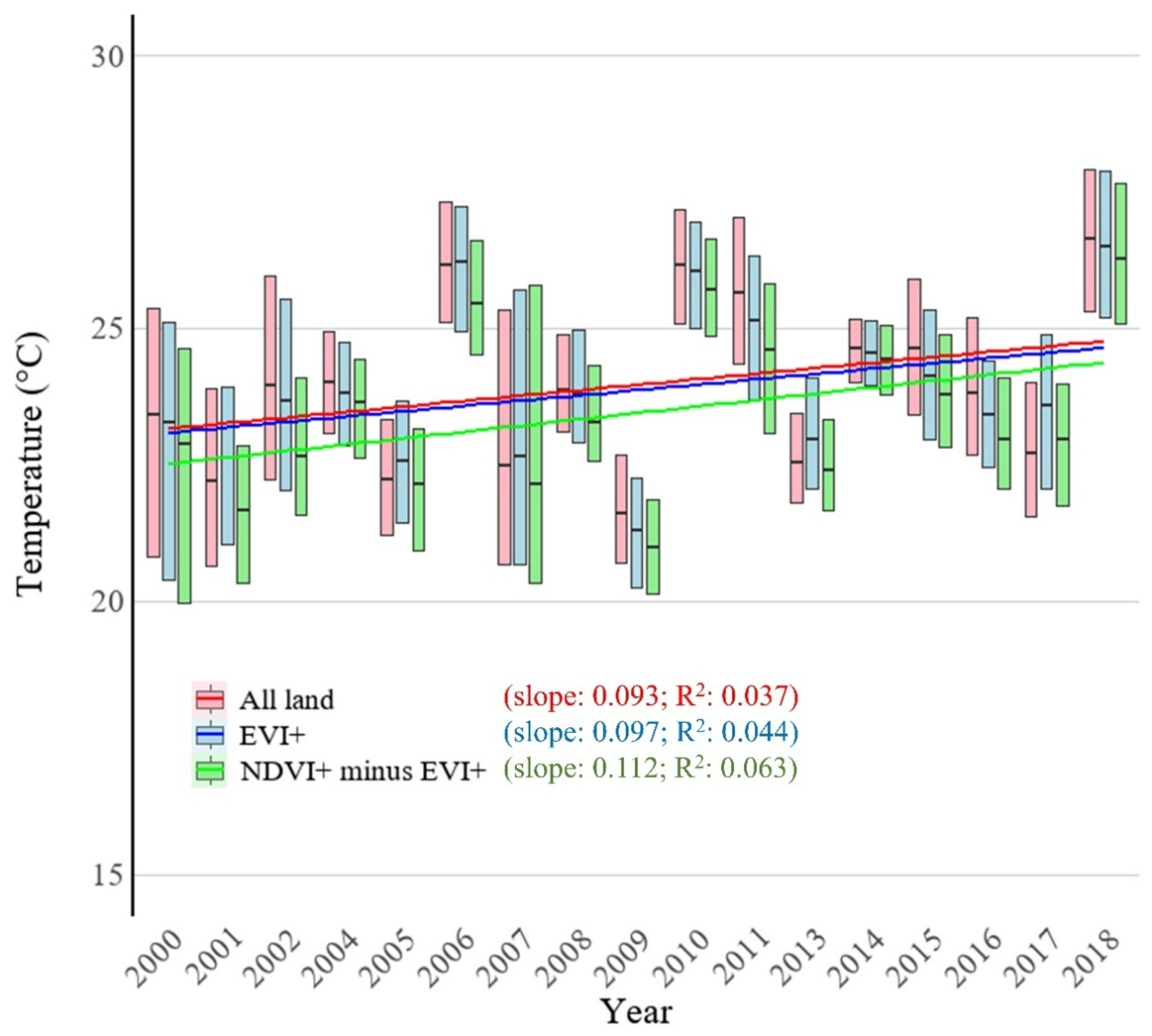
3.4. Changes in LST with VIs

Summertime Landsat-derived LST (°C) for all non-permanent water (all land) provided a baseline for comparison to (a) areas of significant (p < 0.05) TS greening for EVI (EVI+) and (b) areas of no EVI greening but significant NDVI greening (NDVI+ minus EVI+) (Figure 10). Only positive trends were considered here, as browning trends constituted a negligible proportion of the study area. All three trendlines (p < 0.001) show increasing LST. The “all land” (red) baseline condition exhibits the warmest temperatures throughout, with a slight warming trend of 1.67 °C per 18 yrs (slope: 0.093 °C/yr). In comparison, the EVI+ (blue) trendline lies slightly below the baseline condition but follows a similar warming pattern with a slightly non-significant trend difference of 1.74 °C per 18 yrs (slope: 0.097/yr). Areas showing only NDVI greening (NDVI+ minus EVI+ green line) were ~1 °C colder than either the baseline or EVI greening areas, but the rate of warming over exclusively NDVI greening areas was significantly greater at 2.02 °C per 18 yrs (slope: 0.11 °C/yr).

4. Discussion

4.1. Do EVI and NDVI Correlate with Canopy Height?

In this section, we explore the first objective that EVI, due to its assumed sensitivity to canopy structure and density, would demonstrate stronger positive correlations with CHM compared to NDVI—an expectation challenged by our findings. Of the two VIs, NDVI exhibited higher static correlations with CHM30 (a joint measure of height and cover) (Table 1) across all classes. This corroborates the findings from Taddeo et al. [106] where several VIs were compared over wetland sites in the US.

To address the second sub objective—supported by the different performance of NDVI and EVI across the examined classes—we found that the most notable divergent response between the VIs was in the upland forest class (Table 1) where NDVI showed a significantly stronger correlation with mean canopy height (r 0.58, p < 0.01) than EVI (r 0.22, p > 0.05). This finding indicates NDVI increases either as woody biomass grows taller, or when the gaps between taller woody vegetation fill in.

Of the landcovers examined, EVI only showed a highly significant correlation with shrubs (r = 0.59, p < 0.01), which was almost as high as NDVI (r = 0.63, p < 0.01), indicating that EVI was less responsive to canopy structure variations in tall tree (primarily conifer) environments. Shadow effects are expected to influence the spectral response of NDVI and EVI in taller vegetation areas, with inclusion of the blue band making EVI more susceptible to visible light variations caused by shadows (as reported by Moura et al. [107]). While inclusion of the blue band in EVI helps mitigate against saturation [34,35], the vegetation canopy cover in the PAD rarely approaches saturation in either VI, suggesting that for total foliage variations within northern environment tall woody vegetation classes, the benefits of EVI do not exceed NDVI.

Furthermore, woody vegetation generally exhibits lower reflectance in visible bands compared to herbaceous species [108], which could contribute to the lower EVI sensitivity to height and cover variations observed in taller forest vegetation classes. Chen et al. [109] reported a negative correlation between IKONOS-derived EVI and forest cover measures of effective LAI. High susceptibility of EVI to the effects of shadows, viewing and illumination geometry were also reported by Galvão et al. [110], Morton et al. [111], Galvão et al. [112], Taddeo, Dronova and Depsky [106] and Mo et al. [113].

This contrast in shadow sensitivity between NDVI and EVI underscores the importance of selecting appropriate indices based on specific environmental conditions and the physical characteristics of the vegetation. However, both NDVI and EVI demonstrated their strongest correlations with canopy cover in shrub swamps (Table 1, r = 0.65 and r = 0.59, respectively). The high correlation between canopy cover and VI likely reflects the dense and uniform vegetation typical of shrub swamps, where both indices are effective in capturing the biomass and structure due to limited soil and water interference that influence spectral response.

4.2. Do Temporal Trends in EVI and NDVI Correlate with Canopy Growth?

This section focuses on the second objective, which explores the spatial relationships between changes in CHM and VI trends, particularly in ecotonal areas where increases or decreases in height and foliage are most pronounced, such as those linked to woody vegetation expansion. Pervasive growth across the four study polygons from 2000 to 2016/18 is clear in the ∆CHM30 data presented in Figure 6. The range in canopy growth or loss dynamics is captured in five distinct canopy height change classes showing that, overall, >50% of the study area (55.9 km²) had undergone an average canopy height increase of >1 m, suggesting growth through mechanisms of either (a) in situ vertical stem extension, (b) in-filling of canopy gaps by crown expansion and new growth, (c) succession or lateral expansion of taller canopy cover outwards from woody ecotones or (d) some combination of all.

In areas of pre-existing woody cover classes, processes of in situ growth and in-filling of canopy gaps were likely the main mechanisms contributing to increases in overall CHM30. However, lateral expansion of primarily shrub and juvenile tree ecotones, observed using ∆P90CHM (Figure 7), indicated that >11% of the study area had undergone a change in vegetation cover because of ecotonal expansion. While almost 90% of the study area showed no discernible expansion or contraction of ecotones, the northern Peace Delta sector (areas A, B and C) exhibited higher rates of woody vegetation ecotone expansion between 2.4 and 3.2 m/yr (Table 2). This rapid expansion highlights a dynamic ecological response, driven by local environmental factors [114]. In contrast, the more southerly Athabasca Delta sector (area D) demonstrated a lower ecotone expansion rate closer to half that of the Peace Delta sites at ~1.5 m/yr, suggesting some differentiation in the underlying processes driving the expansion of woody ecotones across these two regions. From the limited spatial extent of the survey polygons, it cannot be concluded that the driving mechanisms for ecotone expansion are distinct. However, it is noteworthy that the three northern polygons lie along channels that have historically reversed in flow direction [115], while the southern polygon is along a channel that naturally drains in one direction. Consequently, local channel and floodplain physiography and hydrology play a role in the patterns and rates of vegetation encroachment [8,65]. For example, surveyed area C, situated at a higher elevation above the main waterways, likely depends on ice-jam floodwater input, which has been less frequent in the Peace Delta compared to the Athabasca Delta between 2000 and 2018. In contrast, surveyed area B is located within a low-lying floodplain that expands with water during periods of elevated Lake Athabasca levels [116].

As expected from the positive correlations of VI with canopy height, and as reported in other northern studies [23,53,117] greening (or increasingly positive) trends were observed in both EVI and NDVI across the study sites. Unlike in the direct correlation between VI and canopy height, the spatial correspondence between VI greening and increasing canopy height was most pronounced in the EVI signal. Notably, the most significant areas of EVI greening tend to visually align with and show a similar rate of spatial extent variations in woody ecotones defined using ∆P90CHM (the change in upper canopy height percentile) (Figure 8 and Figure 9, Table 2). Meanwhile, NDVI greening shows less direct correspondence and suggests a higher rate of woody ecotone expansion, while being more sensitive to a wider range of vegetation changes. These observations indicate that NDVI captures a spatially broader range of vegetation response, including shorter stature vegetation, compared to that in the CHM-based analyses.

Greater areas of observed NDVI greening may be influenced by the sensitivity of the NDVI to changes in vegetation type or differences in spatial resolution between Landsat and lidar-derived products. Other studies have reported an overestimation in NDVI greening trends, which could be unrelated to in situ vegetation structural properties. Over different land covers within a semi-arid to arid region of northwest China, Gao et al. [118] attributed NDVI overestimation or underestimation to spatial resolution (250 m MODIS and 8 km GIMMS). Vicente-Serrano et al. [119] also found an overestimation of greening trends when using NDVI to detect vegetation change at 1 km resolution. Given some potential for overestimation, it is important to consider the magnitude and extent of the observed NDVI greening. NDVI is derived through a non-linear transformation, which can lead to the overestimation of NDVI values in areas with low vegetation coverage and underestimation in areas with high vegetation coverage [20]. It can be assumed that any systematic overestimation in NDVI would persist throughout the entire study period, suggesting that temporal variations in NDVI should be minimally impacted [120].

EVI also demonstrated some areas of negative slope (browning), in some upland forest landcover areas, while the NDVI trends showed greening throughout the survey polygons. The observation of loss or contraction in the EVI slope signal is encouraging because it matches the observation for ∆P90CHM woody ecotone contraction. However, there was limited direct spatial correspondence between the two losses (e.g., Figure 9), indicating that both the EVI and ∆P90CHM observations, while synergistic, are responding to subtly distinct in situ ground-level processes. Several studies have overlooked the classification of EVI browning in northern latitudes, attributing its exclusion to its occurrence over relatively small areas (e.g., Chen, Lantz, Hermosilla and Wulder [22]; Seider, Lantz, Hermosilla, Wulder and Wang [23]). Other researchers have documented EVI browning in boreal forests (e.g., Guay, Beck, Berner, Goetz, Baccini and Buermann [24]; Lebre [25]) with a suggestion that increases in surface water presence is a likely cause [121].

4.3. How Do Trends in LST Differ Between EVI and NDVI Trends?

In Figure 10, all three LST trendlines (p < 0.001) show increasing LST, which is consistent with a gradual reduction in evaporative latent heat exchanges as areas of open water and surface soil saturation decrease, ground water tables deepen, and conditions become drier overall [101,102]. Among the three trendlines (Figure 10), areas showing only NDVI greening (NDVI+ minus EVI+ green line) exhibited the lowest and fastest warming rate. The lower temperatures suggest that these areas of exclusive NDVI greening are associated with increased wetness, while the more rapid increase in warming suggests a drying trend, where regions of high moisture content (e.g., wetlands or areas of high water table) have undergone more rapid warming as they dry out. The NDVI response to this drying out of wetland and wetland-adjacent areas is likely a function of both the changes in surface moisture content having some influence on the NIR signal [122], as well as the ground cover vegetation response as saturation-tolerant vegetation in marsh areas is replaced with more dryland vegetation [8].

In this northern deltaic wetland study area, positive EVI trends tend to primarily illustrate ecotonal expansions in areas of shrub and juvenile tree cover, while negative EVI trends may correctly indicate the potential for canopy losses, if not the precise locations. Meanwhile, spatial variations in NDVI trends appear sensitive to both changes in tall vegetation canopy height (Figure 5) and as has been found in other studies, temporal changes in ground surface moisture [123,124,125,126].

To synthesize these findings, Figure 11 presents a conceptual framework illustrating the complementary insights provided by VIs, LST and MNDWI. As surface moisture content decreases due to drying (e.g., reduced soil saturation), less energy is allocated to latent heat processes (evaporation), and land surface sensible heat content rises, leading to localized increases in LST. This warming is pronounced in areas undergoing transition from saturated or near-saturated conditions to dry, such as over short vegetation zones, where surface moisture content directly influences LST. Conversely, areas with consistent tree canopy cover are less affected, as the canopy masks variations in surface temperature. The conceptual model emphasizes that positive LST trends are primarily observable in open or short vegetation areas, where drying and warming processes are not obscured by dense canopy cover. NDVI and EVI are complimentary in this model, with NDVI indicating general vegetation greening (both short and tall vegetation) as well as an increased sensitivity to changing surface saturation, while EVI better represents ecosystem structural changes associated with woody ecotonal expansion, such as shrubification. Meanwhile, MNDWI tracks reductions in surface water extent, thus completing a conceptual remote sensing-based narrative of land surface and cover changes through time across northern wetland complexes, like the PAD.

5. Conclusions

The findings from this study underscore the importance of selecting appropriate vegetation indices tailored to specific environmental conditions and vegetation characteristics in wetland ecosystems—an issue of growing global relevance as wetland monitoring becomes increasingly critical in the context of climate change and biodiversity loss. Both NDVI and EVI showed the highest correlation with canopy height and cover (CHM30) over shrub swamps, with NDVI being more sensitive to canopy height variation in all woody vegetation classes. However, the strength and direction of CHM–VI relationships varied across landcover types, reflecting the differing sensitivity of each index to vegetation structure and moisture conditions in each class. While NDVI tends to capture a broader range of vegetation responses, including shorter stature vegetation, its potential for over-estimating the time-variant greening response of a landscape due to the sensitivity to changes in canopy structure or surface moisture cannot be ignored. EVI exhibited more spatially consistent trends in areas of taller woody canopy, making it more suitable for detecting ecotonal expansion and succession in structurally complex wetland zones. In contrast, NDVI trends were more responsive to vegetation changes in lower-stature, moisture-sensitive areas, particularly where wetland drying was observed. These findings highlight the complementary strengths of NDVI and EVI in capturing different aspects of wetland vegetation change, offering insight into both structural canopy shifts and surface moisture responses. In particular, the as yet inconclusive evidence we present here for comparatively increased rates of woody ecotonal expansion in the historically reversible flow areas of the Peace Delta warrants dedicated investigation. The conceptual framework presented in Figure 11 provides a basis for a multi-decadal assessment of wetland open water, surface moisture and vegetation canopy change. While developed for the PAD, it offers a transferable approach that can inform similar assessments in other northern wetland complexes worldwide, contributing to international efforts in wetland conservation and climate adaptation.

References

1. Timoney, K.; La Roi, G.; Zoltai, S.; Robinson, A. The high subarctic forest-tundra of northwestern Canada: Position, width, and vegetation gradients in relation to climate. Arctic 1992, 45, 1–9. [Google Scholar] [CrossRef]
2. Ecosystem Classification Group. Ecological Regions of the Northwest Territories–Taiga Plains; Department of Environment and Natural Resources, Government of Northwest Territories: Yellowknife, NT, Canada, 2007.
3. Fu, L.; Xie, R.; Ma, D.; Zhang, M.; Liu, L. Variations in soil microbial community structure and extracellular enzymatic activities along a forest–wetland ecotone in high-latitude permafrost regions. Ecol. Evol. 2023, 13, e10205. [Google Scholar] [CrossRef] [PubMed]
4. Dimitrov, D.D.; Bhatti, J.S.; Grant, R.F. The transition zones (ecotone) between boreal forests and peatlands: Ecological controls on ecosystem productivity along a transition zone between upland black spruce forest and a poor forested fen in central Saskatchewan. Ecol. Model. 2014, 291, 96–108. [Google Scholar] [CrossRef]
5. Lieffers, V.J.; Rothwell, R.L. Rooting of peatland black spruce and tamarack in relation to depth of water table. Can. J. Bot. 1987, 65, 817–821. [Google Scholar] [CrossRef]
6. Grant, R.F. Modeling topographic effects on net ecosystem productivity of boreal black spruce forests. Tree Physiol. 2004, 24, 1–18. [Google Scholar] [CrossRef]
7. Gower, S.T.; Vogel, J.G.; Norman, J.M.; Kucharik, C.J.; Steele, S.J.; Stow, T.K. Carbon distribution and aboveground net primary production in aspen, jack pine, and black spruce stands in Saskatchewan and Manitoba, Canada. J. Geophys. Res. Atmos. 1997, 102, 29029–29041. [Google Scholar] [CrossRef]
8. Timoney, K.P. The Peace-Athabasca Delta: Portrait of a Dynamic Ecosystem; University of Alberta: Edmonton, AB, Canada, 2013. [Google Scholar]
9. Enayetullah, H.; Chasmer, L.; Hopkinson, C.; Thompson, D.; Cobbaert, D. Identifying Conifer Tree vs. Deciduous Shrub and Tree Regeneration Trajectories in a Space-for-Time Boreal Peatland Fire Chronosequence Using Multispectral Lidar. Atmosphere 2022, 13, 112. [Google Scholar] [CrossRef]
10. Jean, S.A.; Pinno, B.D.; Nielsen, S.E. Early regeneration dynamics of pure black spruce and aspen forests after wildfire in boreal Alberta, Canada. Forests 2020, 11, 333. [Google Scholar] [CrossRef]
11. Mitsch, W.J.; Gosselink, J.G. Wetlands; John Wiley & Sons: Hoboken, NJ, USA, 2015. [Google Scholar]
12. Carpino, O.A.; Berg, A.A.; Quinton, W.L.; Adams, J.R. Climate change and permafrost thaw-induced boreal forest loss in northwestern Canada. Environ. Res. Lett. 2018, 13, 084018. [Google Scholar] [CrossRef]
13. Birch, J.D.; Lutz, J.A.; Hogg, E.H.; Simard, S.W.; Pelletier, R.; LaRoi, G.H.; Karst, J. Decline of an ecotone forest: 50 years of demography in the southern boreal forest. Ecosphere 2019, 10, e02698. [Google Scholar] [CrossRef]
14. Tremblay, B.; Lévesque, E.; Boudreau, S. Recent expansion of erect shrubs in the Low Arctic: Evidence from Eastern Nunavik. Environ. Res. Lett. 2012, 7, 035501. [Google Scholar] [CrossRef]
15. Frost, G.V.; Epstein, H.E. Tall shrub and tree expansion in Siberian tundra ecotones since the 1960s. Glob. Change Biol. 2014, 20, 1264–1277. [Google Scholar] [CrossRef] [PubMed]
16. Jackson, M.M.; Topp, E.; Gergel, S.E.; Martin, K.; Pirotti, F.; Sitzia, T. Expansion of subalpine woody vegetation over 40 years on Vancouver Island, British Columbia, Canada. Can. J. For. Res. 2016, 46, 437–443. [Google Scholar] [CrossRef]
17. Chasmer, L.; Cobbaert, D.; Mahoney, C.; Millard, K.; Peters, D.; Devito, K.; Brisco, B.; Hopkinson, C.; Merchant, M.; Montgomery, J.; et al. Remote Sensing of Boreal Wetlands 1: Data Use for Policy and Management. Remote Sens. 2020, 12, 1320. [Google Scholar] [CrossRef]
18. Töyrä, J.; Pietroniro, A. Towards operational monitoring of a northern wetland using geomatics-based techniques. Remote Sens. Environ. 2005, 97, 174–191. [Google Scholar] [CrossRef]
19. Tucker, C.J. Red and photographic infrared linear combinations for monitoring vegetation. Remote Sens. Environ. 1979, 8, 127–150. [Google Scholar] [CrossRef]
20. Huete, A.; Liu, H.; Batchily, K.; Van Leeuwen, W. A comparison of vegetation indices over a global set of TM images for EOS-MODIS. Remote Sens. Environ. 1997, 59, 440–451. [Google Scholar] [CrossRef]
21. Huete, A.; Justice, C.; Liu, H. Development of vegetation and soil indices for MODIS-EOS. Remote Sens. Environ. 1994, 49, 224–234. [Google Scholar] [CrossRef]
22. Chen, A.; Lantz, T.C.; Hermosilla, T.; Wulder, M.A. Biophysical controls of increased tundra productivity in the western Canadian Arctic. Remote Sens. Environ. 2021, 258, 112358. [Google Scholar] [CrossRef]
23. Seider, J.H.; Lantz, T.C.; Hermosilla, T.; Wulder, M.A.; Wang, J.A. Biophysical determinants of shifting tundra vegetation productivity in the Beaufort Delta region of Canada. Ecosystems 2022, 25, 1435–1454. [Google Scholar] [CrossRef]
24. Guay, K.C.; Beck, P.S.A.; Berner, L.T.; Goetz, S.J.; Baccini, A.; Buermann, W. Vegetation productivity patterns at high northern latitudes: A multi-sensor satellite data assessment. Glob. Change Biol. 2014, 20, 3147–3158. [Google Scholar] [CrossRef] [PubMed]
25. Lebre, D. Differences in Vegetation Composition and Structure at Greening and Non-Greening Sites in the Northwest Territories. Ph.D. Thesis, Queen’s University, Ontario, CA, Canada, 2019. [Google Scholar]
26. Morawitz, D.F.; Blewett, T.M.; Cohen, A.; Alberti, M. Using NDVI to Assess Vegetative Land Cover Change in Central Puget Sound. Environ. Monit. Assess. 2006, 114, 85–106. [Google Scholar] [CrossRef] [PubMed]
27. Martinez, A.D.l.I.; Labib, S.M. Demystifying normalized difference vegetation index (NDVI) for greenness exposure assessments and policy interventions in urban greening. Environ. Res. 2023, 220, 115155. [Google Scholar] [CrossRef]
28. Leahy, M.G.; Jollineau, M.Y.; Howarth, P.J.; Gillespie, A.R. The use of Landsat data for investigating the long-term trends in wetland change at Long Point, Ontario. Can. J. Remote Sens. 2005, 31, 240–254. [Google Scholar] [CrossRef]
29. Olthof, I.; Pouliot, D.; Latifovic, R.; Chen, W. Recent (1986–2006) vegetation-specific NDVI trends in northern Canada from satellite data. Arctic 2008, 61, 381–394. [Google Scholar] [CrossRef]
30. Matsushita, B.; Yang, W.; Chen, J.; Onda, Y.; Qiu, G. Sensitivity of the Enhanced Vegetation Index (EVI) and Normalized Difference Vegetation Index (NDVI) to Topographic Effects: A Case Study in High-density Cypress Forest. Sensors 2007, 7, 2636–2651. [Google Scholar] [CrossRef]
31. Garroutte, E.L.; Hansen, A.J.; Lawrence, R.L. Using NDVI and EVI to Map Spatiotemporal Variation in the Biomass and Quality of Forage for Migratory Elk in the Greater Yellowstone Ecosystem. Remote Sens. 2016, 8, 404. [Google Scholar] [CrossRef]
32. Birky, A.K. NDVI and a simple model of deciduous forest seasonal dynamics. Ecol. Model. 2001, 143, 43–58. [Google Scholar] [CrossRef]
33. Sellers, P.J. Canopy reflectance, photosynthesis and transpiration. Int. J. Remote Sens. 1985, 6, 1335–1372. [Google Scholar] [CrossRef]
34. Huete, A.; Didan, K.; Miura, T.; Rodriguez, E.P.; Gao, X.; Ferreira, L.G. Overview of the radiometric and biophysical performance of the MODIS vegetation indices. Remote Sens. Environ. 2002, 83, 195–213. [Google Scholar] [CrossRef]
35. Liu, H.Q.; Huete, A. A feedback based modification of the NDVI to minimize canopy background and atmospheric noise. IEEE Trans. Geosci. Remote Sens. 1995, 33, 457–465. [Google Scholar] [CrossRef]
36. Sesnie, S.E.; Dickson, B.G.; Rosenstock, S.S.; Rundall, J.M. A comparison of Landsat TM and MODIS vegetation indices for estimating forage phenology in desert bighorn sheep (Ovis canadensis nelsoni) habitat in the Sonoran Desert, USA. Int. J. Remote Sens. 2012, 33, 276–286. [Google Scholar] [CrossRef]
37. Berner, L.T.; Goetz, S.J. Satellite observations document trends consistent with a boreal forest biome shift. Glob. Change Biol. 2022, 28, 3275–3292. [Google Scholar] [CrossRef] [PubMed]
38. Eastman, J.R.; Sangermano, F.; Machado, E.A.; Rogan, J.; Anyamba, A. Global trends in seasonality of normalized difference vegetation index (NDVI), 1982–2011. Remote Sens. 2013, 5, 4799–4818. [Google Scholar] [CrossRef]
39. Han, Y.; Wang, Y.; Zhao, Y. Estimating soil moisture conditions of the greater Changbai Mountains by land surface temperature and NDVI. IEEE Trans. Geosci. Remote Sens. 2010, 48, 2509–2515. [Google Scholar]
40. Naga Rajesh, A.; Abinaya, S.; Purna Durga, G.; Lakshmi Kumar, T.V. Long-term relationships of MODIS NDVI with rainfall, land surface temperature, surface soil moisture and groundwater storage over monsoon core region of India. Arid Land Res. Manag. 2023, 37, 51–70. [Google Scholar] [CrossRef]
41. Thiebault, K.; Young, S. Snow cover change and its relationship with land surface temperature and vegetation in northeastern North America from 2000 to 2017. Int. J. Remote Sens. 2020, 41, 8453–8474. [Google Scholar] [CrossRef]
42. Sharma, M.; Bangotra, P.; Gautam, A.S.; Gautam, S. Sensitivity of normalized difference vegetation index (NDVI) to land surface temperature, soil moisture and precipitation over district Gautam Buddh Nagar, UP, India. Stoch. Environ. Res. Risk Assess. 2022, 36, 1779–1789. [Google Scholar] [CrossRef]
43. Raynolds, M.K.; Comiso, J.C.; Walker, D.A.; Verbyla, D. Relationship between satellite-derived land surface temperatures, arctic vegetation types, and NDVI. Remote Sens. Environ. 2008, 112, 1884–1894. [Google Scholar] [CrossRef]
44. Kim, J.; Hogue, T.S. Improving spatial soil moisture representation through integration of AMSR-E and MODIS products. IEEE Trans. Geosci. Remote Sens. 2011, 50, 446–460. [Google Scholar] [CrossRef]
45. Zhang, F.; Zhang, L.-W.; Shi, J.-J.; Huang, J.-F. Soil Moisture Monitoring Based on Land Surface Temperature-Vegetation Index Space Derived from MODIS Data. Pedosphere 2014, 24, 450–460. [Google Scholar] [CrossRef]
46. Kornelsen, K.C.; Coulibaly, P. Advances in soil moisture retrieval from synthetic aperture radar and hydrological applications. J. Hydrol. 2013, 476, 460–489. [Google Scholar] [CrossRef]
47. Joshi, N.; Baumann, M.; Ehammer, A.; Fensholt, R.; Grogan, K.; Hostert, P.; Jepsen, M.R.; Kuemmerle, T.; Meyfroidt, P.; Mitchard, E.T.A.; et al. A Review of the Application of Optical and Radar Remote Sensing Data Fusion to Land Use Mapping and Monitoring. Remote Sens. 2016, 8, 70. [Google Scholar] [CrossRef]
48. Hopkinson, C.; Chasmer, L.E.; Sass, G.; Creed, I.F.; Sitar, M.; Kalbfleisch, W.; Treitz, P. Vegetation class dependent errors in lidar ground elevation and canopy height estimates in a boreal wetland environment. Can. J. Remote Sens. 2005, 31, 191–206. [Google Scholar] [CrossRef]
49. Wulder, M.A.; White, J.C.; Bater, C.W.; Coops, N.C.; Hopkinson, C.; Chen, G. Lidar plots—A new large-area data collection option: Context, concepts, and case study. Can. J. Remote Sens. 2012, 38, 600–618. [Google Scholar] [CrossRef]
50. Montgomery, J.; Brisco, B.; Chasmer, L.; Devito, K.; Cobbaert, D.; Hopkinson, C. SAR and LiDAR temporal data fusion approaches to boreal wetland ecosystem monitoring. Remote Sens. 2019, 11, 161. [Google Scholar] [CrossRef]
51. Rood, S.B.; Kaluthota, S.; Philipsen, L.J.; Slaney, J.; Jones, E.; Chasmer, L.; Hopkinson, C. Camo-maps: An efficient method to assess and project riparian vegetation colonization after a major river flood. Ecol. Eng. 2019, 141, 105610. [Google Scholar] [CrossRef]
52. Chasmer, L.; Mahoney, C.; Millard, K.; Nelson, K.; Peters, D.; Merchant, M.; Hopkinson, C.; Brisco, B.; Niemann, O.; Montgomery, J. Remote sensing of boreal wetlands 2: Methods for evaluating boreal wetland ecosystem state and drivers of change. Remote Sens. 2020, 12, 1321. [Google Scholar] [CrossRef]
53. Bolton, D.K.; Coops, N.C.; Hermosilla, T.; Wulder, M.A.; White, J.C. Evidence of vegetation greening at alpine treeline ecotones: Three decades of Landsat spectral trends informed by lidar-derived vertical structure. Environ. Res. Lett. 2018, 13, 084022. [Google Scholar] [CrossRef]
54. Hopkinson, C.; Sitar, M.; Chasmer, L.; Treitz, P. Mapping snowpack depth beneath forest canopies using airborne lidar. Photogramm. Eng. Remote Sens. 2004, 70, 323–330. [Google Scholar] [CrossRef]
55. Jones, E.A.; Chasmer, L.E.; Devito, K.J.; Hopkinson, C.D. Shortening fire return interval predisposes west-central Canadian boreal peatlands to more rapid vegetation growth and transition to forest cover. Glob. Change Biol. 2024, 30, e17185. [Google Scholar] [CrossRef] [PubMed]
56. Hopkinson, C.; Chasmer, L.; Barr, A.; Kljun, N.; Black, T.; McCaughey, J. Monitoring boreal forest biomass and carbon storage change by integrating airborne laser scanning, biometry and eddy covariance data. Remote Sens. Environ. 2016, 181, 82–95. [Google Scholar] [CrossRef]
57. Ji, P.; Su, R.; Wu, G.; Xue, L.; Zhang, Z.; Fang, H.; Gao, R.; Zhang, W.; Zhang, D. Projecting Future Wetland Dynamics Under Climate Change and Land Use Pressure: A Machine Learning Approach Using Remote Sensing and Markov Chain Modeling. Remote Sens. 2025, 17, 1089. [Google Scholar] [CrossRef]
58. Gxokwe, S.; Dube, T.; Mazvimavi, D. Multispectral Remote Sensing of Wetlands in Semi-Arid and Arid Areas: A Review on Applications, Challenges and Possible Future Research Directions. Remote Sens. 2020, 12, 4190. [Google Scholar] [CrossRef]
59. Pan, F.; Xie, J.; Lin, J.; Zhao, T.; Ji, Y.; Hu, Q.; Pan, X.; Wang, C.; Xi, X. Evaluation of Climate Change Impacts on Wetland Vegetation in the Dunhuang Yangguan National Nature Reserve in Northwest China Using Landsat Derived NDVI. Remote Sens. 2018, 10, 735. [Google Scholar] [CrossRef]
60. Ma, Z.; Chen, W.; Xiao, A.; Zhang, R. The Susceptibility of Wetland Areas in the Yangtze River Basin to Temperature and Vegetation Changes. Remote Sens. 2023, 15, 4534. [Google Scholar] [CrossRef]
61. Asner, G.P.; Clark, J.K.; Mascaro, J.; Vaudry, R.; Chadwick, K.D.; Vieilledent, G.; Rasamoelina, M.; Balaji, A.; Kennedy-Bowdoin, T.; Maatoug, L. Human and environmental controls over aboveground carbon storage in Madagascar. Carbon Balance Manag. 2012, 7, 2. [Google Scholar] [CrossRef]
62. Goetz, S.; Dubayah, R. Advances in remote sensing technology and implications for measuring and monitoring forest carbon stocks and change. Carbon Manag. 2011, 2, 231–244. [Google Scholar] [CrossRef]
63. Zhou, G.; Yin, X. Relationship of cotton nitrogen and yield with Normalized Difference Vegetation Index and plant height. Nutr. Cycl. Agroecosyst. 2014, 100, 147–160. [Google Scholar] [CrossRef]
64. Ramsar Convention. An Introduction to the Ramsar Convention on Wetlands, 7th ed. Available online: https://www.ramsar.org/sites/default/files/documents/library/handbook1_5ed_introductiontoconvention_final_e.pdf (accessed on 1 February 2024).
65. Peters, D.L.; Prowse, T.D.; Pietroniro, A.; Leconte, R. Flood hydrology of the Peace—Athabasca Delta, northern Canada. Hydrol. Process. Int. J. 2006, 20, 4073–4096. [Google Scholar] [CrossRef]
66. Peters, D.L.; Prowse, T.D.; Marsh, P.; Lafleur, P.M.; Buttle, J.M. Persistence of water within perched basins of the Peace-Athabasca Delta, Northern Canada. Wetl. Ecol. Manag. 2006, 14, 221–243. [Google Scholar] [CrossRef]
67. Newton, B.W.; Taube, N. Regional variability and changing water distributions drive large-scale water resource availability in Alberta, Canada. Can. Water Resour. J. Rev. Can. Ressour. Hydr. 2023, 48, 300–326. [Google Scholar] [CrossRef]
68. Ducks Unlimited Canada. Wood Buffalo National Park Enhanced Wetland Classification User’s Guide; Ducks Unlimited Canada: Edmonton, AB, Canada, 2020; p. 50. [Google Scholar]
69. Mishra, N.; Helder, D.; Barsi, J.; Markham, B. Continuous calibration improvement in solar reflective bands: Landsat 5 through Landsat 8. Remote Sens. Environ. 2016, 185, 7–15. [Google Scholar] [CrossRef] [PubMed]
70. Potapov, P.; Turubanova, S.; Hansen, M.C. Regional-scale boreal forest cover and change mapping using Landsat data composites for European Russia. Remote Sens. Environ. 2011, 115, 548–561. [Google Scholar] [CrossRef]
71. Roy, D.P.; Kovalskyy, V.; Zhang, H.; Vermote, E.F.; Yan, L.; Kumar, S.; Egorov, A. Characterization of Landsat-7 to Landsat-8 reflective wavelength and normalized difference vegetation index continuity. Remote Sens. Environ. 2016, 185, 57–70. [Google Scholar] [CrossRef]
72. Qiu, S.; Lin, Y.; Shang, R.; Zhang, J.; Ma, L.; Zhu, Z. Making Landsat time series consistent: Evaluating and improving Landsat analysis ready data. Remote Sens. 2018, 11, 51. [Google Scholar] [CrossRef]
73. Chen, S.; Woodcock, C.E.; Bullock, E.L.; Arévalo, P.; Torchinava, P.; Peng, S.; Olofsson, P. Monitoring temperate forest degradation on Google Earth Engine using Landsat time series analysis. Remote Sens. Environ. 2021, 265, 112648. [Google Scholar] [CrossRef]
74. Masek, J.G.; Wulder, M.A.; Markham, B.; McCorkel, J.; Crawford, C.J.; Storey, J.; Jenstrom, D.T. Landsat 9: Empowering open science and applications through continuity. Remote Sens. Environ. 2020, 248, 111968. [Google Scholar] [CrossRef]
75. USGS. Landsat Collection 2. Available online: https://pubs.usgs.gov/fs/2021/3002/fs20213002.pdf (accessed on 1 April 2024).
76. Töyrä, J.; Pietroniro, A.; Hopkinson, C.; Kalbfleisch, W. Assessment of airborne scanning laser altimetry (lidar) in a deltaic wetland environment. Can. J. Remote Sens. 2003, 29, 718–728. [Google Scholar] [CrossRef]
77. Hopkinson, C.; Chasmer, L.; Gynan, C.; Mahoney, C.; Sitar, M. Multisensor and Multispectral LiDAR Characterization and Classification of a Forest Environment. Can. J. Remote Sens. 2016, 42, 501–520. [Google Scholar] [CrossRef]
78. Hopkinson, C.; Chasmer, L.; Hall, R. The uncertainty in conifer plantation growth prediction from multi-temporal lidar datasets. Remote Sens. Environ. 2008, 112, 1168–1180. [Google Scholar] [CrossRef]
79. Lim, K.; Hopkinson, C.; Treitz, P. Examining the effects of sampling point densities on laser canopy height and density metrics. For. Chron. 2008, 84, 876–885. [Google Scholar] [CrossRef]
80. Crego, R.D.; Stabach, J.A.; Connette, G. Implementation of species distribution models in Google Earth Engine. Divers. Distrib. 2022, 28, 904–916. [Google Scholar] [CrossRef]
81. Hemati, M.; Hasanlou, M.; Mahdianpari, M.; Mohammadimanesh, F. A systematic review of landsat data for change detection applications: 50 years of monitoring the earth. Remote Sens. 2021, 13, 2869. [Google Scholar] [CrossRef]
82. Teluguntla, P.; Thenkabail, P.S.; Oliphant, A.; Xiong, J.; Gumma, M.K.; Congalton, R.G.; Yadav, K.; Huete, A. A 30-m landsat-derived cropland extent product of Australia and China using random forest machine learning algorithm on Google Earth Engine cloud computing platform. ISPRS J. Photogramm. Remote Sens. 2018, 144, 325–340. [Google Scholar] [CrossRef]
83. Gumma, M.K.; Thenkabail, P.S.; Teluguntla, P.G.; Oliphant, A.; Xiong, J.; Giri, C.; Pyla, V.; Dixit, S.; Whitbread, A.M. Agricultural cropland extent and areas of South Asia derived using Landsat satellite 30-m time-series big-data using random forest machine learning algorithms on the Google Earth Engine cloud. GIScience Remote Sens. 2020, 57, 302–322. [Google Scholar] [CrossRef]
84. Oliphant, A.J.; Thenkabail, P.S.; Teluguntla, P.; Xiong, J.; Gumma, M.K.; Congalton, R.G.; Yadav, K. Mapping cropland extent of Southeast and Northeast Asia using multi-year time-series Landsat 30-m data using a random forest classifier on the Google Earth Engine Cloud. Int. J. Appl. Earth Obs. Geoinf. 2019, 81, 110–124. [Google Scholar] [CrossRef]
85. Aslami, F. Lidar Derived Models and NDVI Trends Indicate Vegetation Threshold Response to Hydroclimatic Drivers Across the Peace Athabasca Delta. Master’s Thesis, University of Lethbridge, Lethbridge, AB, Canada, 2024. [Google Scholar]
86. Ju, J.; Masek, J.G. The vegetation greenness trend in Canada and US Alaska from 1984–2012 Landsat data. Remote Sens. Environ. 2016, 176, 1–16. [Google Scholar] [CrossRef]
87. Xu, H. Modification of normalised difference water index (NDWI) to enhance open water features in remotely sensed imagery. Int. J. Remote Sens. 2006, 27, 3025–3033. [Google Scholar] [CrossRef]
88. Gorelick, N.; Hancher, M.; Dixon, M.; Ilyushchenko, S.; Thau, D.; Moore, R. Google Earth Engine: Planetary-scale geospatial analysis for everyone. Remote Sens. Environ. 2017, 202, 18–27. [Google Scholar] [CrossRef]
89. Theil, H. A rank-invariant method of linear and polynomial regression analysis. Indag. Math. 1950, 12, 173. [Google Scholar]
90. Sen, P.K. Estimates of the regression coefficient based on Kendall’s tau. J. Am. Stat. Assoc. 1968, 63, 1379–1389. [Google Scholar] [CrossRef]
91. Kang, Y.; Guo, E.; Wang, Y.; Bao, Y.; Bao, Y.; Mandula, N. Monitoring vegetation change and its potential drivers in Inner Mongolia from 2000 to 2019. Remote Sens. 2021, 13, 3357. [Google Scholar] [CrossRef]
92. Munir, S. Analysing temporal trends in the ratios of PM2. 5/PM10 in the UK. Aerosol Air Qual. Res. 2017, 17, 34–48. [Google Scholar] [CrossRef]
93. Mancino, G.; Console, R.; Greco, M.; Iacovino, C.; Trivigno, M.L.; Falciano, A. Assessing vegetation decline due to pollution from solid waste management by a multitemporal remote sensing approach. Remote Sens. 2022, 14, 428. [Google Scholar] [CrossRef]
94. Eastman, J.R. TerrSet, Geospatial Monitoring and Modeling Software; Clark Labs, Clark University: Worcester, MA, USA, 2015. [Google Scholar]
95. Xu, Z.; Takeuchi, K.; Ishidaira, H. Monotonic trend and step changes in Japanese precipitation. J. Hydrol. 2003, 279, 144–150. [Google Scholar] [CrossRef]
96. Tran, T.V.; Tran, D.X.; Myint, S.W.; Huang, C.-Y.; Pham, H.V.; Luu, T.H.; Vo, T.M.T. Examining spatiotemporal salinity dynamics in the Mekong River Delta using Landsat time series imagery and a spatial regression approach. Sci. Total Environ. 2019, 687, 1087–1097. [Google Scholar] [CrossRef]
97. Kumar, R.; Nath, A.J.; Nath, A.; Sahu, N.; Pandey, R. Landsat-based multi-decadal spatio-temporal assessment of the vegetation greening and browning trend in the Eastern Indian Himalayan Region. Remote Sens. Appl. Soc. Environ. 2022, 25, 100695. [Google Scholar] [CrossRef]
98. Schucknecht, A.; Erasmi, S.; Niemeyer, I.; Matschullat, J. Assessing vegetation variability and trends in north-eastern Brazil using AVHRR and MODIS NDVI time series. Eur. J. Remote Sens. 2013, 46, 40–59. [Google Scholar] [CrossRef]
99. Li, L.; Zhan, W.; Du, H.; Lai, J.; Wang, C.; Fu, H.; Huang, F.; Liu, Z.; Wang, C.; Li, J. Long-Term and Fine-Scale Surface Urban Heat Island Dynamics Revealed by Landsat Data Since the 1980s: A Comparison of Four Megacities in China. J. Geophys. Res. Atmos. 2022, 127, e2021JD035598. [Google Scholar] [CrossRef]
100. Andronis, V.; Karathanassi, V.; Tsalapati, V.; Kolokoussis, P.; Miltiadou, M.; Danezis, C. Time Series Analysis of Landsat Data for Investigating the Relationship between Land Surface Temperature and Forest Changes in Paphos Forest, Cyprus. Remote Sens. 2022, 14, 1010. [Google Scholar] [CrossRef]
101. Srivastava, P.K.; Han, D.; Ramirez, M.R.; Islam, T. Machine Learning Techniques for Downscaling SMOS Satellite Soil Moisture Using MODIS Land Surface Temperature for Hydrological Application. Water Resour. Manag. 2013, 27, 3127–3144. [Google Scholar] [CrossRef]
102. Zhang, Y.; Chen, L.; Wang, Y.; Chen, L.; Yao, F.; Wu, P.; Wang, B.; Li, Y.; Zhou, T.; Zhang, T. Research on the Contribution of Urban Land Surface Moisture to the Alleviation Effect of Urban Land Surface Heat Based on Landsat 8 Data. Remote Sens. 2015, 7, 10737–10762. [Google Scholar] [CrossRef]
103. Nelson, K.; Chasmer, L.; Hopkinson, C. Quantifying Lidar Elevation Accuracy: Parameterization and Wavelength Selection for Optimal Ground Classifications Based on Time since Fire/Disturbance. Remote Sens. 2022, 14, 5080. [Google Scholar] [CrossRef]
104. Wang, C.; Pavelsky, T.; Kyzivat, E.; Garcia-Tigreros, F.; Yao, F.; Yang, X.; Zhang, S.; Song, C.; Langhorst, T.; Dolan, W. ABoVE: Wetland Vegetation Classification for Peace-Athabasca Delta, Canada, 2019; ORNL DAAC: Oak Ridge, TN, USA, 2022. [Google Scholar]
105. Royston, P. Approximating the Shapiro-Wilk W-test for non-normality. Stat. Comput. 1992, 2, 117–119. [Google Scholar] [CrossRef]
106. Taddeo, S.; Dronova, I.; Depsky, N. Spectral vegetation indices of wetland greenness: Responses to vegetation structure, composition, and spatial distribution. Remote Sens. Environ. 2019, 234, 111467. [Google Scholar] [CrossRef]
107. Moura, Y.M.; Galvão, L.S.; dos Santos, J.R.; Roberts, D.A.; Breunig, F.M. Use of MISR/Terra data to study intra- and inter-annual EVI variations in the dry season of tropical forest. Remote Sens. Environ. 2012, 127, 260–270. [Google Scholar] [CrossRef]
108. Asner, G.P. Biophysical and biochemical sources of variability in canopy reflectance. Remote Sens. Environ. 1998, 64, 234–253. [Google Scholar] [CrossRef]
109. Chen, X.; Vierling, L.; Rowell, E.; DeFelice, T. Using lidar and effective LAI data to evaluate IKONOS and Landsat 7 ETM+ vegetation cover estimates in a ponderosa pine forest. Remote Sens. Environ. 2004, 91, 14–26. [Google Scholar] [CrossRef]
110. Galvão, L.S.; Breunig, F.M.; Teles, T.S.; Gaida, W.; Balbinot, R. Investigation of terrain illumination effects on vegetation indices and VI-derived phenological metrics in subtropical deciduous forests. GIScience Remote Sens. 2016, 53, 360–381. [Google Scholar] [CrossRef]
111. Morton, D.C.; Nagol, J.; Carabajal, C.C.; Rosette, J.; Palace, M.; Cook, B.D.; Vermote, E.F.; Harding, D.J.; North, P.R.J. Amazon forests maintain consistent canopy structure and greenness during the dry season. Nature 2014, 506, 221–224. [Google Scholar] [CrossRef] [PubMed]
112. Galvão, L.S.; dos Santos, J.R.; Roberts, D.A.; Breunig, F.M.; Toomey, M.; de Moura, Y.M. On intra-annual EVI variability in the dry season of tropical forest: A case study with MODIS and hyperspectral data. Remote Sens. Environ. 2011, 115, 2350–2359. [Google Scholar] [CrossRef]
113. Mo, Y.; Kearney, M.S.; Riter, J.A.; Zhao, F.; Tilley, D.R. Assessing biomass of diverse coastal marsh ecosystems using statistical and machine learning models. Int. J. Appl. Earth Obs. Geoinf. 2018, 68, 189–201. [Google Scholar] [CrossRef]
114. Myers-Smith, I.H.; Forbes, B.C.; Wilmking, M.; Hallinger, M.; Lantz, T.; Blok, D.; Tape, K.D.; Macias-Fauria, M.; Sass-Klaassen, U.; Lévesque, E. Shrub expansion in tundra ecosystems: Dynamics, impacts and research priorities. Environ. Res. Lett. 2011, 6, 045509. [Google Scholar] [CrossRef]
115. Peters, D.; Buttle, J. The effects of flow regulation and climatic variability on obstructed drainage and reverse flow contribution in a Northern river–lake–Delta complex, Mackenzie basin headwaters. River Res. Appl. 2010, 26, 1065–1089. [Google Scholar] [CrossRef]
116. Timoney, K.P. Has river regulation damaged the Peace-Athabasca Delta? Ecoscience 2024, 31, 118–148. [Google Scholar] [CrossRef]
117. Nill, L.; Grünberg, I.; Ullmann, T.; Gessner, M.; Boike, J.; Hostert, P. Arctic shrub expansion revealed by Landsat-derived multitemporal vegetation cover fractions in the Western Canadian Arctic. Remote Sens. Environ. 2022, 281, 113228. [Google Scholar] [CrossRef]
118. Gao, W.; Zheng, C.; Liu, X.; Lu, Y.; Chen, Y.; Wei, Y.; Ma, Y. NDVI-based vegetation dynamics and their responses to climate change and human activities from 1982 to 2020: A case study in the Mu Us Sandy Land, China. Ecol. Indic. 2022, 137, 108745. [Google Scholar] [CrossRef]
119. Vicente-Serrano, S.M.; Martín-Hernández, N.; Reig, F.; Azorin-Molina, C.; Zabalza, J.; Beguería, S.; Domínguez-Castro, F.; El Kenawy, A.; Peña-Gallardo, M.; Noguera, I.; et al. Vegetation greening in Spain detected from long term data (1981–2015). Int. J. Remote Sens. 2020, 41, 1709–1740. [Google Scholar] [CrossRef]
120. Luo, H.; Zhang, L.; Zhang, X. Shifts in land-greening hotspots in the Yellow River Eco-Economic Belt during the last four decades and their connections to human activities. Remote Sens. Appl. Soc. Environ. 2022, 27, 100783. [Google Scholar] [CrossRef]
121. Li, J.; Holmgren, M.; Xu, C. Greening vs browning? Surface water cover mediates how tundra and boreal ecosystems respond to climate warming. Environ. Res. Lett. 2021, 16, 104004. [Google Scholar] [CrossRef]
122. Ghulam, A.; Qin, Q.; Zhan, Z. Designing of the perpendicular drought index. Environ. Geol. 2007, 52, 1045–1052. [Google Scholar] [CrossRef]
123. Gonsamo, A.; Chen, J.M.; Price, D.T.; Kurz, W.A.; Wu, C. Land surface phenology from optical satellite measurement and CO2 eddy covariance technique. J. Geophys. Res. Biogeosci. 2012, 117. [Google Scholar] [CrossRef]
124. Dourado, G.F.; Motta, J.S.; Filho, A.C.P.; Scott, D.F.; Gabas, S.G. The Use of Remote Sensing Indices for Land Cover Change Detection. Anuário Inst. Geociências 2019, 42, 72–85. [Google Scholar] [CrossRef]
125. Lu, L.; Kuenzer, C.; Wang, C.; Guo, H.; Li, Q. Evaluation of three MODIS-derived vegetation index time series for dryland vegetation dynamics monitoring. Remote Sens. 2015, 7, 7597–7614. [Google Scholar] [CrossRef]
126. Huete, A.; Tucker, C. Investigation of soil influences in AVHRR red and near-infrared vegetation index imagery. Int. J. Remote Sens. 1991, 12, 1223–1242. [Google Scholar] [CrossRef]
Figure 1. (a) The Peace–Athabasca Delta (PAD) location in Alberta, Canada (inset); (b) lidar survey areas; (c) landcover classes Ducks Unlimited Canada (DUC) (Ducks Unlimited Canada, 2020) over survey areas [Survey areas A, B and C are in the Peace Delta, and survey area D is located in the Athabasca Delta], (d) area of DUC landcover classes.
Applsci 15 04653 g001
Figure 2. The analytical workflow. L2 (Level 2); MNDWI (Modified Normalized Difference Water Index); NDVI (Normalized Difference Vegetation Index); EVI (Enhanced Vegetation Index); LST (Land Surface Temperature); DEM (Digital Elevation Model); DSM (Digital Surface Model); CHM (Canopy Height Model); DUC (Ducks Unlimited Canada). Bi-temporal CHM changes refer to observed differences in canopy height (>1 m) between 2000 and 2016/18, while ecotonal change refers to spatial extent variations in the 90th percentile CHM change for the same period (see text).
Applsci 15 04653 g002
Figure 3. Schematic of ecotonal expansion and contraction using 90th percentile canopy height (P90CHM). Change detection shows forest expansion (non-forest to forest) and contraction (forest to non-forest) between 2000 and 2016/18.
Applsci 15 04653 g003
Figure 4. Canopy Height Models (CHM5) (5 m pixel size). “White” areas within each sample region, represent either CHM <1 m or non-dominant landcover classes. (AD) label each of the lidar surveyed areas.
Applsci 15 04653 g004
Figure 5. Regression results (including 95% CI and coefficient of determination) for CHM30 with NDVI and EVI for 2016/18 over the main landcover classes.
Applsci 15 04653 g005
Figure 6. Bi-temporal ∆CHM30. Changes of less than +/−1 m (gray) are referred to as “no change” to mitigate influences of data noise and vegetation phenology. White regions represent areas of CHM < 1 m or nondominant landcover classes, which are primarily regions of open water or short seasonal vegetation. (AD) label each of the lidar surveyed areas.
Applsci 15 04653 g006
Figure 7. CHM-derived ecotonal change compared with significant (p < 0.05) Theil–Sen trend slopes for EVI and NDVI, calculated from Landsat observations between 2000 and 2016/18. Water (in blue) is from the DUC landcover class [68]. (AD) label each of the lidar surveyed areas.
Applsci 15 04653 g007
Figure 8. Comparison of ∆P90CHM, EVI and NDVI Theil–Sen significant slope trends (p < 0.05) by landcover class (VIs slopes are unitless).
Applsci 15 04653 g008
Figure 9. Zoomed-in examples comparing ∆P90CHM and significant VI trends (p < 0.05) alongside the DUC landcover classes [68] for reference. (AD) label each of the lidar surveyed areas.
Applsci 15 04653 g009
Figure 10. Landsat-derived LST changes and trend lines (through all raw data points) from 2000 to 2018. “All land” = all no-permanent water areas; “EVI+” = all areas of TS greening trend; “NDVI+ minus EVI+” = NDVI greening after masking areas of EVI greening. The box represents the interquartile range of LST for each year and the center line is the median.
Applsci 15 04653 g010
Figure 11. Conceptual framework illustrating the interconnected remote sensing-based land cover surface moisture changes represented by NDVI and EVI, LST, and MNDWI trends from time T1 to T2. As riparian surface saturation decreases, MNDWI presents negative trend slope at “a”. LST increases over short vegetation areas undergoing drying, “a” and “b”. NDVI + trends capture ground cover and canopy-level greening (“a”, “b”, and “c”) while also being sensitive to moisture changes (“a” or “b”). EVI + trends highlight the extent of woody ecotonal expansion, “c”.
Applsci 15 04653 g011