Comprehensive Mechanical Analysis Model for Stability of Thin Sidewalls Under Localized Complex Loads

Abstract

This study proposes a mechanical model for evaluating the stability of thickened structural walls (TSWs) under complex local loading conditions. The model allows for the calculation of stress distribution and yielding status of TSWs based on the Drucker–Prager (D–P) yield criterion. Compared with two existing theoretical models, the proposed model improves calculation accuracy by approximately 5% and 53%, respectively. The analysis results indicate that the maximum principal stress of TSWs primarily occurs at the midpoint of the left boundary (0, h/2), the center of lateral loading on the bottom boundary (LP, 0), or the center of lateral loading (LP, h/2). As the lateral load position (LP) and width (LW) increase, both the maximum principal stress and the yielding area increase. Increasing the sidewall thickness (ST) and length (SL), while reducing the sidewall height (SH), significantly enhances the overall stability of TSWs. To meet residual ore recovery requirements, it is recommended to increase SL and reduce LP, LW, and SH. In the residual ore recovery project of the Jubankeng tungsten mine, the critical thicknesses of four TSWs were calculated using the proposed mechanical model, yielding values of 4.6 m, 4.2 m, 2.6 m, and 11.9 m. Based on field validation conducted in stopes V3412 and V3301, the discrepancy in maximum principal stress (MPS) between the mechanical model and numerical simulations was within 4% for both cases, further confirming the accuracy and applicability of the proposed model in engineering practice.

1. Introduction

In underground mining, the stope sidewall plays a crucial role in ensuring operational stability and safety [1]. When recovering shallow, thin residual ore bodies, mining activities are influenced by the secondary stress fields generated by nearby goafs. This necessitates retaining a certain sidewall thickness to maintain stope stability during residual ore recovery [2]. To ensure safety, passive methods are typically employed to increase the sidewall thickness. However, this approach significantly reduces resource recovery rates [3,4]. Therefore, determining the critical sidewall thickness is essential for minimizing ore loss and optimizing resource extraction [5].

In recent years, extensive research has been conducted to determine the safe thickness of mine rock structures, yielding important insights. Yang et al. [6] analyzed the damage behavior of thick roofs with varying thicknesses using field measurements, physical modeling, and numerical simulations. Their findings provide theoretical guidance for maintaining roof stability. Wang et al. [7] proposed a comprehensive approach for determining the blasting limit thickness of stope roofs based on mechanical modeling and numerical analysis. Alejano et al. [8] utilized UDEC4.0 numerical simulation software to assess the stability of stopes with varying magnesite roof characteristics. Wang et al. [9] established the relationship between roof stability and stope structural parameters using elastic mechanics and proposed optimal stope designs based on actual mining conditions. Guo et al. [10,11] applied elastic mechanics to evaluate the stress distribution in mine walls under combined trapezoidal lateral and vertical loads from the filling body. They developed a comprehensive stability evaluation index and a corresponding calculation formula, concluding that wall width is the primary factor influencing stability.

Wang et al. [12] employed a coupled modeling approach integrating 3Dmine, Rhino 3D, and FLAC 3D to analyze stope stability around collapsed zones. Their study indicated that collapse-induced effects predominantly impact the roof. Huang et al. [13] developed a mechanical model for flexural damage in thin mine pillars using elastic thin plate theory, establishing a relationship between buckling stress and the pillar’s aspect ratio. Jiang et al. [14,15] analyzed roof stress distribution under non-symmetrical loading using fixed beam theory. They formulated a mathematical model relating safe roof thickness to the overlap ratio, width of mine pillars, and goaf span. Xie et al. [16] applied catastrophe theory and rheological theory to assess the stability and failure behavior of a three-dimensional roof–pillar system. They derived mathematical criteria for sudden failure and energy release under varying conditions. Further, Xie et al. [17] developed an analytical model for mine wall–filling body structures based on elastic thin plate theory and analyzed the influence of filling body properties (e.g., elastic modulus, cohesion, structural parameters) on ultimate stress. These studies demonstrate that numerical simulations, physical modeling, and elastic–plastic theory are widely used to evaluate the stability and safe thickness of mine rock structures.

While significant progress has been made by many scholars in the theoretical computation of sidewall stability, these theoretical methods often fail to account for the influence of boundary conditions and boundary stresses on sidewall stability. Additionally, they rarely consider the impact of uneven loading on sidewall stability. As a result, previous mechanical models are not applicable to the calculation of sidewall stability under high in situ stress and complex loading conditions. Therefore, this study proposes a method to calculate the deflection, bending moment, internal forces, and critical thickness of the thickened structural wall (TSW) under fixed support boundary conditions and various load forms. The method is applied to calculate the critical thickness of TSWs in different operational conditions for the residual ore recovery project at the Jubankeng tungsten mine, further validating the feasibility of the theoretical calculation method using data from already mined areas.

2. Mechanical Analysis Model for TSWs

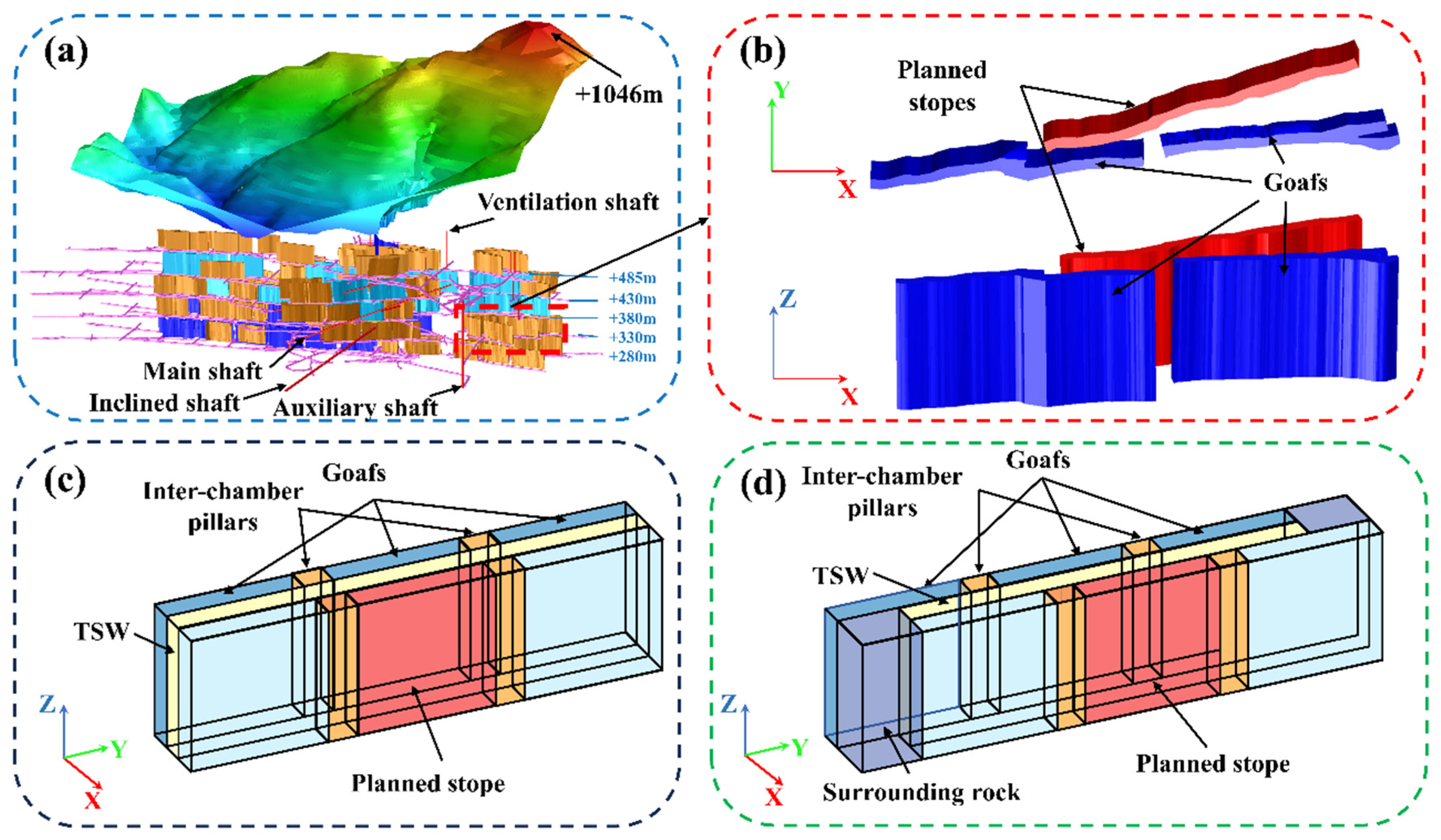
2.1. Background

The Jubankeng tungsten mine, located in Lianping County, Guangdong Province, China, is a major underground source of high-quality wolframite ore. The deposit comprises steeply dipping, thin to extremely thin ore bodies, including both single-vein and vein-belt types. Since commencing operations in the early 1980s, the mine has developed 12 levels ranging in depth from 280 m to 805 m.

The surrounding rock consists of metamorphic sandstone and hard rock types such as slate, brilliant porphyry, and gabbro. These rocks feature mostly wavy and flat-closed joints with relatively few horizontal joints. Some joints are filled with gravel, quartz, and mud. Overall, the rock mass is moist, with occasional water seepage. Figure 1a presents a comprehensive 3D model of the Jubankeng mine.

Currently, the mine uses a medium-deep hole sublevel drill and benching method for segmental ore extraction. Stopes are aligned with the ore veins and measure approximately 50 m in length and height. Sill pillars range from 2.5 to 3.0 m, inter-chamber pillars from 3.0 to 8.0 m, and crown pillars from 2.0 to 5.0 m. In the case of narrow-vein mining, such as for gold or tungsten, the stope width is small and the roof generally experiences no significant deformation or failure [18,19]. However, the temporary stope wall (TSW) is subjected to asymmetric, localized loads and has a large exposed area, making it particularly vulnerable to instability due to nearby goafs. Figure 1b shows a typical residual ore recovery project at the Jubankeng mine. Figure 1c illustrates a case where the planned stopes completely overlap with existing goafs, while Figure 1d shows a case where such overlap is only partial.

Hence, a key consideration in the recovery of residual resources is determining the optimal spatial relationship between planned stopes and goafs to ensure the structural stability of the recovery area.

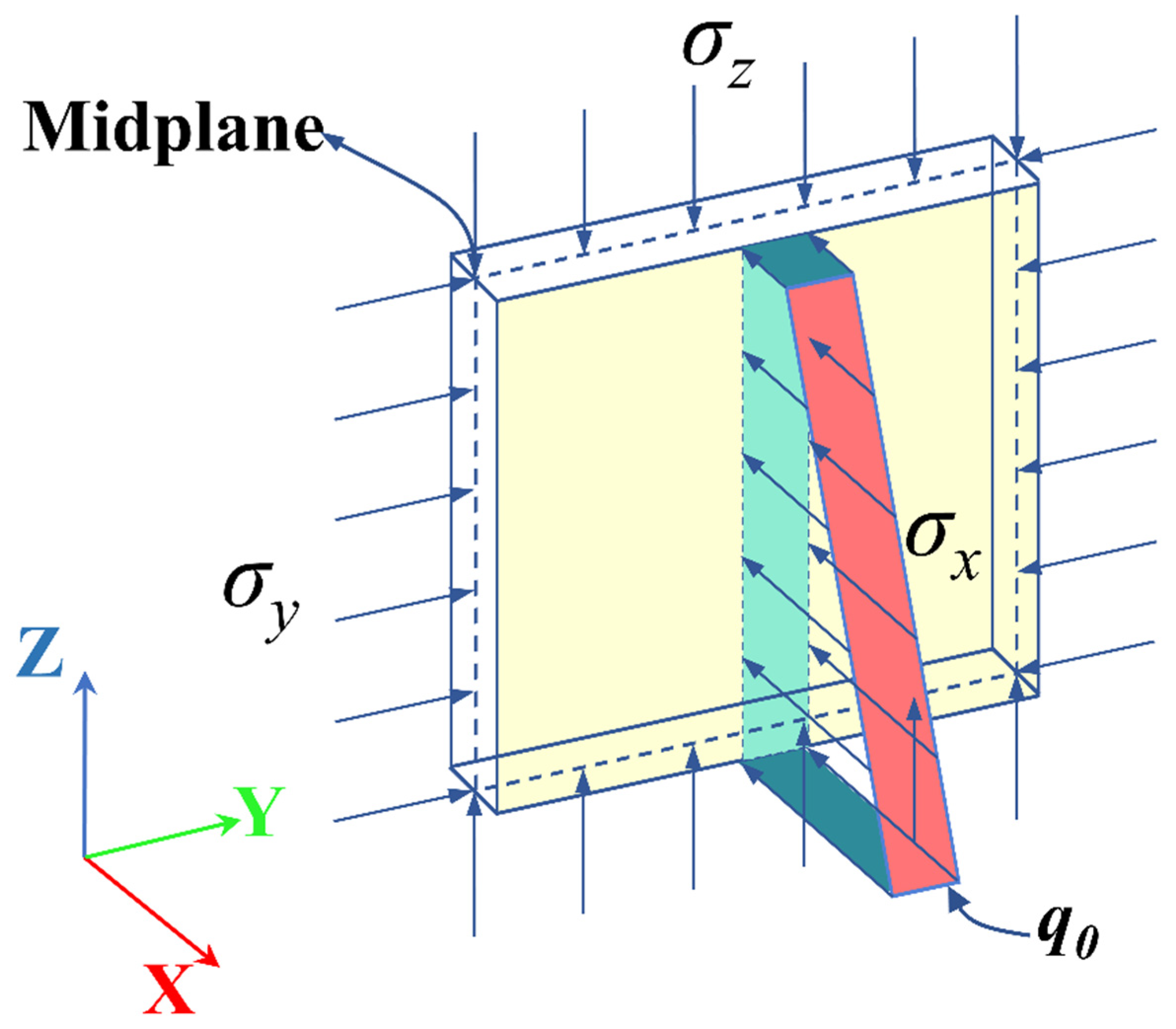
2.2. Mechanical Model

According to previous research [9,20,21,22,23], the ratio of a plate’s thickness to its minimum side length can be used to classify it as a thick plate (ratio > 1/5 to 1/8), a thin plate (ratio between 1/80 to 1/100 or 1/5 to 1/8), or a thin film (ratio < 1/80 to 1/100). For TSWs located between planned stopes and goafs, the classical small-deflection bending theory for thin plates is appropriate. This is because the surrounding rock is brittle and exhibits limited deformation prior to failure [24]. Typically, the TSW thickness is much less than 1/10 of its minimum lateral dimension, which aligns with the thin plate assumptions in elastic mechanics [25,26]. Therefore, thin plate theory can be used to analyze TSW stability. To simplify the analysis, the following assumptions are made:

(1)

The TSW is considered a continuous, homogeneous material after discounting the in situ rock strength.

(2)

The TSW surface is smooth and uniform in width, which is represented by the average actual width in the model. Dynamic disturbances from blasting are neglected.

(3)

Displacements induced by loading are small, and boundary displacements are minimal due to the relatively large TSW size.

(4)

Once plastic damage initiates, the load-bearing capacity of the TSW drops significantly, and even minor stress variations can result in large lateral deflections. This assumption is valid in hard rock mining environments.

(5)

There is negligible plastic deformation at the contact interfaces between the TSW and the surrounding rock, consistent with conditions in hard rock mines.

(6)

Stress analysis conforms to the standard sign conventions of elastic mechanics.

Based on in situ geostress test results from the mine, the central section of the +330 level exhibits a maximum principal stress ${\sigma }_{\mathrm{z}}$ oriented vertically, a middle principal stress ${\sigma }_x$ that is nearly horizontal and perpendicular to the ore body’s strike direction, and a minimum principal stress ${\sigma }_y$ that is nearly horizontal and aligned with the strike direction. Accordingly, this study adopts a lateral stress factor $\lambda =0.8$ to represent the in situ stress condition. Following the excavation of the planned stopes, stress redistribution occurs. Stress concentration and release are observed ${\sigma }_{\mathrm{z}}$ in the z-direction, while stress release also takes place ${\sigma }_y$ in the y-direction. In contrast, lateral stress ${\sigma }_x$ in the x-direction remains concentrated along the inter-chamber pillars between adjacent goafs.

Figure 2 shows the mechanical model of the TSW, where ${\sigma }_y$ and ${\sigma }_{\mathrm{z}}$ represent the longitudinal and transverse loads on the TSW, respectively. The lateral stresses at the retained position of the inter-chamber pillars are applied to the localized TSW surfaces with a maximum lateral load of q₀. Since both the upper/lower and left/right boundaries of the TSW are composed of metamorphic sandstone, all edges are considered fixed and supported—i.e., no displacement or rotation is allowed. This assumption simplifies the analysis to a rectangular thin plate under combined transverse and longitudinal loading, along with localized lateral loads.

The TSW is made of metamorphic sandstone, a hard–brittle rock that does not undergo significant deformation before failure. This suggests that the use of the mechanical model to compute the stress state of TSWs is consistent with the basic assumptions. Preliminary analysis of the mechanical model shows that the stress state of TSWs is primarily influenced by structural parameters and in situ stresses. Structural parameters, such as length, height, and thickness, play a key role, with thickness directly determining the bending stiffness of the TSW. When the thickness is smaller, the stresses are larger. Furthermore, as the in situ stress in the x-direction increases, the bending effects cause the stress state of the TSW to be more significantly influenced by the in situ stress. In conclusion, under fixed geological conditions, the stress state of TSWs is mainly determined by bending stiffness and the magnitude of the in situ stress in the x-direction. Future research will focus on the impact of these two factors on TSW stability.

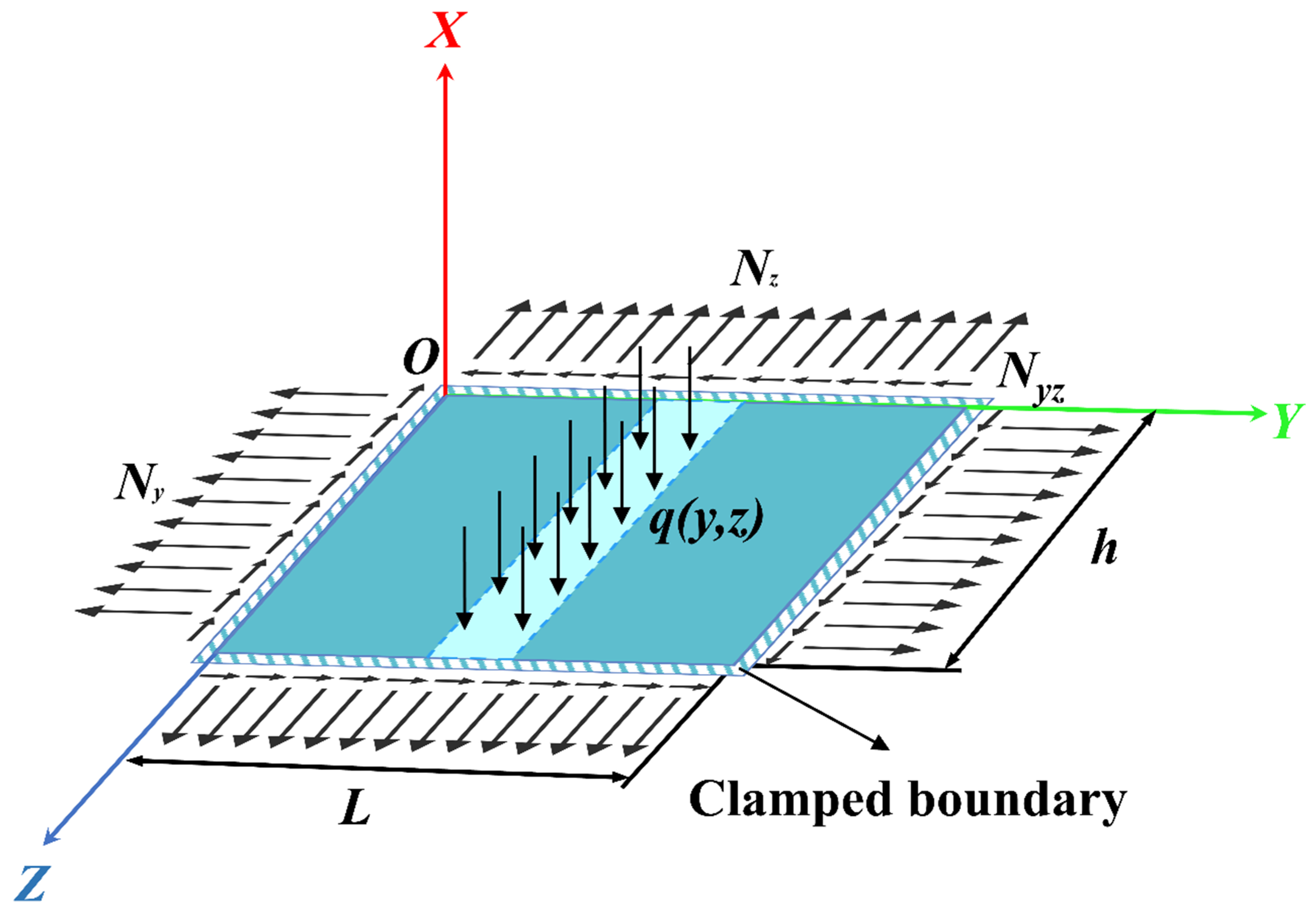
3. Analysis of Mechanical Model of Rectangular Plate Supported on Four Edges Under Local Lateral Load, Longitudinal and Transverse Load

3.1. Thin Plate Differential Equilibrium Equation

Figure 3 shows the force distribution on a rectangular thin plate with all four edges supported, subject to transverse loads, longitudinal loads, and in-plane localized lateral forces (including shear). This generalized model supports broader theoretical derivation beyond the specific conditions in Figure 2.

The purpose of using the general thin plate model for analysis and research is to make the theoretical derivation have a wider applicability; if the transverse and longitudinal loads are small, the bending effect for the thin plate can be ignored. In this case, the stress superposition effect brought by the longitudinal and transverse loads on the thin plate can be disregarded; however, when the longitudinal and transverse loads reach a certain level, the effect of the longitudinal and transverse loads on the bending effect of the thin plate must be considered. Due to the localized lateral force applied to the Z-Y plane, the value of which varies with different positions of the thin plate, it is expressed as a function with reference to y and z. Thus, the governing differential equation of the thin plate is as follows:

$$D{\nabla }^{4}w-\left(N_y{\displaystyle \frac{{\partial }^{2}w}{\partial y^2}}+N_z{\displaystyle \frac{{\partial }^{2}w}{\partial z^2}}+2N_{yz}{\displaystyle \frac{{\partial }^{2}w}{\partial y\partial z}}\right)=q\left(y,z\right)$$

(1)

$$D=E{W}_b^3/12\left(1-{\mu }^2\right)$$

(2)

where D is the flexural rigidity, $w$ is the deflection, E is Young’s modulus, $\mu$ is Poisson’s ratio, $W_b$ is the thickness of the thin plate, $N_y$, $N_{\mathrm{z}}$, $N_{\mathrm{yz}}$ are in-plane forces per unit width along the edge of the thin plate ($N_{\mathrm{yz}}$ is the in-plane shear force, and $N_y$ and $N_{\mathrm{z}}$ are normal forces), $q\left(y,z\right)$ is the localized lateral force on the plate per unit area.

Because the in-plane shear forces $N_{\mathrm{yz}}$ at the boundaries of the thin plate are zero [17], the influence of in-plane shear forces on the bending behavior of the thin plate can be ignored; so, the formula (1) can be simplified as follows:

$$D{\nabla }^{4}w-\left(N_y{\displaystyle \frac{{\partial }^{2}w}{\partial y^2}}+N_z{\displaystyle \frac{{\partial }^{2}w}{\partial z^2}}\right)=q(y,z)$$

(3)

$$q(y,z)={\displaystyle \sum _{m=1}^{\infty }{\displaystyle \sum _{n=1}^{\infty }{q}_{mn}}}\sin {\displaystyle \frac{m\pi y}{L}}\sin {\displaystyle \frac{n\pi z}{h}}$$

(4)

For linear loads localized laterally and varying with the z-direction, the Fourier coefficients $q_{mn}$ in Formula (3) are determined based on Formula (a) on page 111 of Theory of plates and shells [23]. Consequently, the Fourier coefficients $q_{mn}$ in Formula (3) are calculated as follows:

$$q_{mn}={\displaystyle \frac{4q}{Lh}}{\displaystyle {\int }_{y_0-a/2}^{y_0+a/2}{\displaystyle {\int }_{z_0-h/2}^{z_0+h/2}\sin \frac{m\pi y}{L}}}\sin {\displaystyle \frac{n\pi z}{h}}dydz$$

(5)

$$q=q_0-kz$$

(6)

where $q$ is the linear load, $L$ is the stope length, $h$ is the stope height, $\left(y_0,z_0\right)$ is coordinates of the localized lateral load center, a is width of inter-chamber pillar, $q_0$ is maximum value of lateral load in thin plate, k is lateral load per unit.

3.2. Determining Coefficients for Deflection Expressions with Additional Terms

The governing equation above is a non-homogeneous partial differential equation in terms of deflection. While a closed-form integration method exists, it becomes complex when accounting for the effects of both transverse and longitudinal loads [27,28]. Hence, the superposition method is commonly used for thin plates with all edges supported [23,29]. To further simplify the solution, the method of complementary terms can be applied. Yan [30] introduced a deflection expression that includes supplementary terms, offering both ease of calculation and broad applicability. The general deflection expression is given as follows:

$$\omega ={\displaystyle \sum _{m=1}^{\infty }{\displaystyle \sum _{n=1}^{\infty }{b}_{mn}}}\sin {\displaystyle \frac{m\pi y}{L}}\sin {\displaystyle \frac{n\pi z}{h}}+{\displaystyle \sum _{n=1}^{\infty }{F}_n\left(y\right)}\sin {\displaystyle \frac{n\pi z}{h}}+{\displaystyle \sum _{m=1}^{\infty }{F}_m\left(z\right)}\sin {\displaystyle \frac{m\pi y}{L}}$$

(7)

where

$$F_n\left(y\right)={\displaystyle \frac{1}{6L}}\left({\displaystyle \frac{A_{\mathrm{n}}-B_{\mathrm{n}}}{D}}\right)y^3-{\displaystyle \frac{1}{2}}{\displaystyle \frac{A_n}{D}}{y}^2+{\displaystyle \frac{L}{6D}}\left(A_{\mathrm{n}}+2B_n\right)y$$

(8)

$$F_m\left(z\right)={\displaystyle \frac{1}{6h}}\left[{\displaystyle \frac{C_m-D_{\mathrm{m}}}{D}}\right]z^3-{\displaystyle \frac{1}{2}}{\displaystyle \frac{C_m}{D}}{z}^2+{\displaystyle \frac{h}{6D}}\left(C_m+2D_m\right)z$$

(9)

In Formula (7), the term $b_{mn}$ represents the Fourier coefficient of the deflection expression. According to the derivation results from the book Fourier Series Solutions in Structural Mechanics [30], the deflection coefficient $b_{mn}$ as follows:

$$b_{mn}={\displaystyle \frac{g_n+g_m+\frac{q_{mn}}{D}}{\left[{({\alpha }_{\mathrm{m}}^2+{\beta }_n^2)}^2+{\alpha }_{\mathrm{m}}^2\frac{N_{\mathrm{y}}}{D}+{\beta }_n^2\frac{N_z}{D}\right]}}$$

(10)

$$g_n=-{\displaystyle \frac{2}{m\pi D}}\left[{\beta }_n^2\left(2+{\displaystyle \frac{{\beta }_n^2}{{\alpha }_{\mathrm{m}}^2}}\right)+{\displaystyle \frac{N_y}{D}}+{\displaystyle \frac{{\beta }_n^2}{{\alpha }_{\mathrm{m}}^2}}{\displaystyle \frac{N_z}{D}}\right]\left[A_{\mathrm{n}}+(-1{)}^{\mathrm{m}+1}{B}_{\mathrm{n}}\right]$$

(11)

$$g_m=-{\displaystyle \frac{2}{\mathrm{n}\pi D}}\left[{\alpha }_{\mathrm{m}}^2\left(2+{\displaystyle \frac{{\alpha }_{\mathrm{m}}^2}{{\beta }_n^2}}\right)+{\displaystyle \frac{{\alpha }_{\mathrm{m}}^2}{{\beta }_n^2}}{\displaystyle \frac{N_{\mathrm{y}}}{D}}+{\displaystyle \frac{N_z}{D}}\right]\left[C_m+(-1{)}^{\mathrm{n}+1}{D}_{\mathrm{m}}\right]$$

(12)

where ${\alpha }_m={\displaystyle \frac{m\pi }{L}}$, ${\beta }_n={\displaystyle \frac{n\pi }{h}}$.

The coefficients $A_{\mathrm{n}}$, $B_{\mathrm{n}}$, $C_m$, $D_{\mathrm{m}}$ in Formulas (7) to (12) represent the sinusoidal steps of the normal bending moments on the left edge ((y = 0), as shown in Figure 3), the right edge (y = L), the back edge (z = 0), and the front edge (z = h) of the rectangular thin plate. The expression for the sinusoidal steps of the normal bending moments on these four edges is as follows:

$$\left\{\begin{array}{l}{M}_y(0,z)={\displaystyle \sum _{n=1}^{\infty }{A}_n}\sin {\displaystyle \frac{n\pi z}{h}}\hfill \\ M_y(L,z)={\displaystyle \sum _{n=1}^{\infty }{B}_n}\sin {\displaystyle \frac{\mathrm{n}\pi z}{h}}\hfill \\ M_z(y,0)={\displaystyle \sum _{m=1}^{\infty }{C}_m}\sin {\displaystyle \frac{m\pi y}{L}}\hfill \\ M_z(y,h)={\displaystyle \sum _{m=1}^{\infty }{D}_m}\sin {\displaystyle \frac{m\pi y}{L}}\hfill \end{array}\right.$$

(13)

The coefficients $A_{\mathrm{n}}$, $B_{\mathrm{n}}$, $C_m$, $D_{\mathrm{m}}$ in Formulas (8) to (12) need to be determined based on the boundary supported conditions of the rectangular thin plate. These coefficients $A_{\mathrm{n}}$, $B_{\mathrm{n}}$, $C_m$, $D_{\mathrm{m}}$ represent the sine function of the normal moments on the edges as outlined in Formula (13). This paper explores a rectangular thin plate fixed and supported on all four edges; Thus, the values of these coefficients $A_{\mathrm{n}}$, $B_{\mathrm{n}}$, $C_m$, $D_{\mathrm{m}}$ must be determined through the boundary conditions of the edges.

The four edges of the TSW are all connected to the original rock, and their boundary displacements are basically negligible and boundaries are fixed and supported by the surrounding rock, similar to a thin plate with four fixed and supported edges, The deflection and angular displacement around the perimeter of the rectangular thin plate are zero. Thus, TSW’s boundary conditions are expressed as follows:

$$\begin{array}{c}{\left.w\right|}_{z=0,h}=0,{\left.{\displaystyle \frac{\partial w}{\partial z}}\right|}_{z=0,h}=0\\ {\left.w\right|}_{y=0,L}=0,{\left.{\displaystyle \frac{\partial w}{\partial y}}\right|}_{y=0,L}=0\end{array}$$

(14)

Consider the left edge of the rectangular thin plate. The boundary’s condition on this edge is both fixed and supported, resulting in an angular displacement of zero at (y = 0). This implies that the partial derivative of deflection $w$ with respect to y must also be zero at this boundary:

$${\left.{\displaystyle \frac{\partial \omega }{\partial y}}\right|}_{y=0}={\displaystyle \sum _{m=1}^{\infty }{\displaystyle \sum _{n=1}^{\infty }\frac{m\pi }{L}{b}_{mn}\sin \frac{n\pi z}{h}+{\displaystyle \sum _{n=1}^{\infty }\left[\frac{L}{6D}(2A_n+B_n)\right]\sin \frac{n\pi z}{h}+{\displaystyle \sum _{m=1}^{\infty }\frac{m\pi }{DL}}}{F}_m\left(z\right)}}$$

(15)

By expanding z, z², and z³ into a sinusoidal series, Formula (15) can be simplified to:

$${\left.{\displaystyle \frac{\partial \omega }{\partial y}}\right|}_{y=0}={\displaystyle \sum _{n=1}^{\infty }\left[{\displaystyle \sum _{m=1}^{\infty }\frac{m\pi }{L}{b}_{mn}+\frac{L}{6D}(2A_n+B_n)+\frac{2h^2}{D{\pi }^3{n}^3}{\displaystyle \sum _{m=1}^{\infty }\left(C_m+{(-1)}^{n+1}{D}_m\right)}}\frac{m\pi }{L}\right]}\sin {\displaystyle \frac{n\pi y}{h}}$$

(16)

The left edge of the rectangular thin plate (y = 0) is a fixed and supported edge with zero angular displacement. By setting Formula (16) equal to zero, the following equation is obtained:

$${\displaystyle \frac{\pi }{a}}{\displaystyle \sum _{m=1}^{\infty }m{b}_{mn}+\frac{L}{6D}(2A_n+B_n)+\frac{2h^2}{D{\pi }^2{n}^{3}L}{\displaystyle \sum _{m=1}^{\infty }m\left(C_m+{(-1)}^{n+1}{D}_m\right)}}=0$$

(17)

Similarly, the equations for the remaining three edges concerning the coefficients $B_{\mathrm{n}}$, $C_m$, and $D_{\mathrm{m}}$, to be determined, respectively.

3.3. Calculation of Bending Moments, and Internal Forces in Thin Plates

Based on the formula in Theory of Plates and Shells [23], the bending moment in the cross-section of a rectangular thin plate can be calculated as follows:

$$\left\{\begin{array}{l}{M}_y=-D\left({\displaystyle \frac{{\partial }^{2}w}{\partial y^2}}+\mu {\displaystyle \frac{{\partial }^{2}w}{\partial z^2}}\right)\\ M_z=-D\left({\displaystyle \frac{{\partial }^{2}w}{\partial z^2}}+\mu {\displaystyle \frac{{\partial }^{2}w}{\partial y^2}}\right)\\ M_{yz}=-D\left(1-\mu \right){\displaystyle \frac{{\partial }^{2}w}{\partial y\partial z}}\end{array}\right.$$

(18)

In the thickness direction of the TSW, the maximum stress component occurs at the mid-thickness interface ($x={\displaystyle \frac{W_b}{2}}$). Therefore, the maximum stress at each point along the TSW can be determined as follows:

$$\left\{\begin{array}{l}{\sigma }_y={\displaystyle \frac{6M_y}{W_{\mathrm{b}}^2}}\\ {\sigma }_z={\displaystyle \frac{6M_z}{W_{\mathrm{b}}^2}}\\ {\tau }_{yz}={\displaystyle \frac{12M_{yz}}{W_{\mathrm{b}}^2}}\end{array}\right.$$

(19)

Because the internal forces in the thin plate calculated using this method are per unit length, the length of the edge of the TSW in the corresponding direction must be divided to determine the stresses applied within the TSW. The effect of ${\sigma }_x$ in the thin plate can be neglected. According to the basic theory of plane stress problems, the ultimate positive stress at each point within the TSW can be calculated by the following equation:

$$\left\{\begin{array}{c}{\sigma }_{\max }={\displaystyle \frac{{\sigma }_y+{\sigma }_z}{2}}+\sqrt{{\left({\displaystyle \frac{{\sigma }_y-{\sigma }_z}{2}}\right)}^2+{\tau }_{yz}^2}\\ {\sigma }_{\min }={\displaystyle \frac{{\sigma }_y+{\sigma }_z}{2}}-\sqrt{{\left({\displaystyle \frac{{\sigma }_y-{\sigma }_z}{2}}\right)}^2+{\tau }_{yz}^2}\end{array}\right.$$

(20)

From the analysis of the mechanical model above, it can be seen that at the midpoint of the left and right boundaries and the midpoint of the lateral load on the top and bottom boundaries, the TSW experiences the ${\sigma }_{\max }$ and ${\sigma }_{\min }$ on both sides. This indicates that the failure of the TSW begins at these midpoint locations, both at the boundary and lateral load center.

3.4. TSWs Yield Judgment Method

When the rock material is subjected to tensile-shear action under the influence of a secondary stress field, the Drucker–Prager yield criterion can be utilized to determine the yield state of TSWs. The yield strength of TSWs under different stress states can be calculated using the following equation:

$$f=\sqrt{J_2}+\alpha I_1-K=0$$

(21)

where $J_2$ is the second deviatoric invariant and $J_2={\displaystyle \frac{1}{2}}(S_{ij}{S}_{ij})={\displaystyle \frac{1}{2}}\left[{\left({\sigma }_y-{\sigma }_z\right)}^2+{\sigma }_y^2+{\sigma }_z^2+6{\tau }_{yz}^2\right]$, $S_{ij}$ is the deviatoric stress tensor, $I_1={\sigma }_y+{\sigma }_z$ is the first stress invariant, $\alpha$ and K are the material constants given by:

$$\alpha ={\displaystyle \frac{2\sin \phi }{\sqrt{3}(3+\sin \phi )}}$$

(22)

$$K={\displaystyle \frac{6C\cos \phi }{\sqrt{3}(3+\sin \phi )}}$$

(23)

where C and $\phi$ are the cohesion and internal friction angle of rock mass, respectively.

4. Calculation and Analysis of Mechanical Models

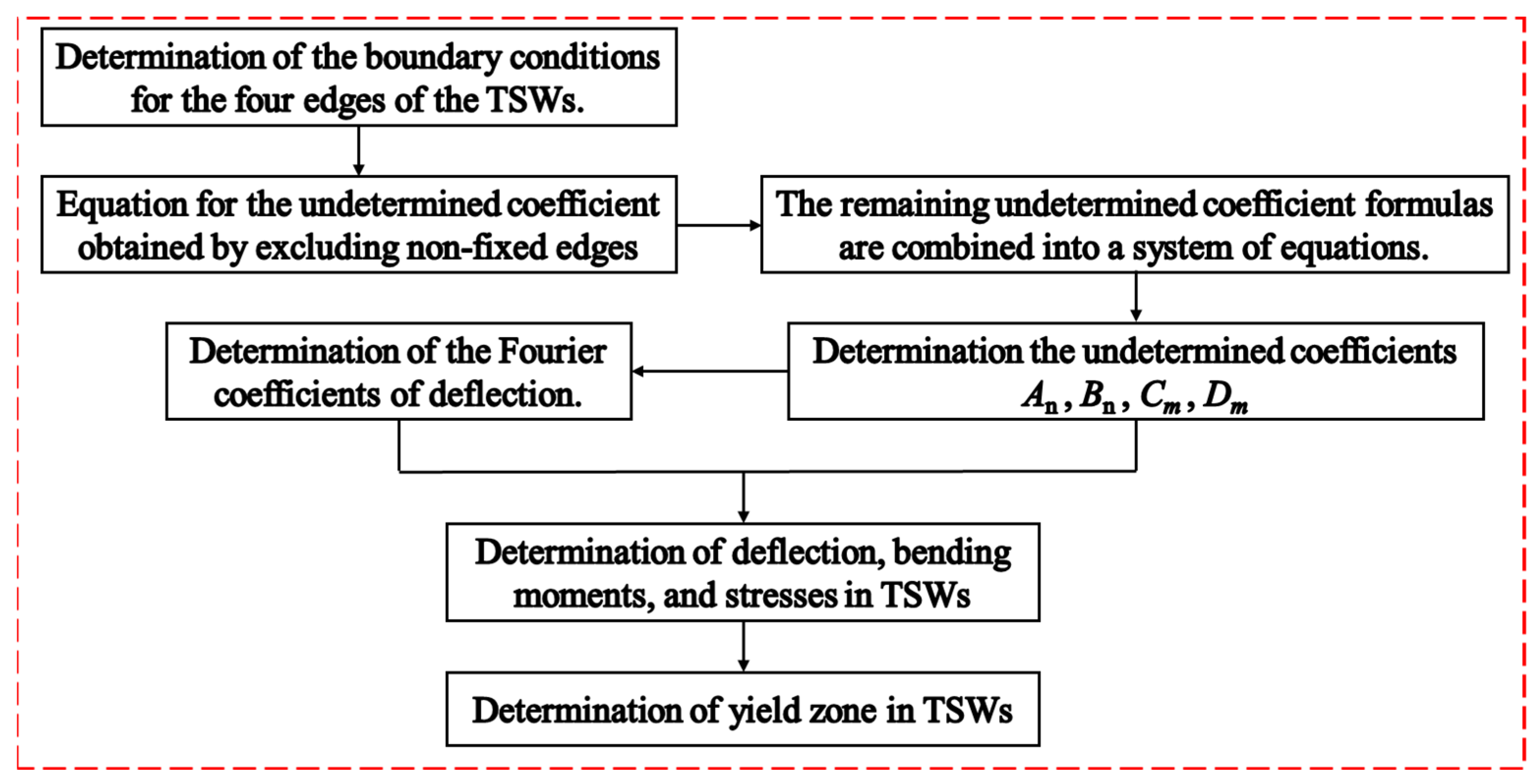
4.1. Calculation Procedure

Based on the analysis of the deflection and bending moment calculation method for a rectangular plate supported on all four edges, the steps for calculating the deflection and bending moment of the TSW using this method are shown in Figure 4.

First, because all four sides of the TSW have fixed and supported edges, Formula (17) is combined into a system of equations to calculate the undetermined coefficients $A_{\mathrm{n}}$, $B_{\mathrm{n}}$, $C_m$, and $D_{\mathrm{m}}$.

After calculating the undetermined coefficients, the Fourier coefficients of deflection are computed using Formulas (10) to (12).

Next, deflection is calculated using Formulas (7) to (9), bending moments are determined using Formula (18), and the maximum and minimum principal stresses are computed using Formula (20).

Finally, the yield state of TSWs is determined using Formulas (21) to (23).

In subsequent calculations, the system of linear equations is solved using the sparse matrix decomposition method. The program is written in C++ and uses double precision for real variables.

4.2. Determining Calculation Parameters

Many years of mining have resulted in goafs forming in the middle section at a depth of +330 m (h₀ = 547 m). To recover the residual ore resources, the mine plans to use the medium-deep hole sublevel drilling and benching method to extract ore from the veins surrounding the goafs. The initial stress of TSWs after mining in the planned stopes can typically be calculated using the tributary area method [31] with the following equation:

$${\sigma }_z^{\prime }=\gamma h_0\left(1+{\displaystyle \frac{W_b}{B}}\right)$$

(24)

$${\sigma }_x^{\prime }={\sigma }_y^{\prime }=\lambda {\sigma }_z^{\prime }$$

(25)

where $\lambda$ is the lateral stress factor, $\gamma$ is the rock capacity.

As shown in Figure 2, the in-plane forces per unit length in the y-direction and z-direction are as follows:

$$N_y=-W_b{\sigma }_y^{\prime }$$

(26)

$$N_z=-W_b{\sigma }_z^{\prime }$$

(27)

The relevant parameters needed for calculating the theoretical approach are presented in

Table 1. Relevant parameters of the mine.

Parameters	Value	Units
Stope length (L)	50	m
Stope width (B)	4	m
Stope height (h)	50	m
Sidewall thickness (Wb)	3	m
Inter-chamber pillar width (a)	4	m
In-plane force in the y-direction (Ny)	47.2	MN·m−1
In-plane force in the z-direction (Nz)	78.8	MN·m−1
maximum value of lateral load (q0)	22.1	MPa
lateral load per unit (k)	0.044	MPa·m−1

.

The Hoek–Brown strength criterion, a widely used method for evaluating the strength of hard rock masses [32], was employed to determine the rock mechanical parameters. The mechanical properties of the surrounding rock and ore body in the mine are presented in

Table 2. Physical and mechanical parameters of the rocks.

Rock Type	Orebody	Surrounding Rock	Units
Density	2800	2500	kg·m−3
Elastic modulus	32.5	20.0	GPa
Cohesion	5.2	4.9	MPa
Internal friction angle	50.0	36.0	°
Tensile strength	5.0	4.6	MPa
Poisson ratio	0.26	0.3	N/A

.

4.3. Determining the Number of Convergent Series Terms in the Mechanical Model

The calculation parameters from the previous section are used, with all four edges of the TSWs under fixed and supported conditions. The number of graded terms for the calculation is set to 5, 10, 20, 30, 40, 50, 60, 70, and 80, respectively.

According to Theory of Plates and Shells [23], the deflection of the thin plate is $w=w_{mn}{\displaystyle \frac{q{L}^4}{D}}$ and its bending moments is $M=M_{mn}q{L}^2$. By analyzing the changes in dimensionless quantities such as deflection coefficient ${\displaystyle \frac{D·w\left(L/2,h/2\right)}{q{L}^4}}$ at the center of the thin plate, the bending moment coefficient ${\displaystyle \frac{M_y\left(L/2,h/2\right)}{q{L}^2}}$ in the y-direction at the center of the thin plate, the bending moment and coefficient ${\displaystyle \frac{M_y\left(0,h/2\right)}{q{L}^2}}$ in the y-direction at the left midpoint of the thin plate, the number of convergent level terms of the mechanical model can be determined. The calculation results are shown in

Table 3. Computed results by different number of series terms.

Number of Term in Series	${\mathit{w}}_{\mathit{m}\mathit{n}}$ (L/2,h/2)	${\mathit{M}}_{\mathit{y}\mathit{m}\mathit{n}}$ (L/2,h/2)	${\mathit{M}}_{\mathit{y}\mathit{m}\mathit{n}}$ (0,h/2)
5	0.00016991734	0.003578805	−0.001246028
10	0.00016982046	0.003574659	−0.001247692
20	0.00016976138	0.003537642	−0.001247242
30	0.00016973226	0.003562551	−0.001247599
40	0.00016972079	0.003550222	−0.001247482
50	0.00016971889	0.003552966	−0.001247585
60	0.00016971786	0.003551420	−0.001247520
70	0.00016971715	0.003553237	−0.001247567
80	0.00016971682	0.003552425	−0.001247539

.

As seen in the calculation results in Table 3, once the number of gradation terms reaches 20, the first three significant figures of the deflection coefficient at the center of the thin plate remain unchanged. After 40 terms, the first four significant figures of the deflection coefficient at the center of the thin plate stabilize, as do the first three significant figures of the y-direction moment coefficient at the center of the thin plate. Additionally, the first four significant figures of the y-direction moment coefficient at the left edge of the thin plate remain consistent. Thus, it can be concluded that with 40 gradation terms, convergence has been achieved, and subsequent calculations in this paper will use the results based on 40 gradation terms.

4.4. Comparative Study of Computational Results with Existing Method

Two commonly used thin plate mechanical models are available: one is the Theory of Plates and Shells model [23], which calculates deflection and bending moment under fixed boundary conditions and uniform distributed load; the other is the theoretical model from the Handbook of Building Structural Statics [33], which calculates the bending moment under simple support boundary conditions. To compare these two commonly used methods with the results from this study, TSW structural parameters are taken from Section 4.2. The in-plane forces in the y- and z-directions are assumed to be in situ stresses, while the load in the x-direction is a uniformly distributed load over the entire TSW side. The deflection and bending moment coefficients calculated by the different models are shown in

Table 4. Comparison with the results calculated by the two theoretical methods.

Calculation Method	${\mathit{w}}_{\mathit{m}\mathit{n}}$ (L/2,h/2)	${\mathit{M}}_{\mathit{y}\mathit{m}\mathit{n}}$ (L/2,h/2)	${\mathit{M}}_{\mathit{z}\mathit{m}\mathit{n}}$ (L/2,h/2)	${\mathit{M}}_{\mathit{y}\mathit{m}\mathit{n}}$ (0,h/2)
This paper	0.0013246	0.024199	0.024209	−0.052965
Theory of Plates and Shells	0.00126	0.0231	0.0231	−0.0513
Error (%)	+4.88%	+4.54%	+4.58%	−3.14%
Working Group of Handbook of Building Structural Statics	-	0.0368	0.0368	-
Error (%)	-	−52.07%	−52.01%	-

.

According to Table 4, the results from the Theory of Plates and Shells show an error of less than 5% compared to the results from this study, while the error between the results from the Working Group of the Handbook of Building Structural Statics and this study is 52%. This demonstrates that the results from this study more effectively account for the influence of in situ stresses and boundary conditions.

It is noteworthy that when boundary stresses are not considered, the results from this study match those obtained from the Theory of Plates and Shells. When boundary stresses are not considered and simple support conditions are applied, the results from this study align with those from the Working Group of the Handbook of Building Structural Statics. This indicates that the results from this study are consistent with previous models under certain conditions.

5. Stability Analysis of TSWs

5.1. Stress Distribution and Yield Zone Analysis of TSWs

Under large localized lateral loads, as well as transverse and longitudinal loads, significant bending stresses are induced in the thin sidewalls (TSWs), resulting in elevated maximum principal stresses (MPS) on both sides of the structure [34], which may compromise stability. As derived in Section III, the MPS and corresponding yield zones in the TSWs are primarily influenced by the lateral load center position (LP) and the spatial coordinates of the TSW.

Furthermore, because the host rock contains pre-existing joints and cracks and is affected by processes such as blasting, weathering, and hydraulic penetration [35,36,37,38], the rock’s cohesion should be reduced by a safety factor (SF). The yield behavior of the rock mass is assessed using the allowable cohesion, which incorporates this safety factor [9]. When the actual SF is lower than the allowable value, the rock enters a yield state; conversely, when the SF exceeds the allowable value, the rock remains relatively stable. In mining practice, a typical SF exceeds 1.25 to ensure safety; in this study, a value of 1.5 is adopted.

To analyze the MPS distribution and yield zones, a case study was conducted based on the actual conditions at the Jubankeng Tungsten Mine. The average TSW dimensions were set to 50 m (length) × 50 m (height) × 3 m (thickness), with a lateral load width (LW) of 4 m. The MPS and yield zone distributions were evaluated for LP values of 5 m, 10 m, 15 m, 20 m, and 25 m. The corresponding cloud diagrams of stress and yield zones are shown in Figure 5 and Figure 6.

As shown in Figure 5, when the LP is small, the zone of elevated MPS is concentrated near the left boundary of the TSW. As the LP increases, stress concentrations develop at the upper and lower boundaries and the lateral load center zone, while stresses at the left boundary gradually decrease. Eventually, the MPS at the upper/lower boundaries and center zone surpass those at the left boundary. This indicates that peak stress points tend to occur at the midpoint of the left boundary (0, h/2), at the lower boundary’s lateral load center (LP, 0), and at (LP, h/2). Additionally, the stress distribution becomes more uniform with increasing LP.

As shown in Figure 6, for smaller LP values, the yield zone appears primarily at the left boundary. With increasing LP, yield zones begin to appear at the upper and lower side boundaries, while the yield zone at the left boundary diminishes. Eventually, yield zones also emerge near the right boundary. Overall, yield zones become more evenly distributed across the TSW, indicating a gradual decrease in structural stability.

5.2. Analysis of Influencing Factors

Based on the analysis of the mechanical model in Section 3, it can be seen that the stress distribution of the TSW is influenced by factors such as the position of the lateral load center, lateral load width, TSW structural parameters, in situ stress magnitude and direction, and rock mechanical properties. In the Jubankeng tungsten mine residual ore recovery project, the mining depth and rock properties are fixed; so, the magnitude of in situ stresses and rock mechanical parameters remain constant. Therefore, this study primarily focuses on analyzing the impact of variables such as lateral load position (LP), lateral load width (LW), sidewall thickness (ST), sidewall length (SL), and sidewall height (SH) on the TSW stress distribution, further determining the MPS and yield zone distribution under different conditions. The parameters required for the mechanical model calculations are all derived from Section 4.2.

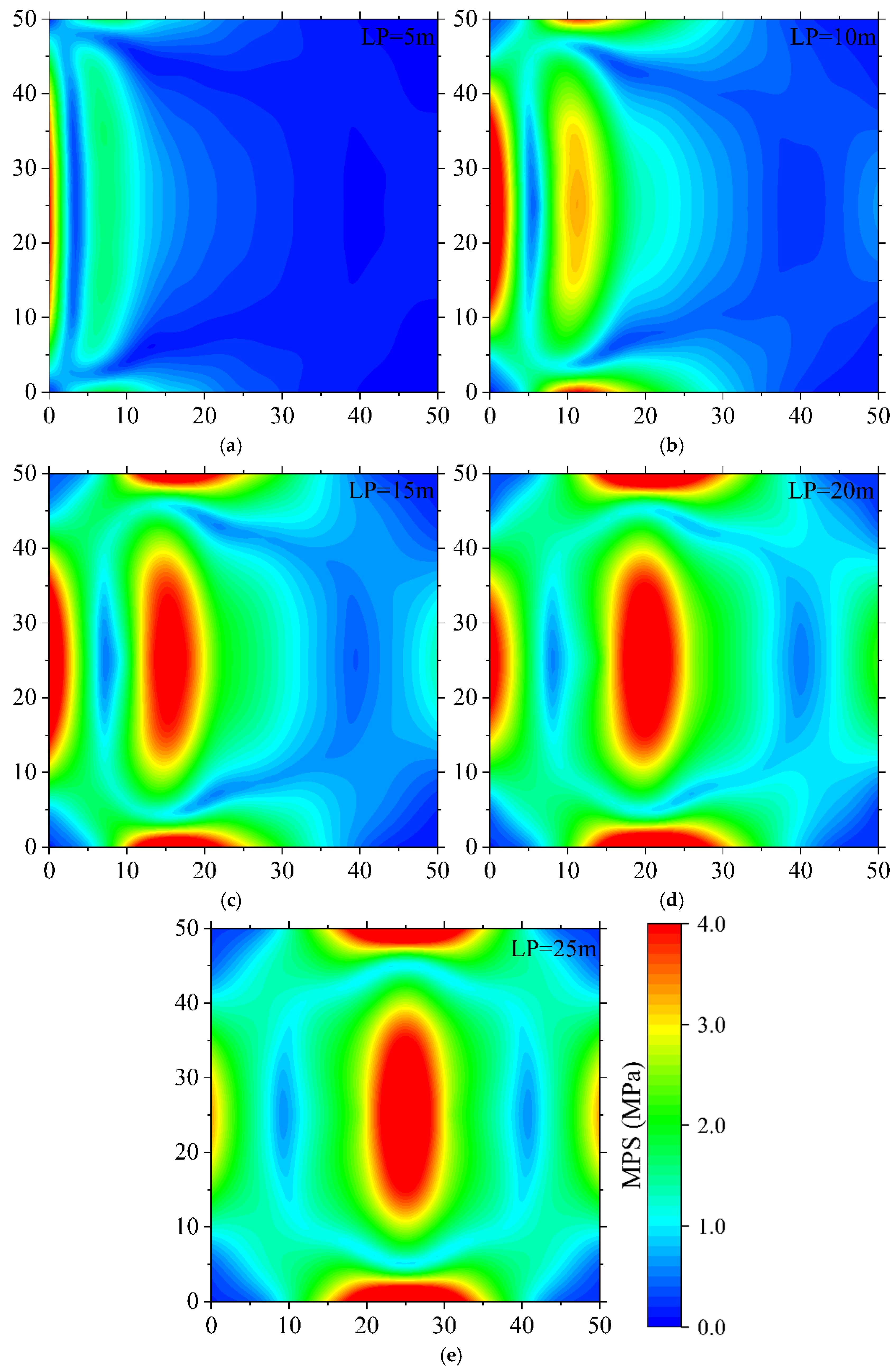
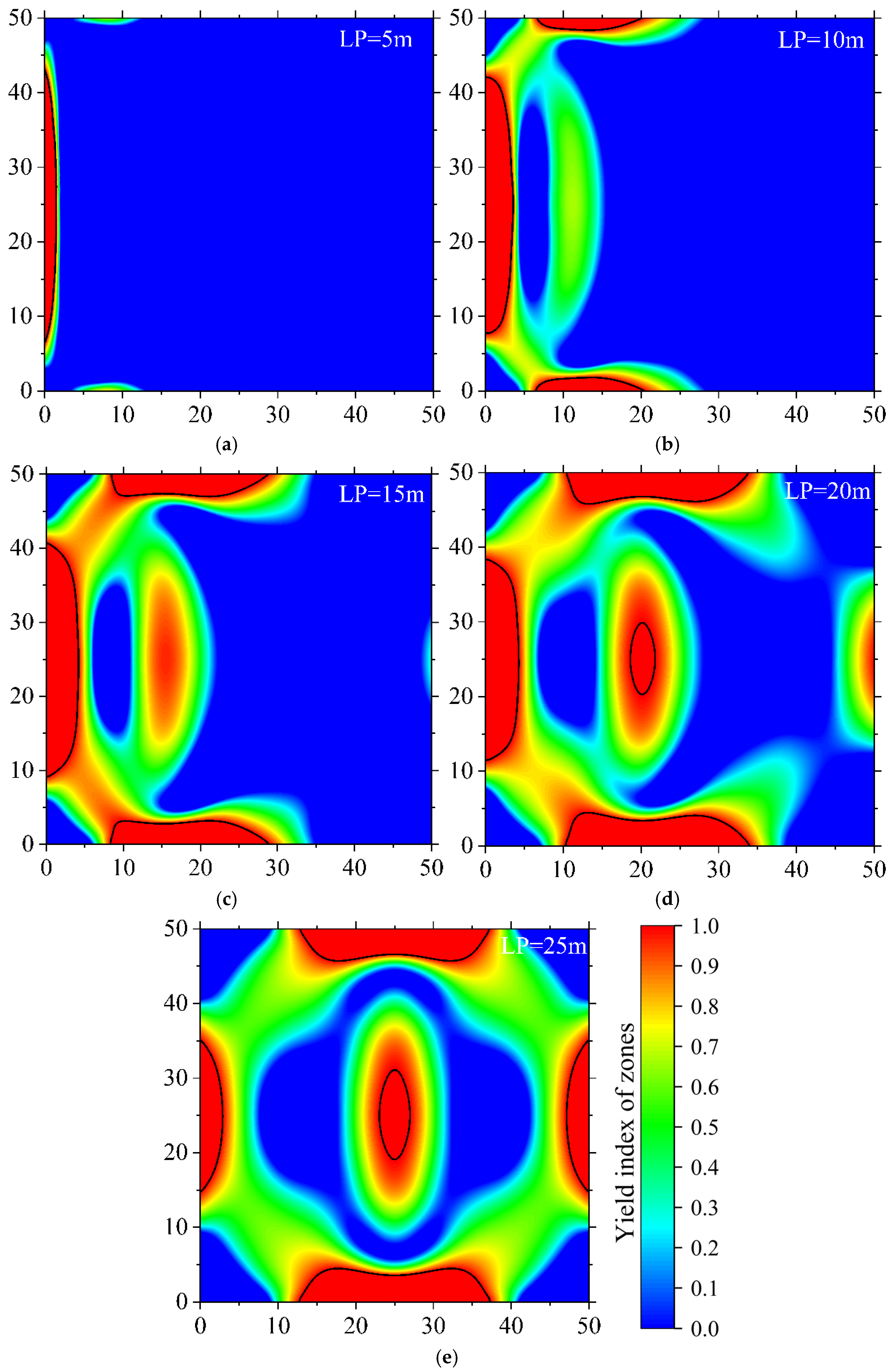
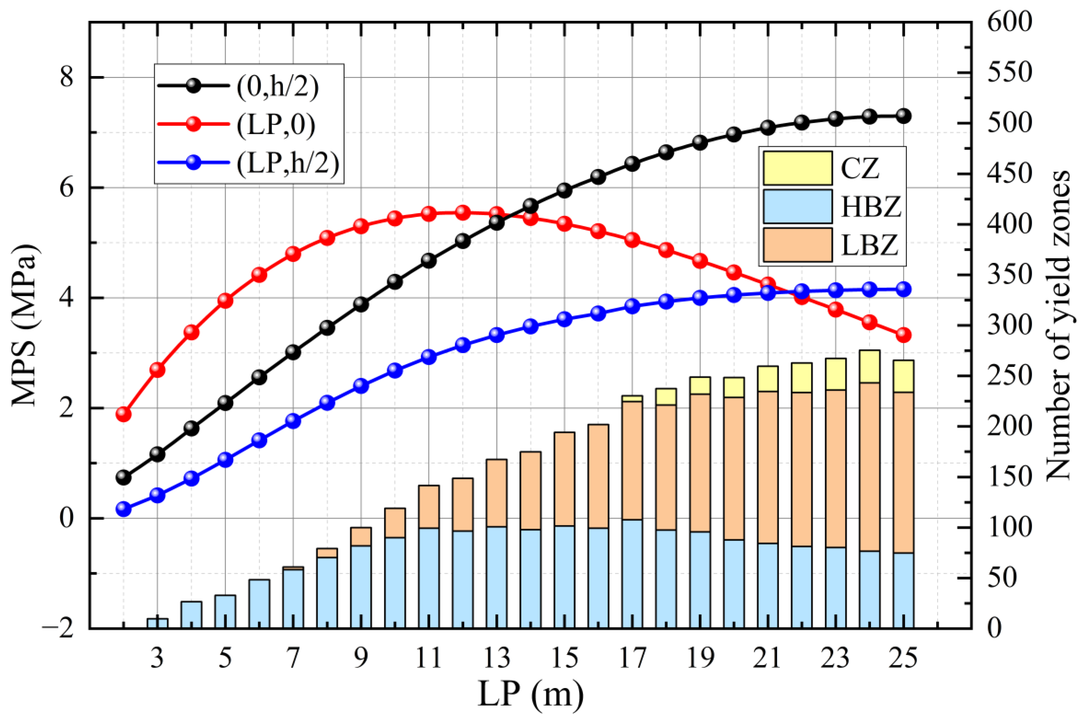
5.2.1. Influence of Lateral Load Center Position on TSW Stability

To investigate the influence of LP on TSW stability, the average TSW size was set to 50 m × 50 m × 3 m with a fixed LW of 4 m. MPS and yield zone data were computed for LP values ranging from 2 m to 25 m. Yield zones were categorized into three areas for statistical analysis: the height bounding zone (HBZ), the length bounding zone (LBZ), and the center zone (CZ). The variation in MPS and yield zones under different LPs is shown in Figure 7.

As the LP increases, the MPS at points (0, h/2) and (LP, h/2) first increase rapidly and then stabilize. The MPS at point (LP, 0) initially increases and later decreases, with a more pronounced rise than fall. When LP > 13 m, MPS at (0, h/2) exceeds that at (LP, 0); when LP ≥ 22 m, MPS at (LP, h/2) also exceeds (LP, 0). The yield zones in the HBZ increase and then decrease, while those in the LBZ start forming at LP ≥ 7 m and continue increasing. CZ yield zones begin forming at LP ≥ 17 m, with a decreasing rate of growth. The total yield zone count increases with the LP, with the rate slowing over time. When LP ≥ 17 m, both boundary and center zones are in a yield state.

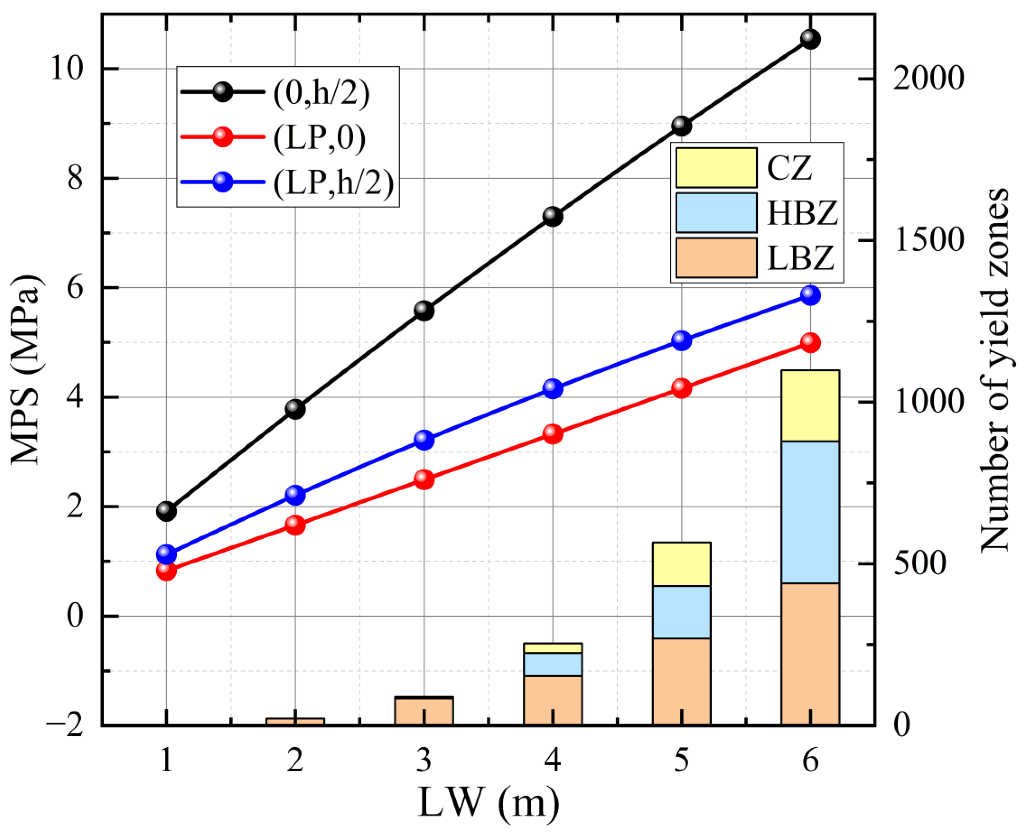
5.2.2. Influence of Lateral Load Width on TSW Stability

The effect of LW on stability was studied using the same TSW dimensions and LP set to 25 m. The LW values ranged from 1 m to 6 m. The variation in MPS and yield zones is shown in Figure 8.

MPS increases linearly with LW at all key points for a fixed LP and geometry. The increase rate is highest at (0, h/2), and similar at (LP, 0) and (LP, h/2). With increasing LW, yield zones in all areas increase continuously, reflecting reduced stability.

5.2.3. Influence of Sidewall Length and Height on TSW Stability

To study the relationship between SL, SH, and TSW stability, the MPS and the number of different yield zones for the weaker TSWs were calculated. For an SH of 20.0 m, 40.0 m, 60.0 m, 80.0 m, and 100 m, the average ST was set to 3 m, the SL to 50 m, the LP to 25 m, and the LW to 4 m. Additionally, for an SL of 20.0 m, 40.0 m, 60.0 m, 80.0 m, and 100 m, with the SH set to 50 m and other conditions remaining unchanged, the MPS, the number of different yield zones, and the percentage of yield zones for the weaker TSWs were calculated. The variation in the TSW’s MPS and yield zones under the different SH is shown in Figure 9a. The variation in the TSW’s MPS and yield zones under the different SL is shown in Figure 9b.

In Figure 9a, as the SH increases, the MPS at each point rises and eventually stabilizes. The MPS at (0, h/2) is consistently the highest. When SH > 70 m, MPS at (LP, 0) exceeds that at (LP, h/2). The yield zones increase in number and proportion with SH, reaching 39.5% at SH = 100 m.

In Figure 9b, increasing the SL leads to a reduction in the MPS, with diminishing rates of decrease. MPS at (0, h/2) remains highest; MPS at (LP, 0) is higher than (LP, h/2) when SL < 40 m. The yield zone counts decline as the SL increases, but their relative proportion increases, peaking at 49.5% for SL = 20 m. When SL ≥ 60 m, no yield occurs in HBZ and CZ.

This occurs because the lateral load is distributed as a narrow strip in the vertical direction. A shorter SL increases bending deformation and stress concentration, weakening stability. Conversely, a longer SL reduces bending deformation and stress, improving stability. Thus, a longer SL and a lower SH contribute to a more uniform stress distribution and enhanced TSW stability.

5.3. Variation in Critical Thickness with TSW Structural Parameters and Lateral Load Conditions

In practice, ore body thickness varies along both strike and dip, necessitating design adjustments. To ensure TSW stability while maximizing ore recovery, the relationship between critical TSW thickness and its structural parameters was evaluated using the proposed theoretical model. The results are shown in Figure 10.

As seen in Figure 10, when SH > SL, critical thickness is primarily influenced by SH and increases with height. When SL > SH, it is influenced by SL and decreases with increasing length.

Further analysis was conducted on the effect of lateral load parameters, holding other conditions constant. For a standard TSW of 50 m × 50 m, critical thicknesses were computed for various LP and LW values. The results are shown in Figure 11.

Figure 11 indicates that critical thickness increases with both LP and LW. When the LP is small, the effect of LW on MPS and thus on thickness is minor. As the LP increases, the stress concentration becomes more pronounced, leading to a more rapid increase in critical thickness.

5.4. Engineering Application of the Model and Its Reliability Verification

While idealized mechanical models can accurately describe TSW deflection and bending in general, actual mining conditions involve complex secondary stress fields, requiring numerical simulations for comprehensive analysis [39,40]. To validate the theoretical model’s accuracy and applicability, four residual ore recovery projects located at an elevation of 330 m (average burial depth: 547 m) were examined.

The projects were designed in consideration of ore body strike and inclination. Figure 12 shows the 3D models, depicting stope–goaf spatial relationships.

The initial TSW stresses were calculated using the tributary area method. The input parameters from

Table 5. Characteristic parameters of the TSWs.

Stope Number	V3412	V3429	V32010	V3301	Units
SL	61	71	118	56	m
Stope span	2.3	2.6	3.0	1.9	m
SH	43	42	45	48	m
Stope Inclination angle	83	85	84	85	°
LP	(20.7, 21.5)	(22, 21)	(72, 22.5)	(10.3, 24)	m
LW	3.3	3.6	2.9	11	m
ST	9	6	10.7	6.4	m

were applied to the theoretical model to compute MPS values, stress locations, critical thicknesses, and yield zones. The outcomes are summarized in

Table 6. TSW stress state, stability analysis and critical thickness.

Stope Number	V3412	V3429	V32010	V3301	Units
MPS	1.46	2.05	0.49	6.94	MPa
extremal point	(20.7, 0)	(22, 0)	(72, 0)	(0, 24)	m
critical thickness	4.6	4.2	2.6	11.9	m
yield or not	Not	Not	Not	Yes	N/A

.

According to Table 6, the reserved thicknesses in the V3412 and V3429 stopes are too large, while the reserved thickness for the V3301 stope is too small. The reserved thickness of the V32010 stope is close to the critical thickness.

Recently, V3412 and V3301 stopes have been fully mined. To assess the validity of the theoretical model, numerical simulations and theoretical calculations of the plastic zone range for the V3412 and V3301 TSWs were conducted using Flac3D6.0 numerical simulation software. These results were then compared with on-site visual inspection to verify the accuracy of the theoretical model.

The spatial configurations of the stope and goaf used in the numerical simulation model are illustrated in the 3D model diagrams in Figure 12a,d. The numerical simulation model has dimensions of 600 m × 400 m × 340 m and utilizes tetrahedral cells with a grid size of 2 m. The Mohr–Coulomb constitutive model is employed for this analysis. The rock mechanical parameters for the ore body and surrounding rocks are those listed in Table 2. Clamped boundary conditions are used for all boundaries except the top boundary. The initial ground stress conditions applied are denoted as ${\sigma }_{\mathrm{z}}=15\mathrm{MPa}$, ${\sigma }_{\mathrm{x}}={\sigma }_y=12 \mathrm{MPa}$. The stability analysis results for the TSWs of the V3412 and V3301 stopes are presented in Figure 13 and Figure 14, respectively.

A comparison of the maximum principal stresses (MPS) on TSWs at the V3412 and V3301 mining sites using both the mechanical model and numerical simulation is shown in

Table 7. Error analysis of MPS calculation results for TSW.

Stope Number	V3412	V3301	Units
Mechanical model	1.46	6.94	MPa
Numerical simulation	1.41	7.12	MPa
Errors	3.55%	−2.53%	N/A

.

The error between the mechanical model and numerical simulation results is no greater than 4%. The stability analysis results for the TSW at the V3412 mining site are shown in Figure 13. Both the numerical simulation, theoretical calculations, and on-site visual inspections reveal no significant plastic damage zones on the TSW. The stability analysis results for the TSW at the V3301 mining site are shown in Figure 14, which reveals a significant plastic damage zone between the left boundary of the TSW and the lateral load center position. The calculation and analysis of the maximum principal stress and stability for TSWs at both mining sites further demonstrate the accuracy of the mechanical model’s results.

6. Discussion

This study proposes a mechanical model for calculating the stability of TSWs under local complex loads. The model computes the stress distribution of TSWs under different operational conditions and determines the yield state of TSWs using the D-P yield criterion. By comparing the results with two existing theoretical models, it is found that when boundary stresses in the y- and z-directions are considered, the deflection and bending moment coefficients of the TSW increase by approximately 5%. Furthermore, because the boundary stresses in the y- and z-directions are different, the bending moment coefficients in each direction are also different. This is because the boundary stresses introduce additional bending deformation, which further increases the stress on the TSW. When the boundary conditions are assumed to be a simple support, a 52% deviation in the bending moment coefficient is observed. This is because the reduced constraint from the simple support leads to more significant bending deformation, resulting in significantly higher calculated stresses. This indicates that the model presented in this study can more effectively and fully account for the influence of in situ stresses and boundary conditions.

Based on the analysis of the mechanical model, the influence of various variables, including lateral load position (LP), lateral load width (LW), sidewall thickness (ST), sidewall length (SL), and sidewall height (SH), on the stress distribution and yield zone of TSWs is studied. The results show that as the LP increases, the symmetry of the TSW’s stress state and yield zone gradually improves. Moreover, the MPS at characteristic locations of the TSW also becomes more uniform with an increasing LP, as shown in Figure 5, Figure 6 and Figure 7. As the LP moves closer to the center of the TSW, the stress concentration at the left boundary weakens, and the overall stress distribution becomes more even. Additionally, as the LW increases, both the MPS and yield zone at characteristic locations of the TSW increase, due to the larger lateral load area causing more bending deformation. When the ST and SL increase and the SH decreases, the stress distribution becomes more uniform, with fewer yield zones. This is due to the increased bending stiffness from a larger ST and the enhanced ductility from a larger SL and a smaller SH, which improve the overall stability of the TSW. Calculations of the critical thickness for different operational conditions show that to improve the recovery rate of residual ore, it is necessary to maximize SL and minimize LP, LW, and SH.

Finally, using the theoretical model presented in this study, the critical thickness of four TSWs in the residual ore recovery project was calculated. Furthermore, stability analyses were conducted at the V3412 and V3301 mining sites using the theoretical model, numerical simulations, and on-site visual inspections, further verifying the applicability and feasibility of the mechanical model in engineering practice.

Furthermore, natural rock masses are heterogeneous and anisotropic, typically containing a series of structural surfaces that control the stability of TSWs. As such, the mechanical model used in this study may provide unrealistic values under certain conditions. However, when a TSW contains a large number of well-developed joints, the model can still offer reasonable solutions. This model is acceptable when the TSW is homogeneous and isotropic. If a TSW contains only a few joints or structural surfaces, the model should not be applied. In future studies, we plan to use theoretical mechanical models, laboratory tests, numerical simulations, and field tests to fully consider the heterogeneity and anisotropy of the rock mass. We aim to develop a more realistic mechanical model, and through the deployment of stress and displacement meters in field experiments, monitor the changes in stress and displacement fields during actual mining operations to better calibrate the theoretical model, improving its accuracy and effectiveness for rock engineering applications.

7. Conclusions

(1)

This study proposes a mechanical model for calculating the stability of TSWs under local complex loads. The model computes the stress distribution of TSWs under different operational conditions and determines the yield state of TSWs using the D-P yield criterion.

(2)

A comparison with the results of two existing theoretical models reveals that the accuracy of the mechanical model in this study improves by 5% and 53%, respectively. This indicates that the proposed model more effectively accounts for the influence of in situ stresses and boundary conditions.

(3)

Based on the analysis of the mechanical model, it is shown that the maximum principal stress (MPS) on the TSW occurs at the midpoint of the left boundary (0, h/2), the center of the lateral load on the lower boundary (LP, 0), or the center of the lateral load (LP, h/2).

(4)

Taking the residual ore recovery project at the Sawtooth Pit as a case study, this research investigates the changes in stress distribution, yield zone quantity, and critical thickness of TSWs under various parameters. The results indicate that to meet the mining company’s requirements for residual ore recovery, it is advisable to maximize SL and minimize LP, LW, and SH.

(5)

Using the theoretical model presented in this study, the critical thickness of four TSWs in the residual ore recovery project was calculated as 4.6 m, 4.2 m, 2.6 m, and 11.9 m. Additionally, stability analyses of TSWs at the V3412 and V3301 mining sites, based on calculations of maximum principal stress and stability, further validate the accuracy of the mechanical model for engineering applications.

References

1. Zhao, X.D.; Zhou, X. Design Method and Application of Stope Structure Parameters in Deep Metal Mines Based on an Improved Stability Graph. Minerals 2023, 13, 2. [Google Scholar] [CrossRef]
2. Dubiński, J. Sustainable Development of Mining Mineral Resources. J. Sustain. Min. 2013, 12, 1–6. [Google Scholar] [CrossRef]
3. Wang, H.X.; Chen, H.; Sun, Z.M.; Yu, B.; Liu, J.D. Application of bunch-hole blasting in recovering residual ore in irregular goaf groups. In Blasting in Mining-New Trends; CRC Press: Boca Raton, FL, USA, 2012; p. 101. [Google Scholar]
4. Zhao, X.C.; Hong, Y. Application of open-pit and underground mining technology for residual coal of end slopes. Min. Sci. Technol. 2010, 20, 266–270. [Google Scholar] [CrossRef]
5. Wright, G.; Czelusta, J. Mineral resources and economic development. In Proceedings of the Conference on Sector Reform in Latin America, Stanford Center for International Development, Stanford, CA, USA, 13–15 November 2003; pp. 13–15. [Google Scholar]
6. Yang, S.L.; Yue, H.; Li, Q.; Chen, Y.S. Study on failure behaviors of roofs with varying thicknesses in longwall coal mining working face. Rock Mech. Rock Eng. 2024, 57, 6259–6282. [Google Scholar] [CrossRef]
7. Wang, W.; Luo, Z.Q.; Qi, F.X.; Cao, S.X. Safe roof blasting thickness of VCR stope under complex boundary condition. J. Northeast. Univ. (Nat. Sci.) 2016, 37, 721–725. [Google Scholar] [CrossRef]
8. Alejano, L.R.; Taboada, J.; García-Bastante, F.; Rodriguez, P. Multi-approach back-analysis of a roof bed collapse in a mining room excavated in stratified rock. Int. J. Rock Mech. Min. Sci. 2008, 45, 899–913. [Google Scholar] [CrossRef]
9. Wang, H.W.; Jiang, Y.D.; Zhao, Y.X.; Zhu, J.; Liu, S. Numerical investigation of the dynamic mechanical state of a coal pillar during longwall mining panel extraction. Rock Mech. Rock Eng. 2013, 46, 1211–1221. [Google Scholar] [CrossRef]
10. Guo, J.; Cheng, X.; Lu, J.J.; Zhao, Y.; Xie, X.B. Research on Factors Affecting Mine Wall Stability in Isolated Pillar Mining in Deep Mines. Minerals 2022, 12, 623. [Google Scholar] [CrossRef]
11. Guo, J.; Zhao, Y.; Zhang, W.X.; Dai, X.G.; Xie, X.B. Stress analysis of mine wall in panel barrier pillar-stope under multi-directional loads. J. Cent. South Univ. 2018, 49, 3020–3028. [Google Scholar] [CrossRef]
12. Wang, L.M.; Zhang, X.Q.; Yin, S.H.; Zhang, X.L.; Jia, Y.F.; Kong, H.L. Evaluation of Stope Stability and Displacement in a Subsidence Area Using 3Dmine–Rhino3D–FLAC3D Coupling. Minerals 2022, 12, 1202. [Google Scholar] [CrossRef]
13. Huang, Z.G.; Dai, X.G.; Dong, L.J. Buckling failures of reserved thin pillars under the combined action of in-plane and lateral hydrostatic compressive forces. Comput. Geotech. 2017, 87, 128–138. [Google Scholar] [CrossRef]
14. Jiang, L.C.; Jiao, H.Z.; Wang, Y.D.; Wang, G.G. Comprehensive safety factor of roof in goaf underdeep high stress. J. Cent. South Univ. 2021, 28, 595–603. [Google Scholar] [CrossRef]
15. Jiang, L.C.; Xu, A.J.; Yu, H. Safety thickness of goaf roof under different pillar overlapping ratio. Chin. J. Nonferrous Met. 2022, 32, 3505–3516. [Google Scholar]
16. Xie, X.B.; Deng, R.N.; Dong, X.J.; Yan, Z.Z. Stability of goaf group system based on catastrophe theory and rheological theory. Rock Soil Mech. 2018, 39, 1963–1972. [Google Scholar] [CrossRef]
17. Xie, X.B.; Li, D.X.; Kong, L.Y. Stability analysis model of ore wall based on elastic thin plate theory and its application. J. Min. Saf. Eng. 2020, 37, 698–706. [Google Scholar] [CrossRef]
18. Brown, T.; Pitfield, P. Tungsten. In Critical Metals Handbook; John Wiley & Sons: Hoboken, NJ, USA, 2014; pp. 385–413. [Google Scholar] [CrossRef]
19. Kumah, A. Sustainability and gold mining in the developing world. J. Clean. Prod. 2006, 14, 315–323. [Google Scholar] [CrossRef]
20. Beatty, M.F. A theory of elastic stability for incompressible, hyperelastic bodies. Int. J. Solids Struct. 1967, 3, 23–37. [Google Scholar] [CrossRef]
21. Green, A.E.; Zerna, W. Theoretical Elasticity; Courier Corporation: North Chelmsford, MA, USA, 1992. [Google Scholar]
22. Timoshenko, S.P.; Gere, J.M. Theory of Elastic Stability; Courier Corporation: North Chelmsford, MA, USA, 2012. [Google Scholar]
23. Timoshenko, S.; Woinowsky-Krieger, S. Theory of Plates and Shells; McGraw-hill: New York, NY, USA, 1959; pp. 240–246. [Google Scholar]
24. Ventsel, E.; Krauthammer, T.; Carrera, E. Thin plates and shells: Theory, analysis, and applications. Appl. Mech. Rev. 2002, 55, 72–73. [Google Scholar] [CrossRef]
25. Lu, P.; He, L.H.; Lee, H.P.; Lu, C. Thin plate theory including surface effects. Int. J. Solids Struct. 2006, 43, 4631–4647. [Google Scholar] [CrossRef]
26. Szilard, R. Theories and applications of plate analysis: Classical, numerical and engineering methods. Appl. Mech. Rev. 2004, 57, 32–33. [Google Scholar] [CrossRef]
27. Reddy, J.N. Mechanics of Laminated Composite Plates and Shells: Theory and Analysis; CRC Press: Boca Raton, FL, USA, 2003. [Google Scholar]
28. Roque, C.; Ferreira, A.; Reddy, J. Analysis of Mindlin micro plates with a modified couple stress theory and a meshless method. Appl. Math. Model. 2013, 37, 4626–4633. [Google Scholar] [CrossRef]
29. Zhang, F.F. Elastic Thin Plates; Beijing Science Press: Beijing, China, 1984; pp. 58–62. [Google Scholar]
30. Yan, Z.D. Fourier Series Solutions in Structural Mechanics; Tianjin University Press: Tianjin, China, 1989; pp. 150–197. [Google Scholar]
31. Luo, B.Y.; Ye, Y.C.; Cao, Z.; Wang, Q.H.; Li, Y.F.; Chen, H. Estimation of pillar strength and effect of inclination under gently inclined layered deposits based on Mohr-Coulomb criterion. Rock Soil Mech. 2019, 40, 1940–1946. [Google Scholar] [CrossRef]
32. Hoek, E.; Brown, E.T. Practical estimates of rock mass strength. Int. J. Rock Mech. Min. Sci. 1997, 34, 1165–1186. [Google Scholar] [CrossRef]