Abstract
The split-stream rushing exhaust muffler is a design that improves acoustic attenuation performance and reduces exhaust resistance by lowering the internal airflow velocity. In the past, researchers often applied a rigid treatment to the muffler wall when studying this new muffler and neglected the acoustic–structure coupling effect. As a result, differences existed between the calculated results and practical situations. This research employed COMSOL 6.2 software to perform finite element calculations on the acoustic performance of this muffler under acoustic–structural coupling. It analyzed the causes of transmission loss discrepancies with and without the acoustic–structural coupling effect, and the findings were validated experimentally. Building upon this foundation, further optimization and refinement of the muffler’s structural parameters were conducted. The results demonstrated that the transmission loss curve under the acoustic–structure coupling effect followed a similar trend to that observed without the acoustic–structure coupling effect. However, the transmission loss curve changed owing to the influence of the acoustic–structure coupling effect on sound pressure, which resulted in a 6.24% decrease in the average transmission loss. The transmission loss curve accounting for the acoustic–structure coupling effect aligned more closely with the test results than the curve that did not account for the coupling effect. Furthermore, this study delved into the influences of the wall thickness, inner tube diameter, and inner tube length on the muffler’s acoustic performance under acoustic–structural coupling. Subsequently, the muffler was optimized based on the findings.
1. Introduction
Currently, internal combustion engines remain the primary power source and are widely used in various sectors, including transportation, industrial, and agricultural production [1]. They power not only vehicles, ships, and aircraft but also engineering machinery, agricultural equipment, and mobile power station facilities. However, a significant drawback of internal combustion engines is their high exhaust noise. The most direct and effective method to reduce this noise is by installing exhaust mufflers [2].
The reactive muffler is the most commonly used traditional exhaust muffler for internal combustion engines. To further enhance the acoustic attenuation performance of exhaust mufflers, a split-stream rushing exhaust muffler designed to improve overall performance by reducing the internal airflow velocity was proposed in this study [3]. Moreover, theoretical calculations, numerical simulations, and experimental validations of this new muffler have been conducted in previous studies [4] and demonstrated its feasibility and superiority. Zhang et al. [5] analyzed the acoustic performance of the muffler using acoustic wave theory and derived the transmission matrix of the split-stream rushing muffler unit based on one-dimensional acoustic theory, which enabled the calculation of transmission loss. The reliability of this analysis was validated through numerical simulations and experimental results. Xue et al. [6] proposed a new coupling exhaust muffler for the diesel engine based on this new split-stream muffler unit. They developed a mathematical model to calculate the transmission loss without considering airflow through the one-dimensional transmission matrix method. Subsequently, they conducted experimental verification of the airflow-free transmission loss for the new muffler and performed an airflow-free transmission test on the original muffler in the engine. A comparison of the results showed that the new muffler demonstrated superior acoustic attenuation and aerodynamic performance compared with the original muffler.
In practical applications, acoustic waves transmitted through the exhaust muffler can induce structural vibrations in the muffler shell, which in turn affect the original acoustic field. This interaction between acoustic waves and structural vibrations significantly influences the overall performance of the muffler. Consequently, addressing acoustic–structure coupling problems becomes essential. Common approaches to studying acoustic–structure coupling include analytical methods and the finite element method (FEM). Compared with analytical methods, FEM is more widely used by researchers for solving problems related to acoustic–structure coupling owing to its versatility and accuracy. Gladwell and Zimmermann [7,8] established the energy equation for acoustic solids. They were the first to treat the sound field as a continuous elastic medium and derived the theoretical expressions for sheet vibration and sound field coupling using the complementary energy principle and Hamiltonian variation principle. This work laid the theoretical foundation for addressing acoustic–structure coupling problems through the FEM. Nefske et al. [9] further advanced this field by developing a finite element model that coupled a vehicle body structure with its interior sound cavity. They derived the FEM formulas for structural vibrations and sound pressure fluctuations under external excitations. Ma et al. [10,11] developed an acoustic–structure coupling model for car cabins using finite element software and validated its accuracy through acoustic modal testing. Similarly, Yang et al. [12] investigated the acoustic–structure coupling effect of a diesel generator set on its transmission loss through finite element analysis. Their findings revealed that these influences mainly occurred at various structural modal orders and acoustic modal frequencies. Xu et al. [13] used the mode superposition method to calculate the transmission loss of a diesel exhaust muffler under the acoustic–structure coupling effect and found that the average transmission loss decreased by 7.4%. Bo et al. [14] derived the finite element equations for a muffler system under the acoustic–structure coupling effect and theoretically analyzed the relationships between the coupling system and its structural and acoustic modes. Hou et al. [15] conducted a comparative analysis of the radiated noise from two improved straight-through perforated tube mufflers, taking into account the acoustic cavity structure coupling, by employing the direct boundary element method. Liu et al. [16] selected a flexible-walled expansion muffler as the research object. A sound–structure coupled analytical model was established and verified for this muffler. The silencing performances of rigid-walled and flexible-walled mufflers were then analyzed comparatively.
While the studies mentioned above offer valuable references for investigating the acoustic performance of mufflers under acoustic–structure coupling, they have limitations when it comes to analyzing the acoustic attenuation performance of split-stream rushing exhaust mufflers under such effects. As a result, their findings cannot be directly applied to engineering practices. Accurate design and optimization of the muffler can only be achieved through a thorough understanding of its acoustic–structure coupling effects.
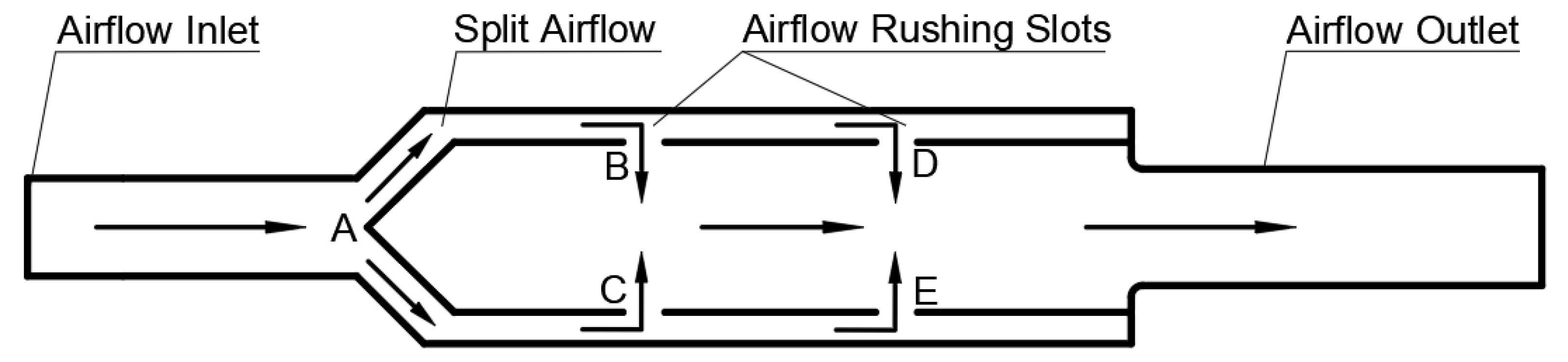
The working principle of the split-stream rushing muffler is illustrated in Figure 1 [5]. When airflow enters through the inlet, it is directed by the conical surface at point A into the ring cavity. From there, the airflow is divided into two groups and passes through the rushing slots at points B, C, and D, E. These two rushing airflows, moving at equal velocities but in opposite directions, converge and collide at the center of the inner cavity and effectively reduce the airflow velocity. Finally, the combined airflow exits through the tailpipe. This design achieves noise reduction and lowers exhaust resistance by decreasing the airflow velocity within the muffler.
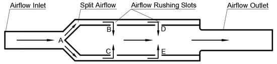
Figure 1.
The working principle of the split-stream rushing muffler.
This research focuses on a split-stream rushing exhaust muffler as its research object and employs COMSOL simulation software to perform relevant analyses of the structural modes, acoustic cavity modes, and coupled modes of the muffler. Furthermore, the impact of the acoustic–structural coupling effect on its acoustic performance was investigated using the acoustic finite element method, and the findings were validated experimentally. Based on this, a single-factor optimization study was performed on the structural parameters of this muffler. This investigation aimed to elucidate the patterns of influence of individual factors on transmission loss and to identify a muffler structural parameter configuration that yields better acoustic performance.
2. Basic Theories
2.1. Structural Modal Theory
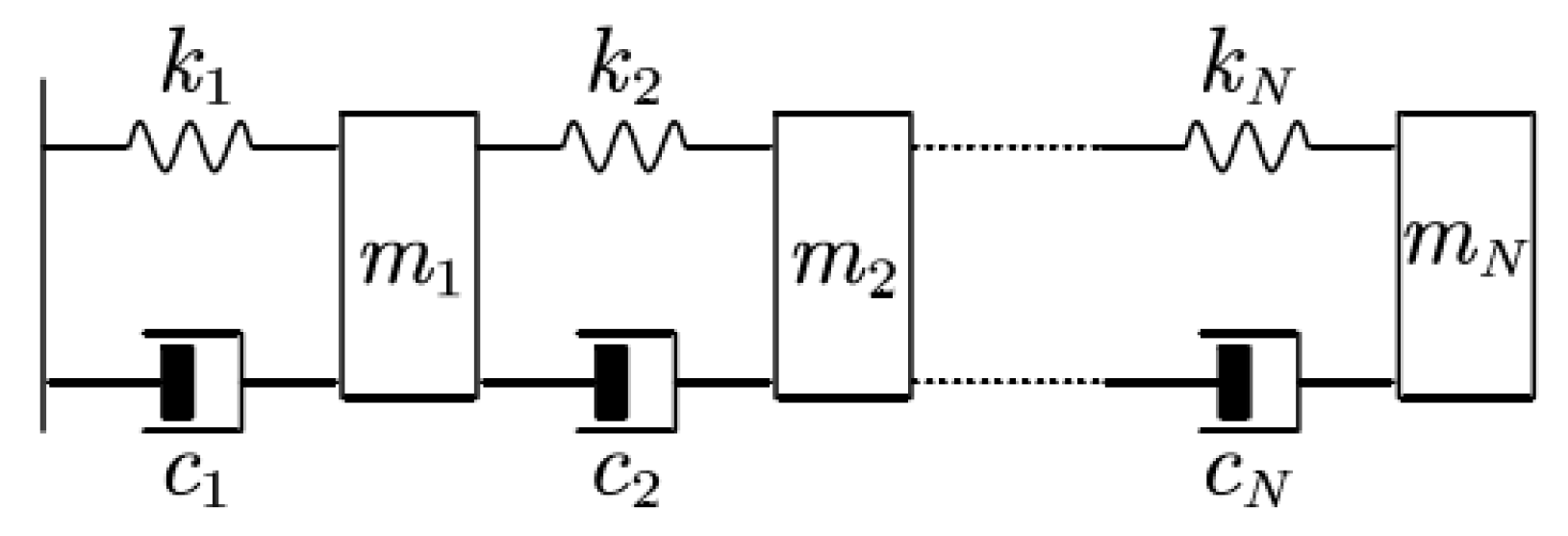
In this research, the diverted gas impingement muffler is treated as a multi-degree-of-freedom system, as illustrated in Figure 2.
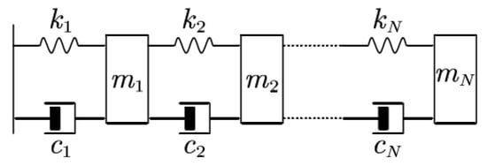
Figure 2.
Multiple-degree-of-freedom system.
The vibration equation for a linear, time-invariant system with multiple degrees of freedom can be represented as follows:
In the equation, represents the mass matrix of the multi-degree-of-freedom system, denotes the system damping matrix, denotes the system stiffness matrix, is the excitation vector at each point of the system, and , , and correspond to the acceleration vector, velocity vector, and displacement vector, respectively. Their definitions are provided below.
Given a small damping coefficient in the structural system, the muffler is treated as an undamped-free system, with the external structural system being free from external forces. Consequently, under free vibration, both its damping matrix and the excitation vector at each point of the system become zero, i.e., = 0, = 0, and the differential equation in Equation (1) simplifies to
Upon further analysis of Equation (4) and assuming the free vibration to be harmonic motion at this point, the subsequent equation is derived:
Substituting the aforementioned Equations (5) and (6) into (4) yields
2.2. Acoustic Cavity Modal Theory
The acoustic cavity mode represents a specific instance of the acoustic mode, typically focusing on the acoustic wave phenomena within enclosed or partially enclosed cavities, and the split-stream rushing exhaust muffler under discussion in this paper falls into this category. Consequently, the acoustic wave resonance within this muffler will be investigated via an acoustic cavity mode analysis.
The mode shape characteristics of acoustic cavity modes are characterized by the spatial distribution of sound pressure. Resonance amplification of the intracavity sound pressure will occur when the external excitation frequency approaches or coincides with the eigenfrequency of a specific acoustic cavity mode [17]. Particularly within the lower-order mode frequency spectrum, acoustic cavity modes and structural modes exhibit a higher susceptibility to coupling, consequently influencing both the acoustic performance and structural properties of the muffler.
Within acoustic cavity modes, the sound pressure in a uniform, source-free medium is governed by the following wave equation:
where denotes the speed of sound and is the Laplacian operator, signifying the second-order spatial derivative of a function, and its formula is given by
By incorporating the acoustic boundary conditions and discretizing Equation (4), the acoustic finite element equation for a non-viscous fluid medium is derived as follows:
In which denotes the acoustic mass matrix, denotes the acoustic stiffness matrix, denotes the acoustic damping matrix, denotes the sound pressure vector at the element nodes, and denotes the generalized load vector. If there is no sound wave attenuation in the sound field, then = 0. Furthermore, when computing the eigenvalues and eigenvectors for acoustic cavity modes, the generalized load vector should be zero. Consequently [18], Equation (10) simplifies to
The characteristic equation is then given by
where represents the acoustic cavity mode frequency. The linearly independent eigenvectors ( = 1, 2, 3…) and eigenvalues ( = 1, 2, 3…), which correspond to the mode shapes and modal frequencies of the acoustic cavity modes, can be obtained from the preceding equation.
2.3. Acoustic–Structural Coupling Modal Theory
Acoustic–structure coupling is a multi-physics analysis system that examines the interactions between solid structures and acoustic waves in air. This research method interprets the coupling process by solving the acoustic wave equation for the system under defined boundary conditions through classical acoustic analytical techniques.
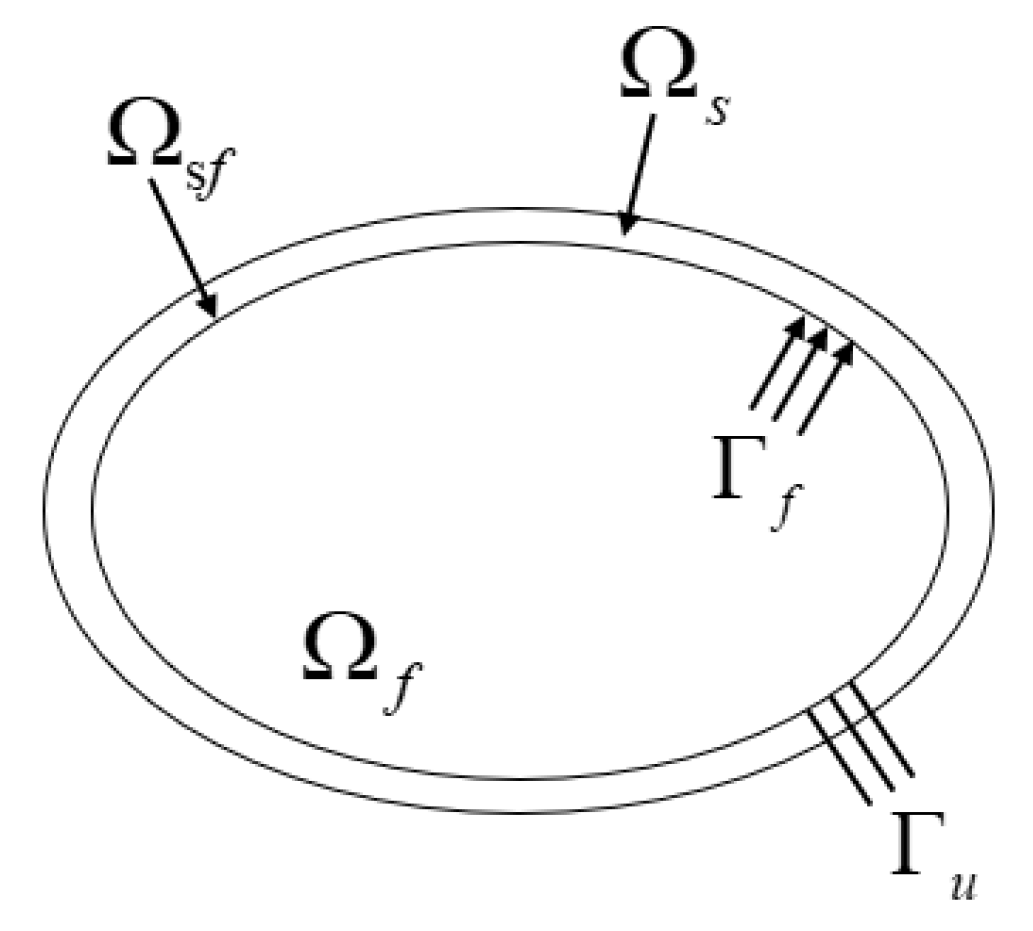
The diagram of the acoustic–structure coupling system is shown in Figure 3. The complete coupling system consists of a structural domain (), an acoustic cavity domain (), and a coupling interface (). The boundary conditions of domains include the pressure boundary condition () and displacement boundary condition () [19]. The structure and acoustic waves interact at the coupling surface between the solid structure and the acoustic cavity of the muffler. To ensure proper coupling, continuity of sound pressure and displacement must be maintained on the coupling surface. Therefore, the coupling process must satisfy the following conditions:
where is the displacement of the acoustic cavity domain at the coupling boundary, is the displacement of the structural domain at the coupling boundary, is the normal vector of the acoustic cavity surface at the coupling boundary, and is the normal vector of the structural surface, with the relationship = −.

Figure 3.
Diagram of the acoustic-structure coupling system.
At the coupling interface of the acoustic–structure system, the stress on the structural interface () and the sound pressure () are continuous. They are related by the following equation:
where is the normal projection of along the structural interface.
To verify the acoustic–structure coupling effect, establishing a coupling equation is necessary. The muffler consists of both structural vibration and an acoustic fluid domain. The differential equations governing the acoustic fluid domain and structural vibration, based on the fundamental acoustic equation, are as follows:
where and are the mass matrices of the fluid and structure, respectively. and are the damping matrices of the fluid and structure, respectively. and are the stiffness matrices of the fluid and structure, respectively. is the sound pressure vector at the unit nodes, is the displacement at the structural unit node, is the fluid load, and is the external incentive of the system.
Considering the coupling effect between the structure and acoustic fluid, the differential equation of the system must incorporate the influence of coupling forces, including the force exerted by sound pressure on the structure and the force due to structural movement on the acoustic cavity. To account for these forces in the equation, they must be treated as applied external loads. The differential equations for the structural domain and acoustic cavity domain of the coupling system are as follows:
According to the continuity condition, if the nodes of the acoustic cavity domain correspond one-to-one with the nodes of the structural domain on the coupling boundary, the force exerted by the acoustic domain on the coupling interface () and the force exerted by the structural domain on the coupling interface () can be expressed as follows:
where is the Lagrange shape function of the isoparametric hexahedral element in the acoustic cavity domain, is the Lagrange shape function of the isoparametric tetrahedral element in the structural domain, and represents the coupling boundary.
is the acoustic–structure coupling matrix and it can be expressed as follows after introducing the system–space coupling matrix [20]:
Equation (21) is substituted into Equations (19) and (20). Consequently, Equations (19) and (20) can be simplified as follows:
The finite element equation of the acoustic–structure coupling system can be obtained by combining Equations (17)–(23):
Assuming that both displacement and acoustic waves are harmonic functions, Equation (24) can be rewritten as a formula without the differential term [21]:
In Equation (25), the sound pressure and displacement of the acoustic–structure coupling system are solved using the direct coupling method. However, the left coefficient matrix is asymmetric, which results in heavy computational load and long solving times. To address these issues, the mode superposition method is introduced. Superimposition of the structural and acoustic modes of the system leads to the following expression:
where is the uncoupled structural vibration matrix of the system, also known as the structural modal matrix; is the uncoupled acoustic matrix of the system, also known as the acoustic modal matrix; and and are the participation factors of the structural and acoustic modes, respectively.
Equations (26) and (27) are substituted into Equations (24) and (25), resulting in the following:
The parameters in the above equations are
2.4. Acoustic Attenuation Performance
Acoustic attenuation performance is typically evaluated by transmission loss, which refers to the difference between the incident sound power level at the inlet and the transmitted sound power level at the outlet of the muffler (measured in dB). The formula for calculating transmission loss is
From Equation (31), assuming total silence at the airflow outlet of the muffler, the transmission loss is the difference between the incident sound power level and the transmitted sound power level of the muffler [22]. The amplitude of the function reaches its maximum at the midpoint of the source field and is zero at both ends. The subscripts ‘1′ and ‘2′ represent the forward and backward traveling waves, respectively. refers to the incident sound power level of the muffler, while refers to the transmitted sound power level. represents the incident sound power, and represents the transmitted sound power. refers to the incident sound pressure, and refers to the transmitted sound pressure (Figure 3). is expressed as the sum of and .
Suppose that only a plane wave exists at both the upstream and downstream ends of the muffler, then the relationship between sound pressure and particle velocity () can be expressed as follows:
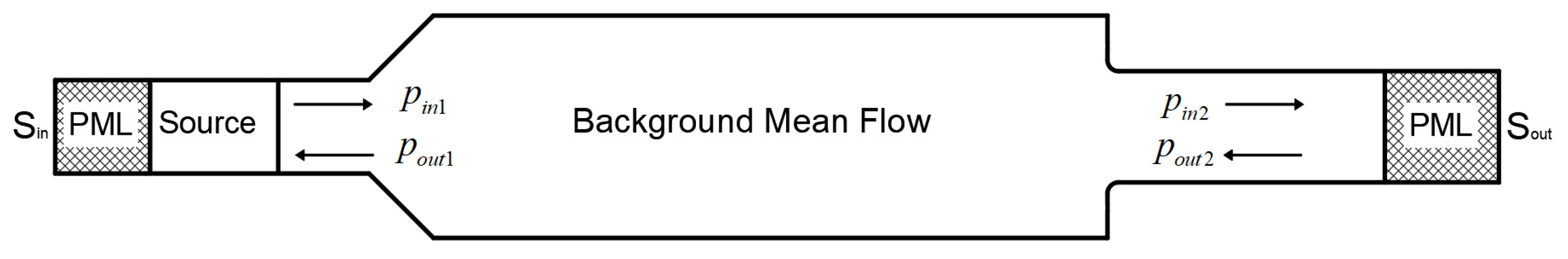
In Figure 4, and represent the cross-sectional areas of the muffler’s inlet and outlet, respectively. For an accurate evaluation of the muffler’s acoustic attenuation performance, perfect matching layers are applied at both the upstream and downstream ends. These layers absorb the reflected and transmitted acoustic waves, respectively, reduce boundary effects, and enhance the calculation stability.

Figure 4.
Diagram of the incident sound power level and transmitted sound power level.
3. Numerical Calculation
3.1. Physics Interface
Within the COMSOL software, the theoretical model developed in Section 2 is realized through the “Acoustic–Shell Interaction” physics interface. The “Acoustic–Shell Interaction” interface couples the “Pressure Acoustics, Frequency Domain” and “Structural Mechanics, Shell” physics modules. The bidirectional coupling between them at their shared boundary is achieved through COMSOL’s “Acoustic–Structure Boundary” interface, which ensures the accurate expression of the interaction between the sound field and the structural field. In the course of conducting the finite element simulation for this module, the system will automatically generate Formula (29) derived from the theoretical model. Furthermore, this numerically maps the stiffness matrix, mass matrix, damping matrix, and the associated coupling terms of the coupled system, thus enabling the discretized solution of the control equations governing acoustic–structure coupling.
3.2. Simulation Model Building of the Split-Stream Rushing Muffler
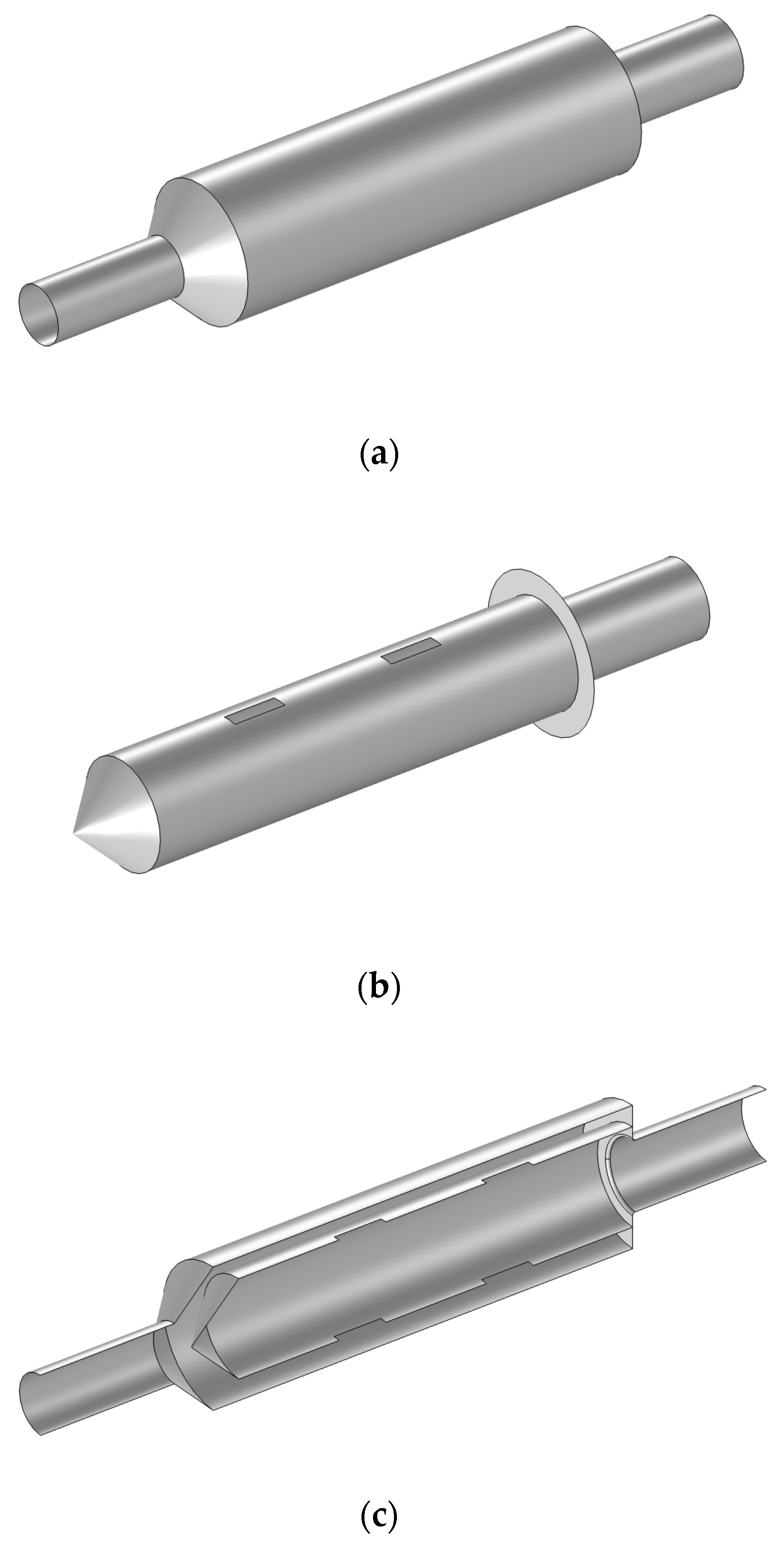
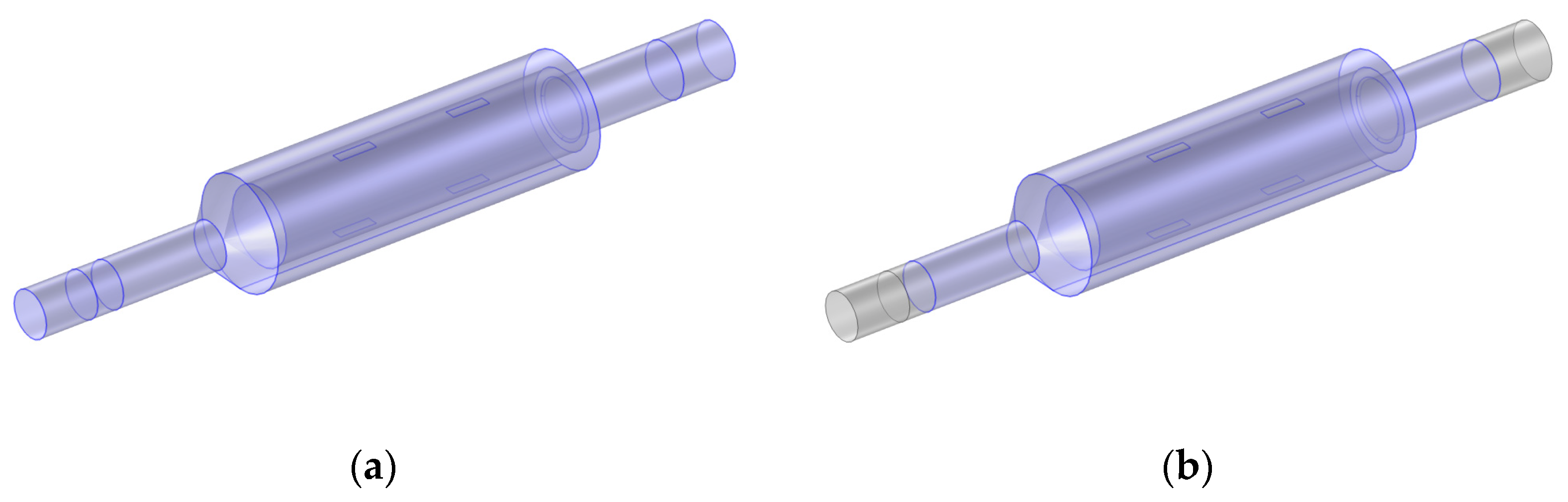
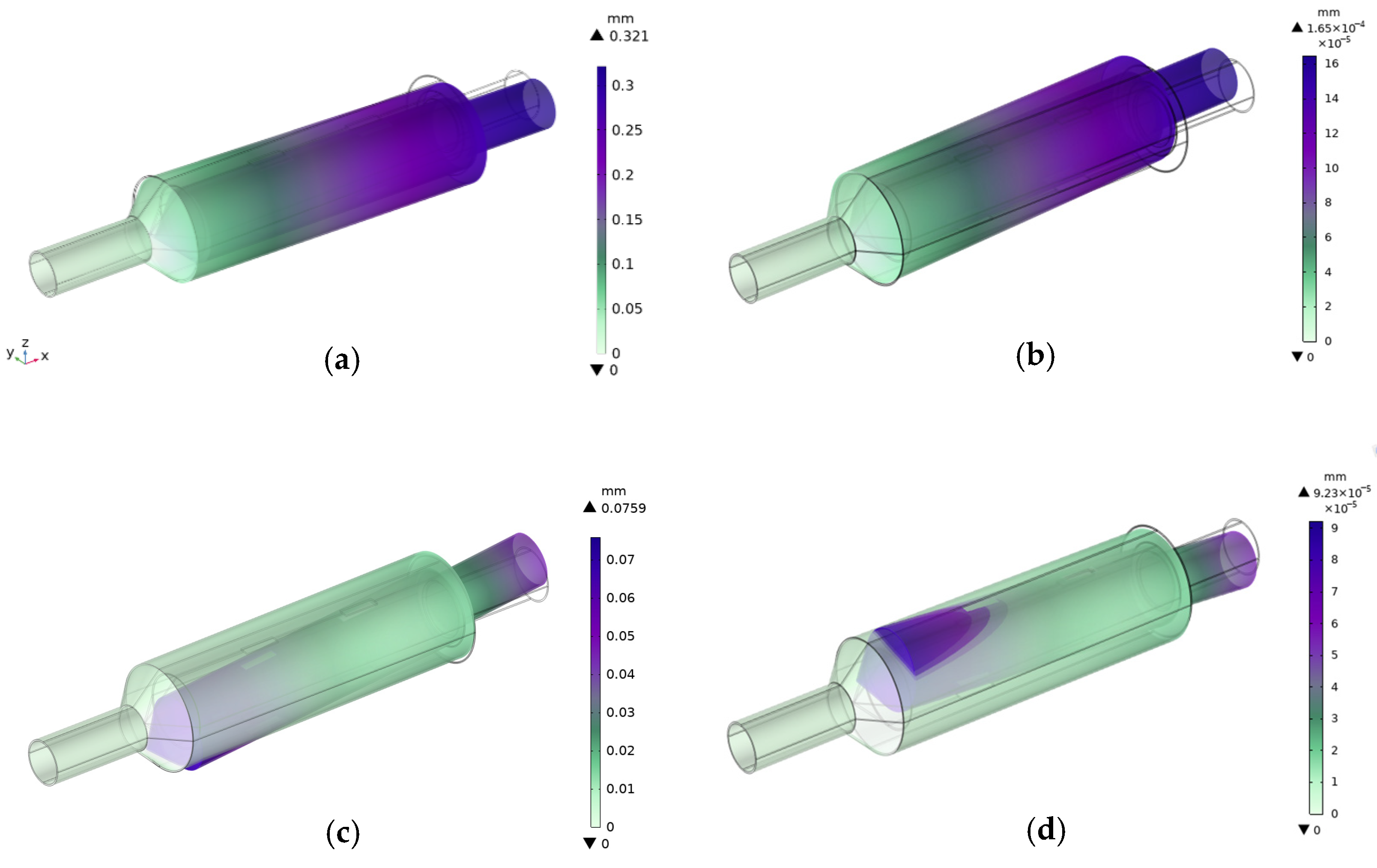
The split-stream rushing muffler as a whole comprises inner and outer sections. The inner and outer tubes are connected at their ends via steel bar supports. For finite element modeling purposes, these two sections are treated as a single entity. The model is depicted in Figure 5.

Figure 5.
Three-dimensional model of the muffler with acoustic–structure coupling. (a) Overall structure, (b) Inner tube, (c) Cross-section.
When the model contains a heterogeneous structure, it can be handled by applying refined meshing, reasonable simplifications, and accurate definitions of the materials’ properties. The tapered surface of the muffler’s inner tube is a heterogeneous structure element. In the model, this angle is 90°. However, during actual manufacturing, due to production reasons, the sharp angle has become rounded due to welding marks. This rounded section needs to be replicated in the model (Figure 6).
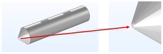
Figure 6.
Rounded conical angle of the rushing unit.
After processing the heterogeneous structure, verifying the changes is necessary to ensure they do not affect the accuracy of the simulation results. Therefore, the mass, aspect ratio, and Jacobian ratio of the grid cells are selected as evaluation indicators for unit discretization before and after processing the structural heterogeneity. The comparison between the rectangular and rounded conical angles is shown in Table 1.

Table 1.
Comparison of unit discretization for rectangular and rounded conical angles.
In Table 1, the unit mass error between the rounded conical angle and the rectangular conical angle is within ±1.14%, indicating that the structural change has a minimal impact on the simulation accuracy.
3.3. Material Definition
Using the established model, the computational region was partitioned into the air domain and the structural domain. As shown in Figure 7, the air domain encompasses two PMLs located at the front and rear, along with the intermediate background pressure field region, and the structural domain encompasses solely the wall portion of the muffler. In terms of the material property configuration, the material for the air domain is defined as air, while the structural domain utilizes 06Cr19Ni10 steel.
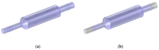
Figure 7.
Regional map of muffler material properties. (a) Acoustic domain, (b) Structural domain.
The 06Cr19Ni10 material chosen is capable of satisfying the diverse experimental demands in the muffler design and development process; the material’s attributes are presented in Table 2.
Table 2.
Material properties of 06Cr19Ni10.
3.4. Meshing
For finite element analysis, the characteristic length of acoustic mesh elements must be no greater than one-sixth (1/6) of the smallest acoustic wavelength to guarantee the precision of the acoustic simulation. The formula is given below.
Given that the exhaust noise frequency is below 5000 Hz, the maximum characteristic length of the acoustic mesh elements, as determined by the formula, should be less than 19 mm. Consequently, the maximum acoustic mesh element size for the muffler was defined as 8 mm, and the minimum size was 5 mm. The acoustic domain exhibits low sensitivity to boundary data, and thus it was configured with two layers, featuring a first layer wall boundary layer thickness of 0.3 mm. Concurrently, the mesh around the four rushing holes on the muffler’s inner tube was locally refined, with a maximum acoustic mesh element size of 3 mm. To enhance the acoustic mesh quality, a swept meshing technique was applied to the regular cylindrical volumes at the inlet and outlet of the muffler, resulting in hexahedral elements. After the above operations, the resulting mesh comprised a total of 209,157 elements, as shown in Figure 8.
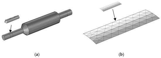
Figure 8.
Three-dimensional acoustic mesh of the muffler geometry. (a) Acoustic mesh of the muffler, (b) Acoustic mesh of the muffler’s inner tube.
3.5. Boundary Condition
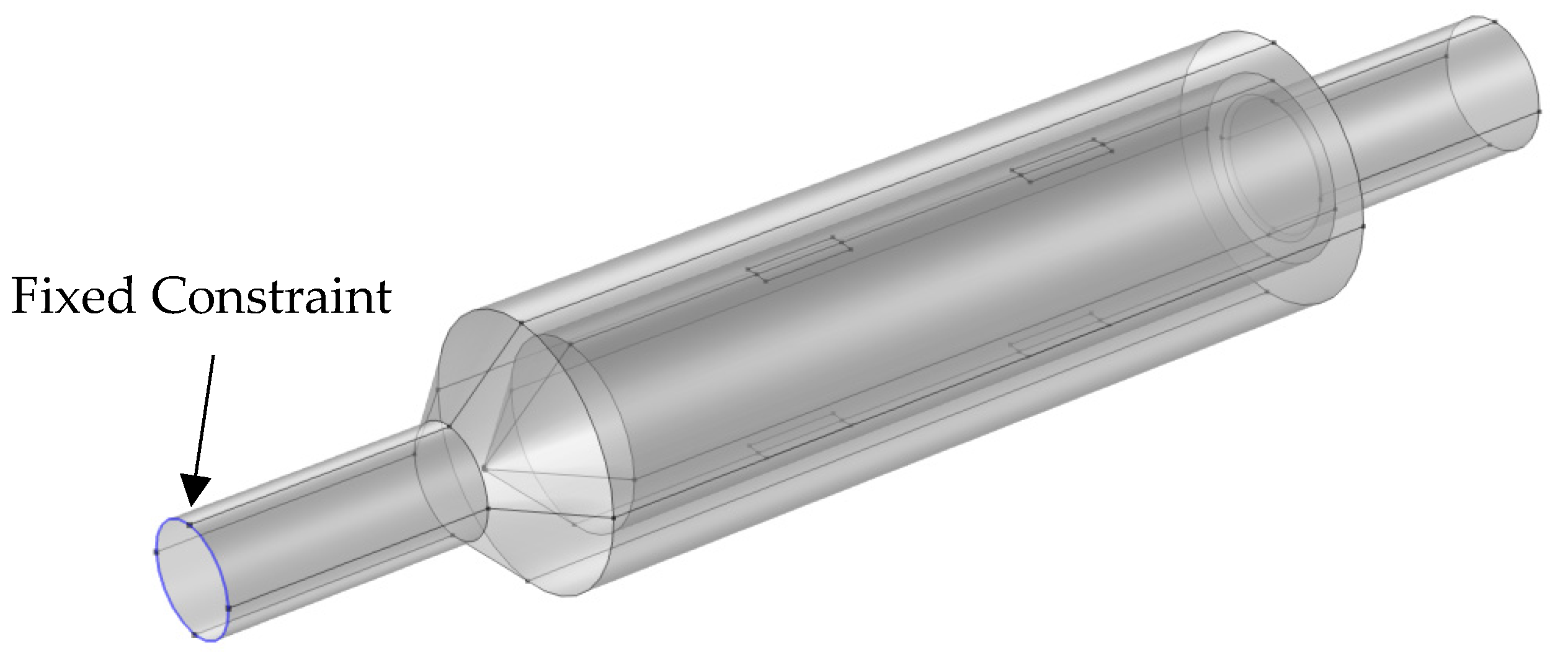
3.5.1. Structural Boundary Condition
As shown in Figure 9, a fixed constraint typically signifies that the displacement at the boundary is completely restricted, whereby all degrees of freedom on the boundary are set to zero. This signifies that the material points on the boundary will not experience any displacement. Within structural mechanics, the mathematical representation of a fixed constraint is as follows:
Figure 9.
Schematic diagram of fixed constraints.
In the case of an exhaust muffler, as its inlet requires connection to the engine exhaust port, the displacement at the inlet is therefore negligible.
3.5.2. Acoustic Boundary Condition
- (1)
- Sound hard boundary (wall)
Before conducting the finite element analysis of the muffler, the establishment of boundary conditions is required to solve the acoustic differential equations and integral equations.
where represents the fluid density, denotes the total pressure, and signifies the zero dipole domain source. Given a zero dipole domain source = 0 and a constant fluid density , this implies that the normal derivative of the pressure at the boundary must be zero, resulting in
- (2)
- Interior sound hard boundary (wall)
As the split-stream rushing muffler is comprised of an inner tube and an outer tube, during the establishment of boundary conditions, designating the inner tube as a sound hard boundary is necessary.
Equations (39) and (40) are, respectively, applicable to the upper and lower surfaces of the boundary, as demonstrated by the subscripts of the equations. Analogous to the sound hard boundary condition, given a zero dipole source and a constant fluid density , the normal derivative of the pressure is likewise zero at the boundary.
4. Experimental Verification
4.1. Test Method
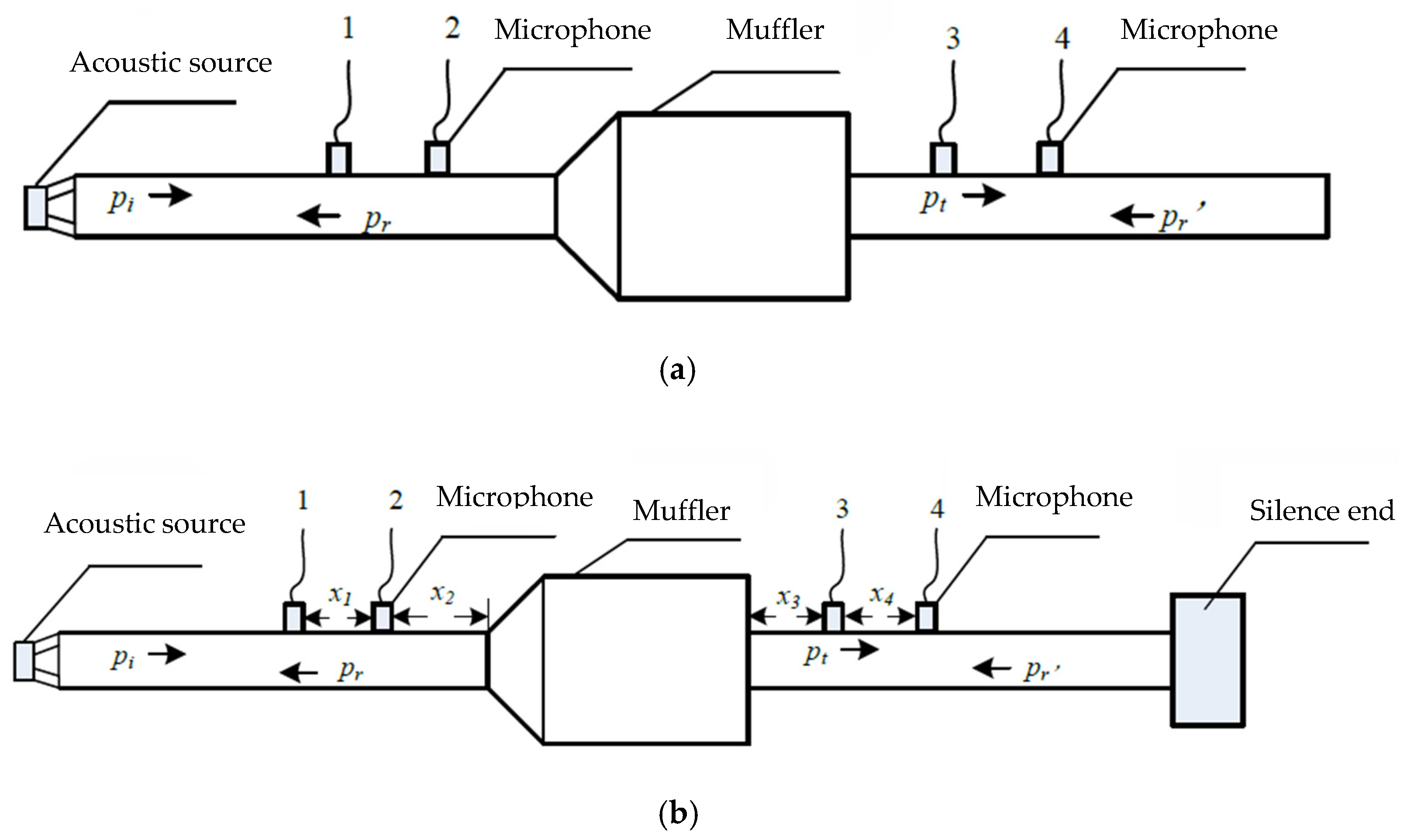
The two-load method is easy to operate because it requires only a change in resistance at the outlet of the muffler without the need to adjust the sound source position at the inlet. Hence, this method is used in the experiment for this section. The experiment incorporated two distinct impedance boundary conditions at the muffler’s exhaust outlet: an open-end condition and a condition with a fully anechoic termination. Corresponding equation sets were established through the two conditions. Subsequently, the outcomes from these systems were introduced, enabling the determination of the four-pole parameters and the subsequent derivation of the transmission loss [23]. The test principle of the two-load method is illustrated in Figure 10.
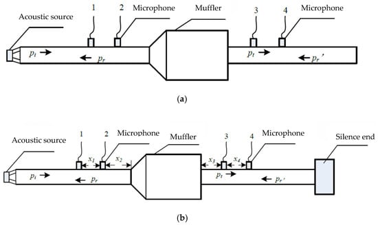
Figure 10.
Diagram of the two-load method. (a) Without a silenced end, (b) With a silenced end.
In the two-load test method shown in Figure 10, the relationship between the acoustic waves at both ends of the muffler is expressed as follows:
where and on the left represent the upstream incident wave and reflected wave, respectively. and represent the downstream transmitted wave and reflected wave, respectively. , , , and are the quadrupole parameters of the transmission matrix.
According to the definition of transmission loss and the test principle of the two-load method, the outlet of the muffler must be a non-reflective end, meaning that = 0. Therefore, the transmission loss using the two-load method can be expressed as follows:
As seen from Equation (42), under general test conditions, it is difficult to achieve a non-reflective end downstream of the muffler. Therefore, establishing two sets of equations by varying the loads at the outlet of the muffler is necessary to solve for in Equation (42).
For Figure 10a, where the outlet is open, the equation set is
For Figure 10b, where the outlet is a total silenced end, the equation set is as follows:
A combination of Equations (43) and (44) results in the following equation:
where subscripts and of represent the two different terminal loads of the muffler. During the two-load test, two microphones are placed in front of and at the back of the muffler to separate the incident and reflected waves. The sound pressure signals measured by the four microphones can be used to distinguish between the sound pressures of the advancing wave and the reflected wave by changing the loads at the muffler outlet. These measurements are then substituted into Equation (45) to calculate . Finally, the transmission loss of the muffler can be determined using [24,25].
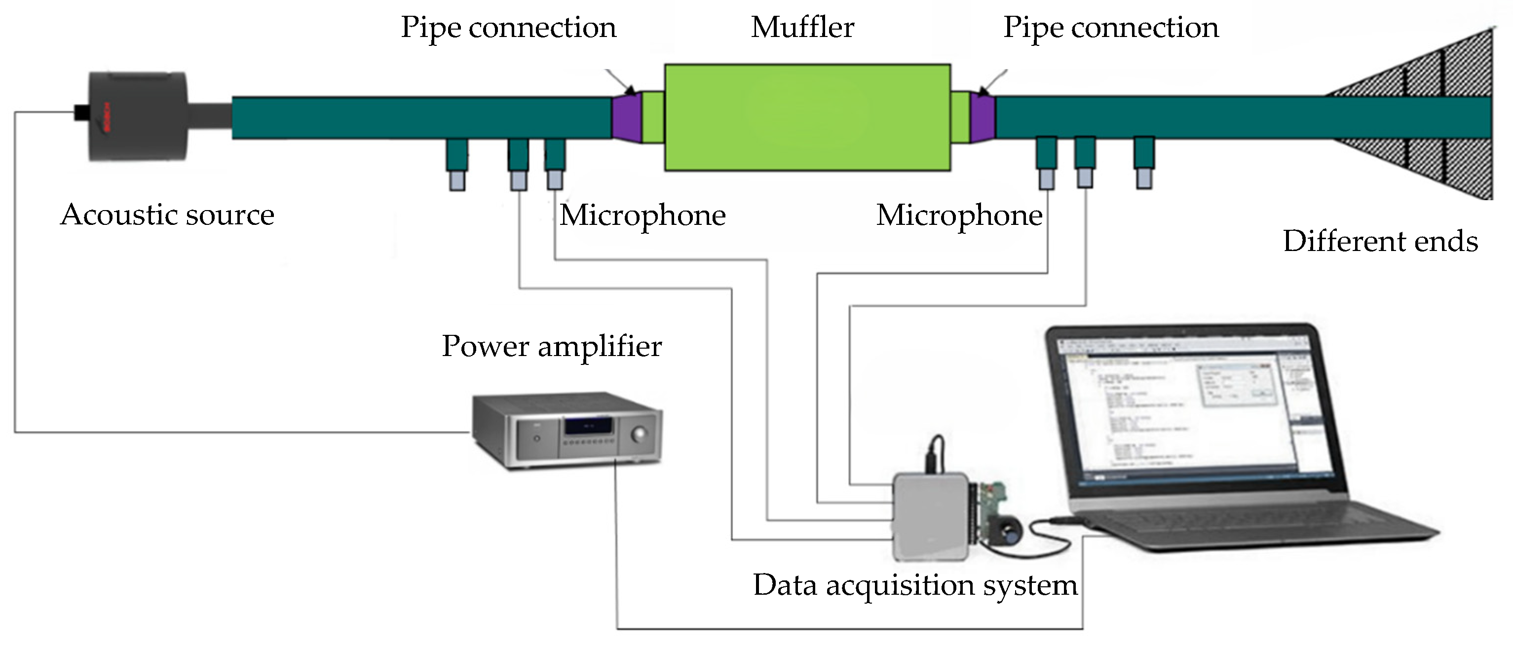
4.2. Construction of the Testbed
The airflow-free acoustic performance test system for the muffler is shown in Figure 11. This testbed is mainly composed of the noise generator and testing system, which includes the sound source, microphones, acoustic acquisition system, muffler test specimens, and terminal muffler. It is designed to evaluate the acoustic attenuation performance of the split-stream rushing muffler. Specifically, the microphone used was an MPA201 (1/2 inch, BSWA Technology Co., Ltd., Beijing, China) sensor, the impedance tube was a CIT30 model, and the acoustic data acquisition system employed a BOACH-DRH-DR08 data acquisition card.

Figure 11.
Assembly of the transmission loss testbed and devices.
In this test system, the sound source is provided by a loudspeaker. The sound source signals are generated by the signal generation module of the multi-channel data acquisition and analysis device and are amplified by the power amplifier. At the outlet section, different resistive loads are applied for several measurements, as the transmission loss of the split-stream rushing muffler is tested using the two-load method. The first loading condition involves no additional loads, while the second loading condition includes additional loads of cross-sectional pipes with sudden resistance expansion to achieve varying test loads.
The positions of the four microphones on the pipe are determined according to the standards ASTM E1050-98 and GB/Z 27764-2011 [26,27]. Meanwhile, the sensing films of the microphones are kept aligned with the pipe wall of the testbed. The distance between each pair of microphones and the highest frequency in the test must satisfy the following condition:
where is the sound velocity, is the highest test frequency, and is the distance between two microphones. In general, should be small for testing high-frequency signals but large for testing low-frequency signals. According to earlier studies on the split-stream rushing muffler, this research focuses on low-frequency signals. Therefore, is set to 30 mm and is approximately 5667 Hz. Microphones are installed at the same positions on both the upstream and downstream sections, with the shortest distance between the two pairs of microphones and the muffler being 130 mm.
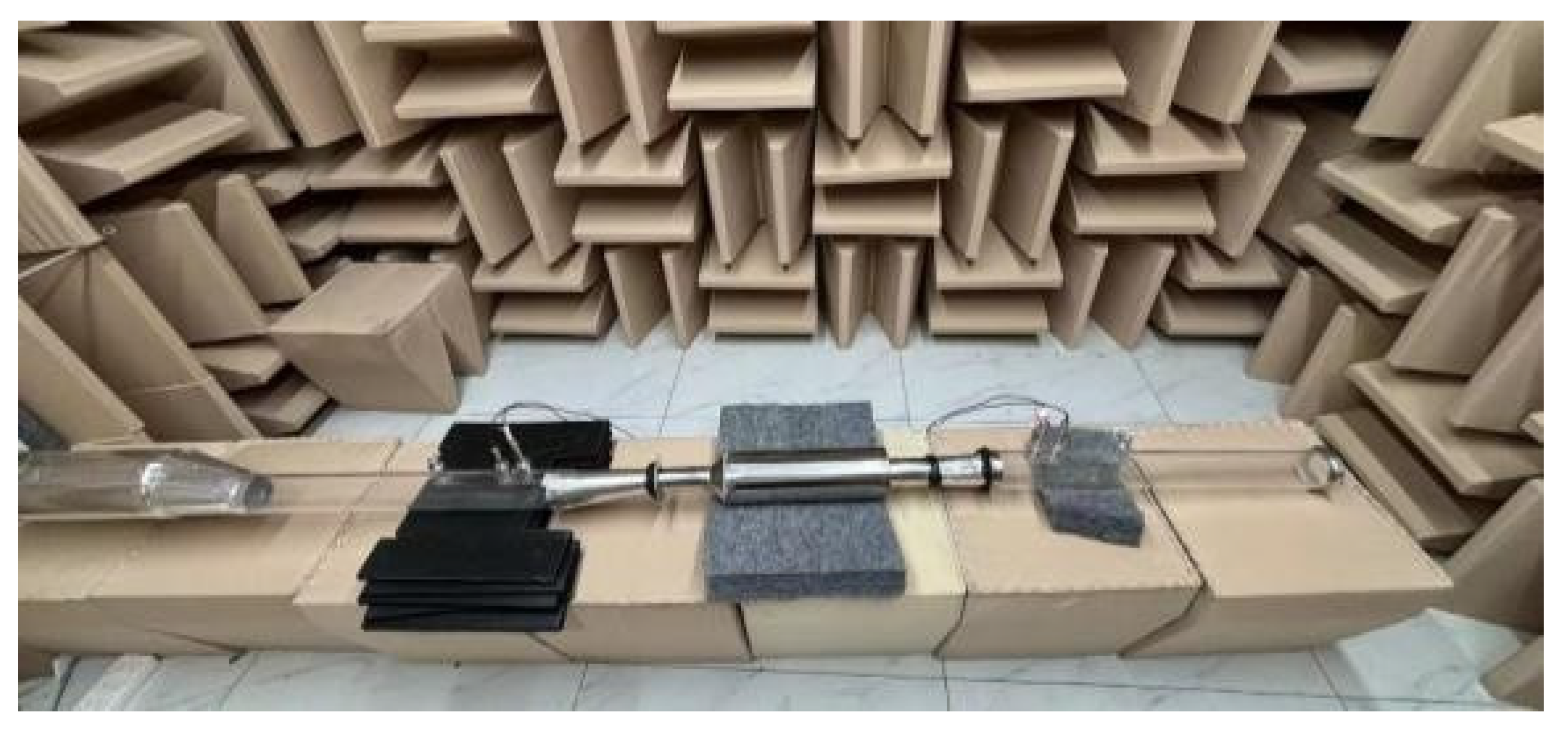
As depicted in Figure 12, the sound source is placed outside of the anechoic chamber during the construction of the testbed, while the remaining components are positioned inside to reduce disturbances to the acoustic test. Before testing, verifying whether the background noise in the pipes met the test conditions was necessary. During the airflow-free transmission loss test, the loudspeaker is first turned off, and the background noise level in the pipes is about 48 dB. Subsequently, the loudspeaker is turned on, and the measured sound pressure level of the noise at the same pipe position is about 70 dB. The sound pressure level difference between the sound source signals and the background noise exceeds 10 dB, which satisfies the test requirements of GB/T 4759-2009 [28]. During the measurement, the temperature in the pipes is 30 °C, while = 343 m/s and .
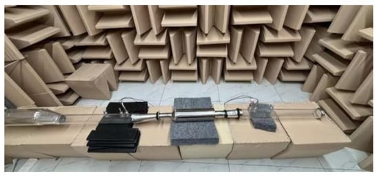
Figure 12.
Field test setup of the testbed.
During the transmission loss test, calibrating the microphones is essential to ensure the accuracy and repeatability of the test results. First, it must be confirmed that the microphones and calibration equipment (e.g., acoustic calibrators or standard microphones) are in proper working condition and within their calibration period. Following this, the microphones are calibrated according to the steps outlined below. (1) Connect the microphones to the test system (e.g., frequency analyzer or sound level meter). (2) Insert the microphones into the acoustic calibrator and ensure a proper seal to prevent sound leakage. (3) Turn on the acoustic calibrator and apply signals with known sound pressure levels (e.g., 90 dB SPL). (4) Read and record the outputs of the microphones in the test system. (5) If applicable, adjust the system’s sensitivity to ensure consistency between the displayed sound pressure level and the calibrator’s sound pressure level. (6) Repeat the above steps at least three times to ensure the consistency of the numerical values. The accuracy of the microphones can be ensured by following these calibration steps [29]. To reduce test errors, the connectors of the split-stream rushing muffler and the resistance pipe must also be sealed during the test.
5. Acoustic–Structural Coupling Analysis of the Muffler
5.1. Structural Modal Analysis
Within the structural modal analysis procedure, as the objective is to determine the free vibration modes of the structure, and considering the actual mounting configuration of the muffler, prestress is not required. Only the muffler’s inlet needs to be constrained, while its outlet remains unconstrained and requires no further boundary conditions. The first eight structural modes are shown in Table 3. Typically, lower frequency vibrations exert the most significant influence on both the acoustic behavior and the structural response characteristics of mufflers. This is attributed to the fact that lower frequency modes, associated with lower frequency vibrations, possess greater energy and have a more substantial contribution to the structural dynamic response and acoustic radiation. Moreover, the majority of noise and vibration concerns are prevalent in the lower frequency spectrum, and lower-order modes are more representative of the crucial dynamic behaviors of mufflers [30].
Table 3.
Structural mode parameters of the split-stream rushing muffler.
Degenerate modes arise due to the structural geometric symmetry, exhibiting closely spaced modal frequencies and highly similar mode shapes. Consequently, as shown in Table 3 and Figure 13, the initial eight modes exhibit the presence of three sets of degenerate modes, specifically the first and second modes, the third and fourth modes, and the seventh and eighth modes. The modal vibration patterns of the first to sixth orders exhibit transverse motion, characterized by translational, swinging, and torsional movements of the muffler’s partial shell, displaying relatively simple mode shapes. The first and second modal orders are characterized by the translational motion of the muffler’s outer casing in the y-direction. The third and fourth modal orders are characterized by the swinging motion of the muffler’s inner tube within the x-y plane. The fifth modal order is characterized by the torsional motion of the muffler about the positive y-axis. The sixth modal order is characterized by the translational motion of the muffler’s inner tube in the positive x-direction. From the seventh modal order onwards, the modal vibration patterns exhibit increased complexity. The seventh and eighth modal orders are characterized by the elongation and contraction of the muffler’s outer casing within the y-z plane. In general, the modal vibration patterns exhibit increasing complexity with ascending modal order. This is primarily attributed to the fact that the elevation of the system frequency results in a greater number of degrees of freedom, coupled with a more pronounced influence of both the mass and stiffness matrices. Moreover, the model’s eigenfrequencies and mode shapes are directly influenced by the mass distribution and stiffness distribution. Consequently, the system’s eigenfrequencies and their associated eigenvectors also undergo corresponding alterations.

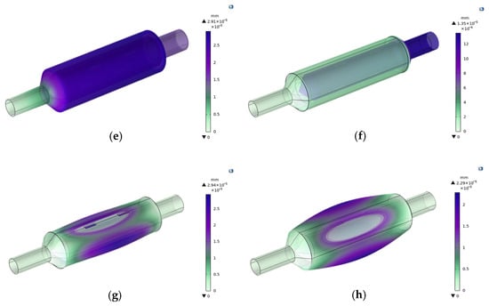
Figure 13.
The first 8 structural mode shapes of the split-stream rushing muffler. (a) 1st order, (b) 2nd order, (c) 3rd order, (d) 4th order, (e) 5th order, (f) 6th order, (g) 7th order, (h) 8th order.
5.2. Acoustic Cavity Modal Analysis
The results of the acoustic cavity modal analysis of the muffler are presented in Table 4 and Figure 14.
Table 4.
Acoustic cavity mode parameters of the split-stream rushing muffler.
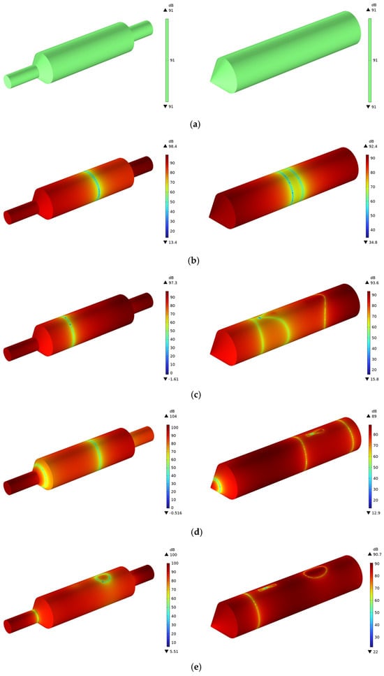
Figure 14.
The first 8 acoustic cavity mode shapes of the split-stream rushing muffler. (a) 1st order, (b) 2nd order, (c) 3rd order, (d) 4th order, (e) 5th order, (f) 6th order, (g) 7th order, (h) 8th order.
Figure 14 illustrates the sound pressure level cloud maps for the first eight acoustic cavity modes of the split-flow impingement muffler. For improved visualization of the sound pressure level distribution within both the internal and external cavities of the muffler, the sound pressure level cloud map of the muffler’s inner cavity was selected separately in the result processing.
As shown in Figure 14a, the first acoustic cavity mode exhibits a modal pattern characterized by uniform sound pressure throughout the entire acoustic domain. This typology bears resemblance to rigid body modes in structural dynamics, possessing only one degree of freedom, namely, sound pressure, throughout the entire muffler volume. This specific mode is exclusive to the first acoustic cavity mode and, therefore, holds no significance for the present investigation. Transverse acoustic modes begin to manifest from the second mode, and a transition from transverse to longitudinal acoustic modes occurs starting with the seventh mode. With the continuous increase in frequency, the sound pressure distribution within the muffler progressively becomes more intricate. Despite the increasing dispersion of the sound pressure level distribution across the first eight modes with ascending mode number, a general tendency for lower sound pressure levels within the muffler’s inner cavity compared to its outer cavity is observed. The occurrence of this phenomenon is primarily attributed to the unique structural design of the split-stream rushing muffler, wherein the internal configuration presents a geometric structure analogous to an expansion chamber. This configuration induces the scattering and reflection of acoustic waves, leading to the creation of regions with diminished sound pressure levels.
5.3. Acoustic–Structure Coupling Modal Analysis
Relevant computations for the sound–structure coupled modes of the split-stream rushing muffler were conducted using the “Acoustic–Shell Interaction, Frequency Domain” module within COMSOL. The first 10 coupled modes are presented in Table 5. As shown in Table 5, the frequencies of the second through fifth and the seventh coupled modes are essentially in agreement with the frequencies of the first to fifth structural modes, suggesting that the primary contribution to these coupled modes originates from the structural modes. Conversely, the frequencies of the sixth and eighth coupled modes are essentially in agreement with the frequencies of the second and third acoustic cavity modes, suggesting that this part of coupled modes is primarily governed by the acoustic cavity modes. This indicates that the frequency spectrum of the coupled modes is predominantly governed by the synergistic interaction of structural and acoustic cavity modes, and the coupled system, to some extent, preserves the modal attributes of its constituent subsystems. However, the ninth and tenth coupled modes did not exhibit a frequency correspondence with any individual structural or acoustic cavity mode, demonstrating prominent modal shift characteristics. This phenomenon arises from the enhanced interaction between the structure and the acoustic field within this frequency range, resulting in modal coupling and the emergence of novel modal shapes and frequency distributions that no longer entirely represent the properties of the individual subsystems. This indicates that within a particular frequency range, the coupling effect between the structure and the acoustic field becomes more pronounced, resulting in alterations of varying magnitudes in the inherent modal configurations and frequencies.
Table 5.
The first 10 acoustic–structural coupled modes of the split-stream rushing muffler.
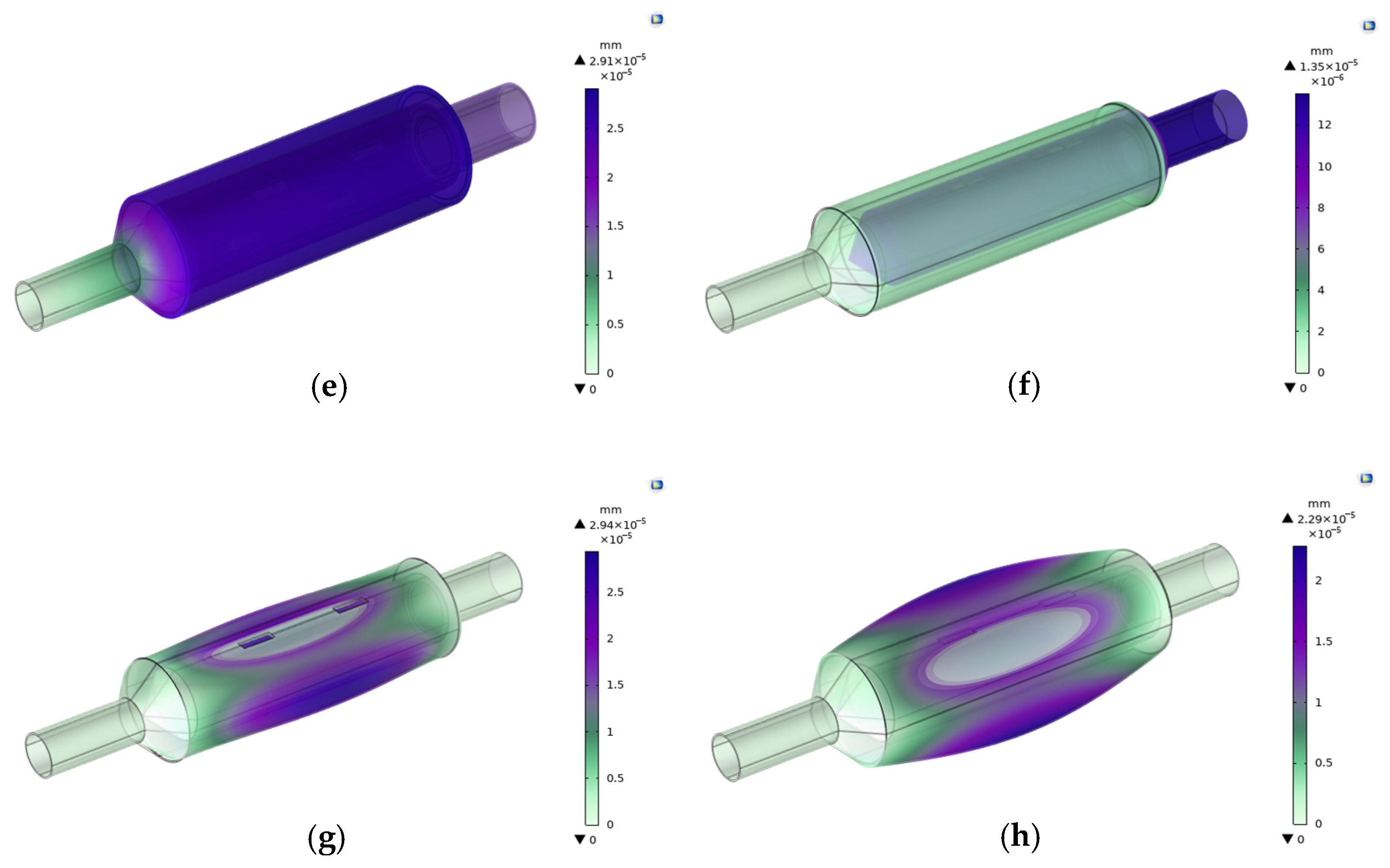
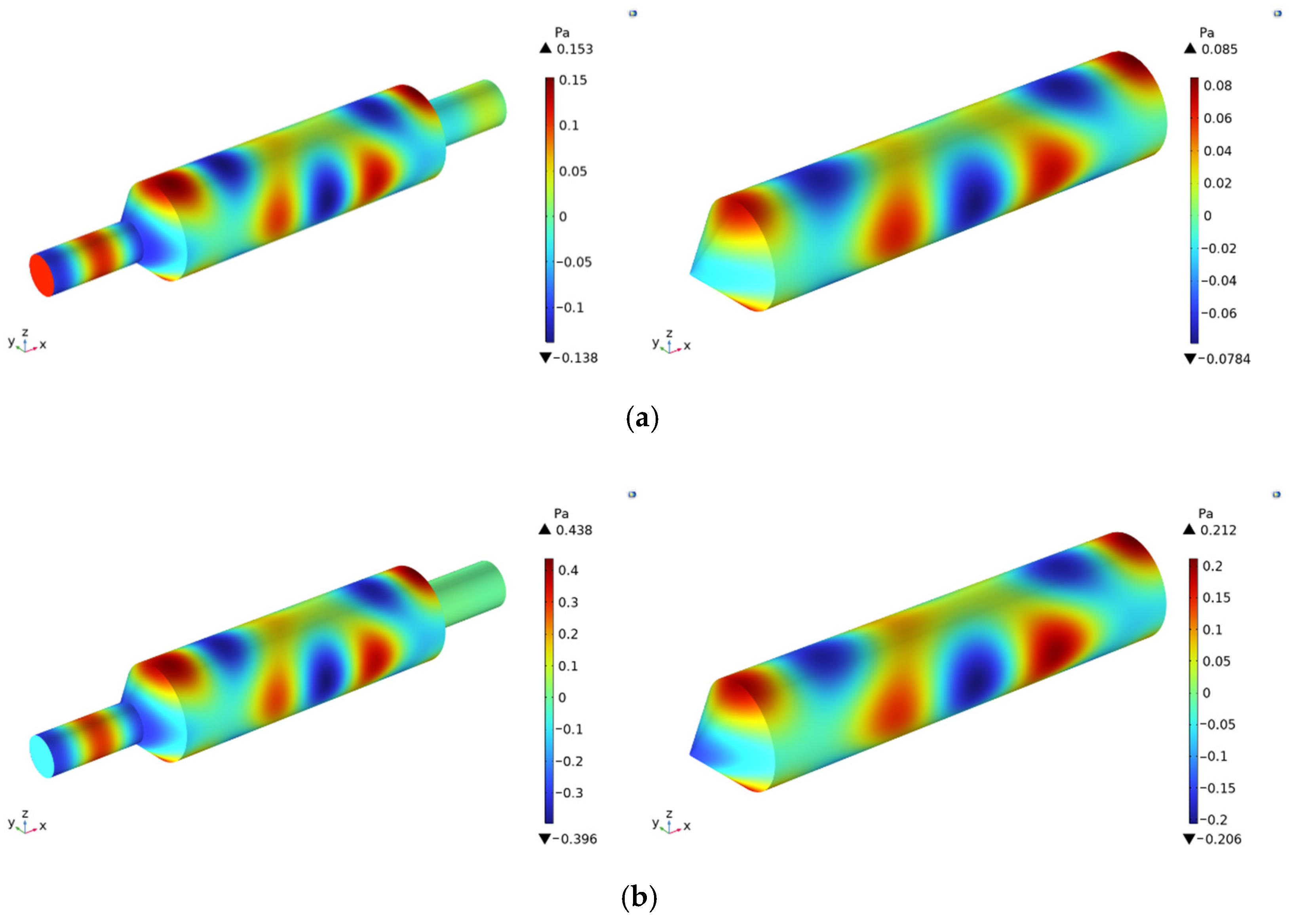
Figure 15 and Figure 16 illustrate comparative diagrams of coupled modes versus structural modes and acoustic cavity modes at proximate frequencies. The observation of both figures reveals that structural modes and coupled modes exhibit identical mode shapes at proximate frequencies. The distinction lies in the fact that the coupled mode shapes display partial torsional deformation in their phase relationship relative to the structural mode shapes. Acoustic cavity modes and coupled modes exhibit a high degree of resemblance in their modal configurations, sound pressure distribution locations, and sound pressure amplitudes at proximate frequencies.

Figure 15.
Comparison of some structural modes with coupled modes. (a) 2nd order coupled mode (82.38 Hz), (b) 1st order structural mode (82.43 Hz), (c) 7th order coupled mode (139.97 Hz), (d) 4th order structural mode (140.23 Hz).
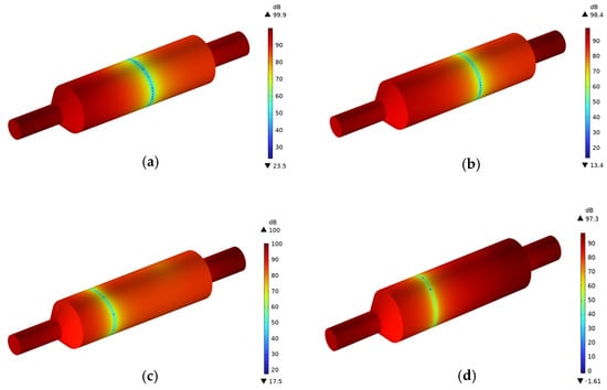
Figure 16.
Comparison of some acoustic cavity modes with coupled modes. (a) 6th order coupled mode (426.62 Hz), (b) 2nd order acoustic cavity mode (427.04 Hz), (c) 8th order coupled mode (570.78 Hz), (d) 3rd order acoustic cavity mode (571.1 Hz).
5.4. Analysis of Acoustic Attenuation Performance
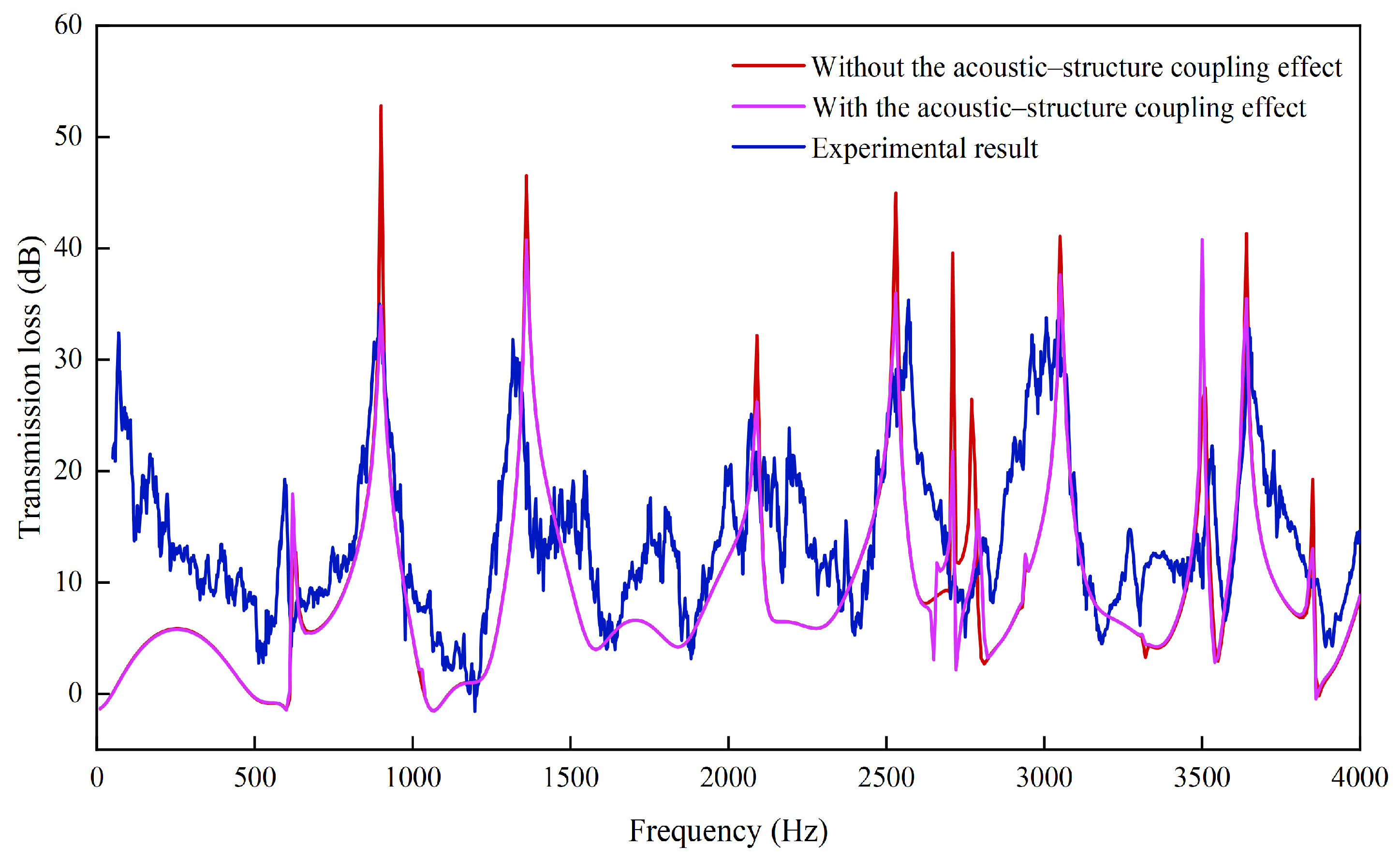
Figure 17 illustrates a comparative diagram of transmission loss. As shown in Figure 17, the experimental results exhibit closer agreement with the transmission loss considering sound–structure coupling effects than with the transmission loss neglecting these effects. Furthermore, the overall trends demonstrate better consistency, suggesting that the inclusion of sound–structure coupling effects enhances the accuracy of the finite element prediction of transmission loss. The above results can be analyzed as follows: The acoustic–structure coupling effect accurately reflected the interaction of acoustic waves during transmission between solid and air and captured resonance phenomena in the structure, as well as the frequency-dependent energy transmission patterns. These capabilities enabled a more precise description of the transmission loss characteristics. Moreover, the coupling model better simulated the complex boundary conditions in the test and showed particularly high prediction accuracy in both low-frequency and high-frequency bands. Although the transmission loss under the acoustic–structure coupling effect aligned well with the test results, some discrepancies still existed. This discrepancy could be attributed to the simplifications made in the simulation, including geometric details, material properties, and boundary conditions, which did not fully capture the practical conditions of the test. Additionally, test data might contain inherent errors owing to equipment accuracy and environmental noise.

Figure 17.
Comparison of transmission loss.
An observation of the transmission loss curve comparison diagram reveals that the transmission loss curve neglecting sound–structure coupling effects exhibits a similar trend to the curve considering these effects. However, the distinction lies in the fact that the transmission loss peaks for the case with sound–structure coupling are generally lower than those for the case without it. This finding was consistent with most studies on the acoustic–structure coupling effect on mufflers [31,32]. Moreover, the mean transmission loss under coupled conditions is 8.98 dB, a decrease of 0.56 dB compared to the 9.54 dB under uncoupled conditions, corresponding to a reduction of 6.24%. At most frequencies, the sound pressure level considering sound–structure coupling effects is generally lower than the sound pressure level neglecting these effects. This is primarily because the presence of sound–structure coupling facilitates energy exchange between acoustic waves and the solid structure, resulting in a portion of the acoustic energy being either absorbed by the solid or transmitted through it, consequently diminishing the intensity of the acoustic waves.
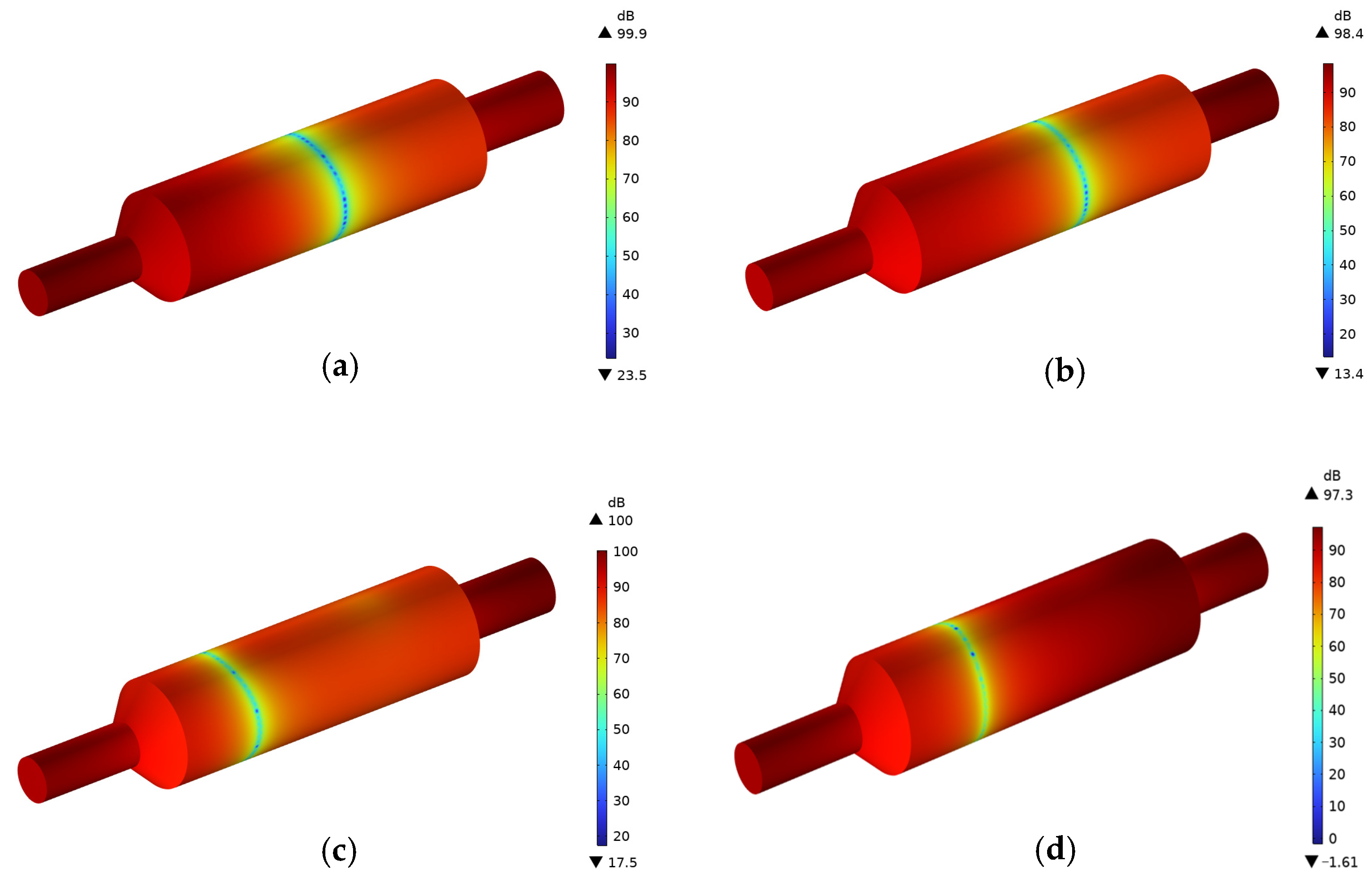
As shown in Table 6, the variation trend of transmission loss considering sound–structure coupling effects at 3500 Hz deviates from that observed at other frequencies. In contrast to the scenario neglecting sound–structure coupling effects, its peak not only undergoes a shift towards lower frequencies, diminishing from 3510 Hz to 3500 Hz, but also exhibits a greater transmission loss. An observation of the sound pressure maps in Figure 18 reveals that at a frequency of 3050 Hz, the peak sound pressure level considering sound–structure coupling effects is lower than the peak sound pressure level neglecting these effects. Conversely, an observation of the sound pressure maps in Figure 19 reveals that the peak sound pressure level considering sound–structure coupling effects (at 3500 Hz) is higher than the peak sound pressure level neglecting these effects (at 3510 Hz). Generally, at specific resonant frequencies, sound–structure coupling effects induce resonance phenomena between the solid structure and acoustic waves, resulting in elevated sound pressure levels, accompanied by an amplified vibration response of the solid structure. This phenomenon consequently influences the acoustic field distribution. Elevated sound pressure results in augmented scattering of acoustic waves at the structural interface, concurrently increasing the reflection efficiency of acoustic waves and thereby leading to an augmentation in transmission loss [33,34]. This elucidates why the transmission loss peak considering sound–structure coupling effects is elevated at a frequency of 3500 Hz.
Table 6.
Comparison of transmission loss formant frequency of the muffler with and without acoustic–structure coupling.
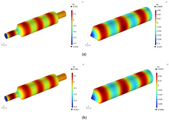
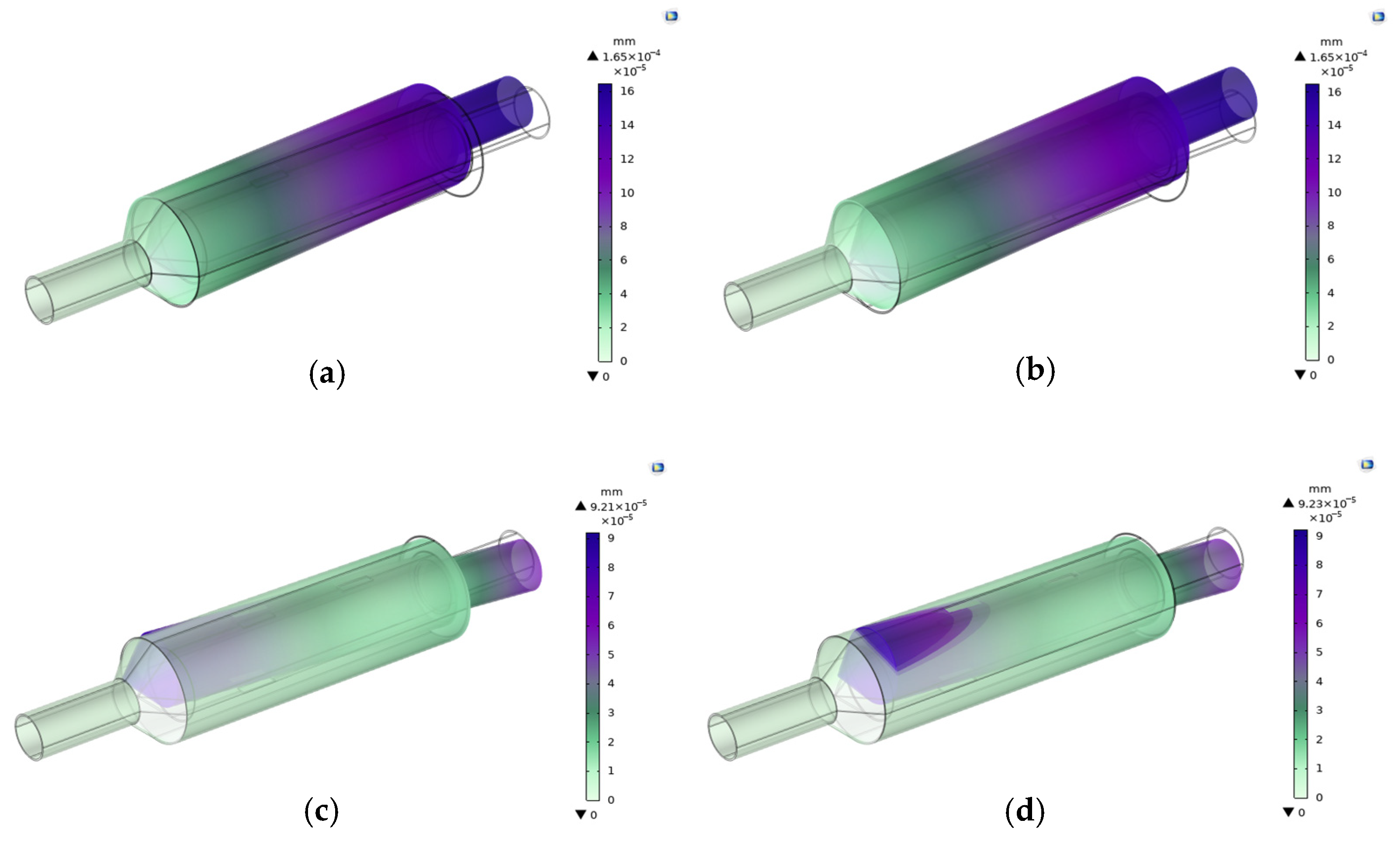
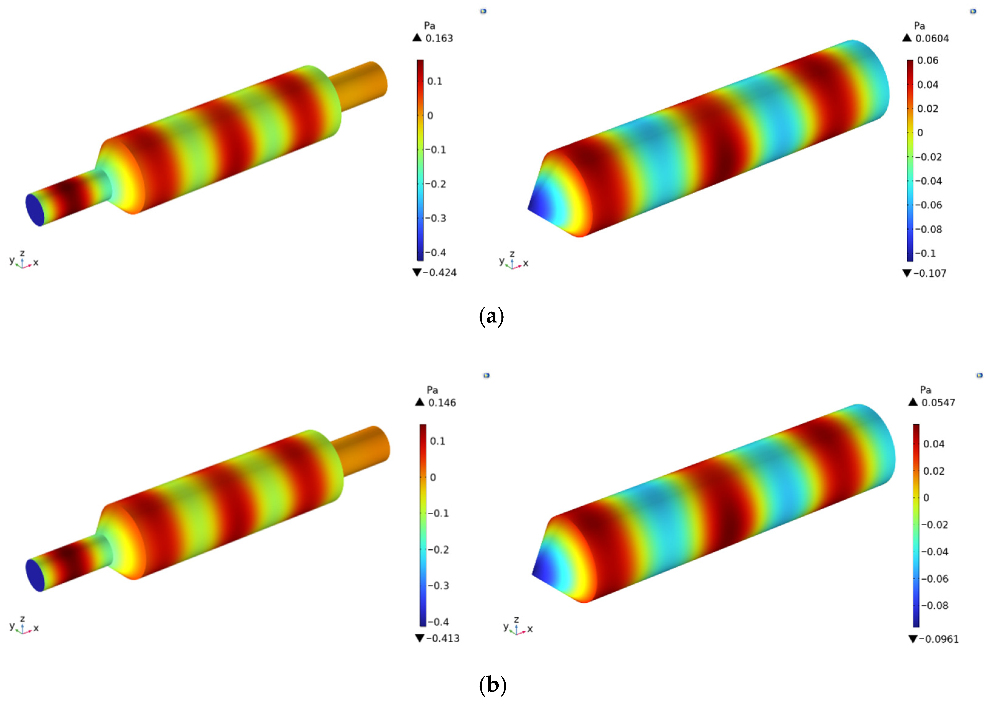
Figure 18.
Frequency–sound pressure graph of the split-stream rushing muffler (1). (a) Without the acoustic–structure coupling effect (3050 Hz), (b) With the acoustic–structure coupling effect (3050 Hz).
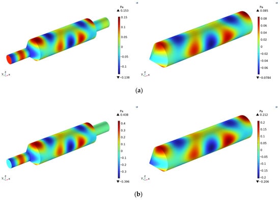
Figure 19.
Frequency–sound pressure graph of the split-stream rushing muffler (2). (a) Without the acoustic–structure coupling effect (3510 Hz), (b) With the acoustic–structure coupling effect (3500 Hz).
6. Single-Factor Influence Analysis and Optimization of the Split-Stream Rushing Exhaust Muffler
6.1. Analysis of the Single-Factor Influence
6.1.1. Wall Thickness
Before performing the single-factor influence analysis on transmission loss considering sound–structure coupling, the value of the muffler wall thickness, a critical structural parameter, must be established. Belonging to the category of thin-walled structures, the muffler features wall thickness as a crucial design parameter. Variations in this parameter not only directly impact the structural rigidity but also exert significant effects on the muffler’s eigenfrequencies and the characteristics of acoustic wave propagation [35]. Typically, augmenting the wall thickness results in an elevation of the muffler’s eigenfrequencies, consequently altering the acoustic field distribution.
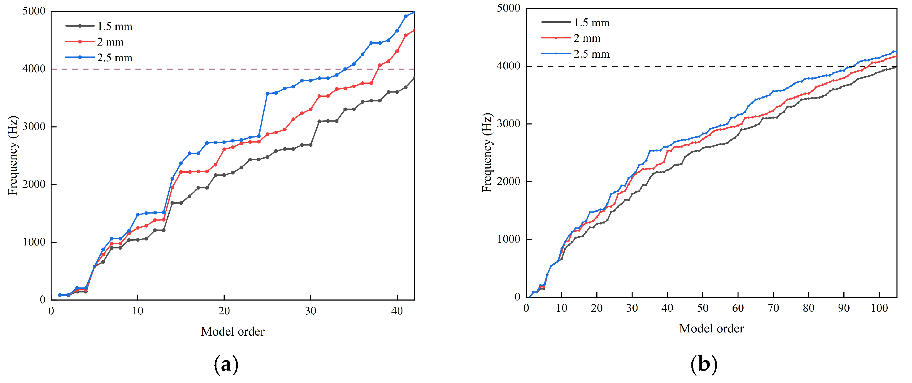
Figure 20 presents a comparative analysis of the eigenfrequencies of structural modes and sound–structure coupled modes concerning their order for three distinct muffler wall thicknesses. Considering that the upper frequency of interest in this study is 4000 Hz, an auxiliary line was incorporated to facilitate analysis. As shown in Figure 20a, the frequency of structural modes of identical order exhibits an upward trend with increasing wall thickness, and the magnitude of the frequency increase also progressively increases with higher modal orders. This indicates that augmenting the wall thickness results in an elevation of the eigenfrequencies for structural modes and sound–structure coupled modes of an identical order.

Figure 20.
Modal frequency diagrams of mufflers with different wall thicknesses. (a) Structural mode, (b) Acoustic–structure coupling.
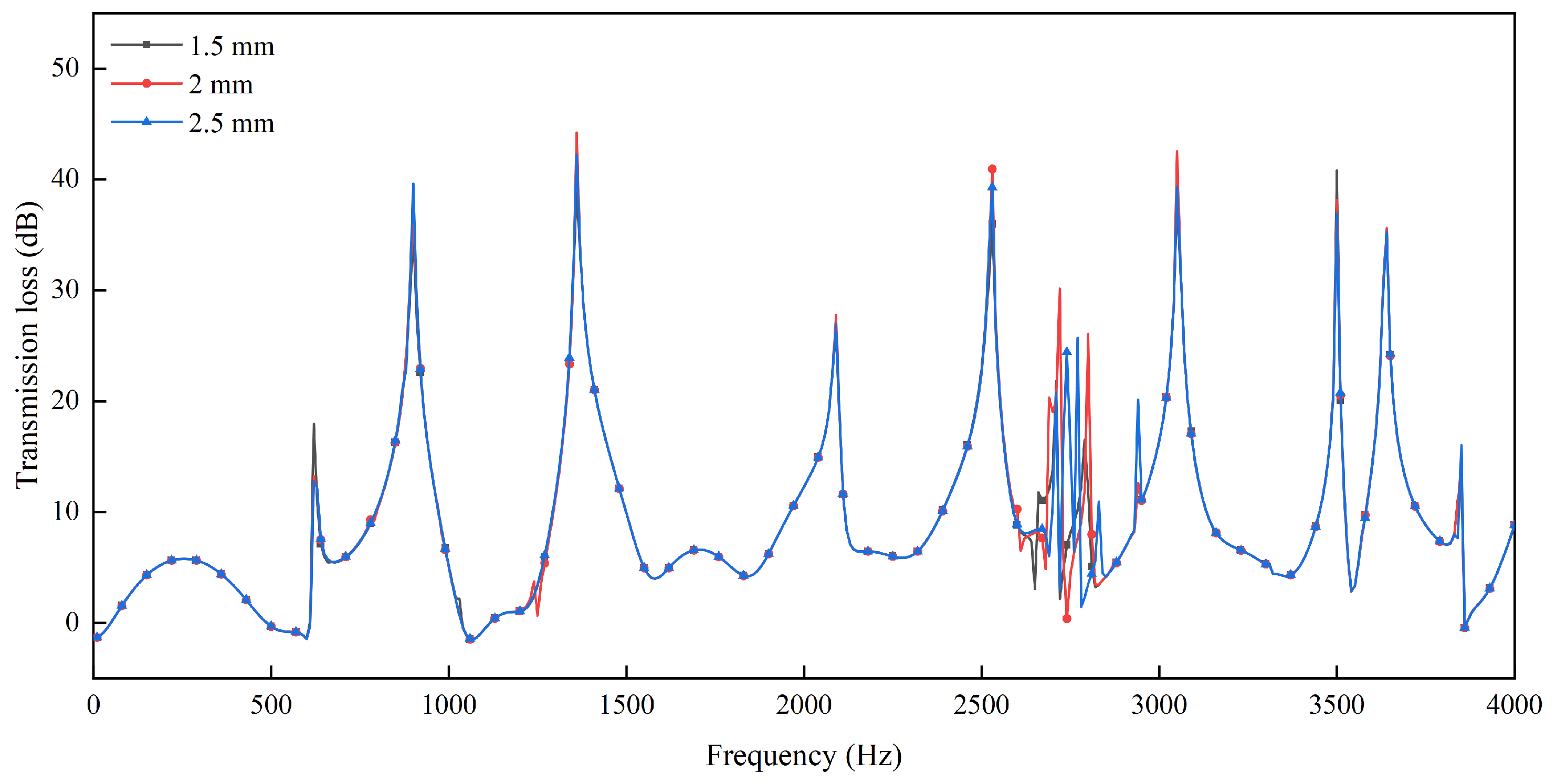
Figure 21 presents the transmission loss characteristics for three distinct wall thicknesses. As shown in Figure 21, variations in wall thickness exert a minimal influence on the transmission loss characteristics of the shunt gas counterflow muffler. The three transmission loss curves exhibit a largely consistent overall trend, with discrepancies primarily localized at the peak values and within certain frequency ranges. This phenomenon indicates that the influence of the wall thickness on transmission loss is contingent upon the synergistic effects of other parameters and does not exhibit a monotonic trend of either an increase or decrease. Considering the peak transmission loss characteristics across varying wall thicknesses, a value of 2 mm was ultimately selected for the muffler wall thickness in the ensuing structural parameter optimization.

Figure 21.
Transmission loss curves for different wall thicknesses under acoustic–structural coupling.
6.1.2. Inner Tube Diameter
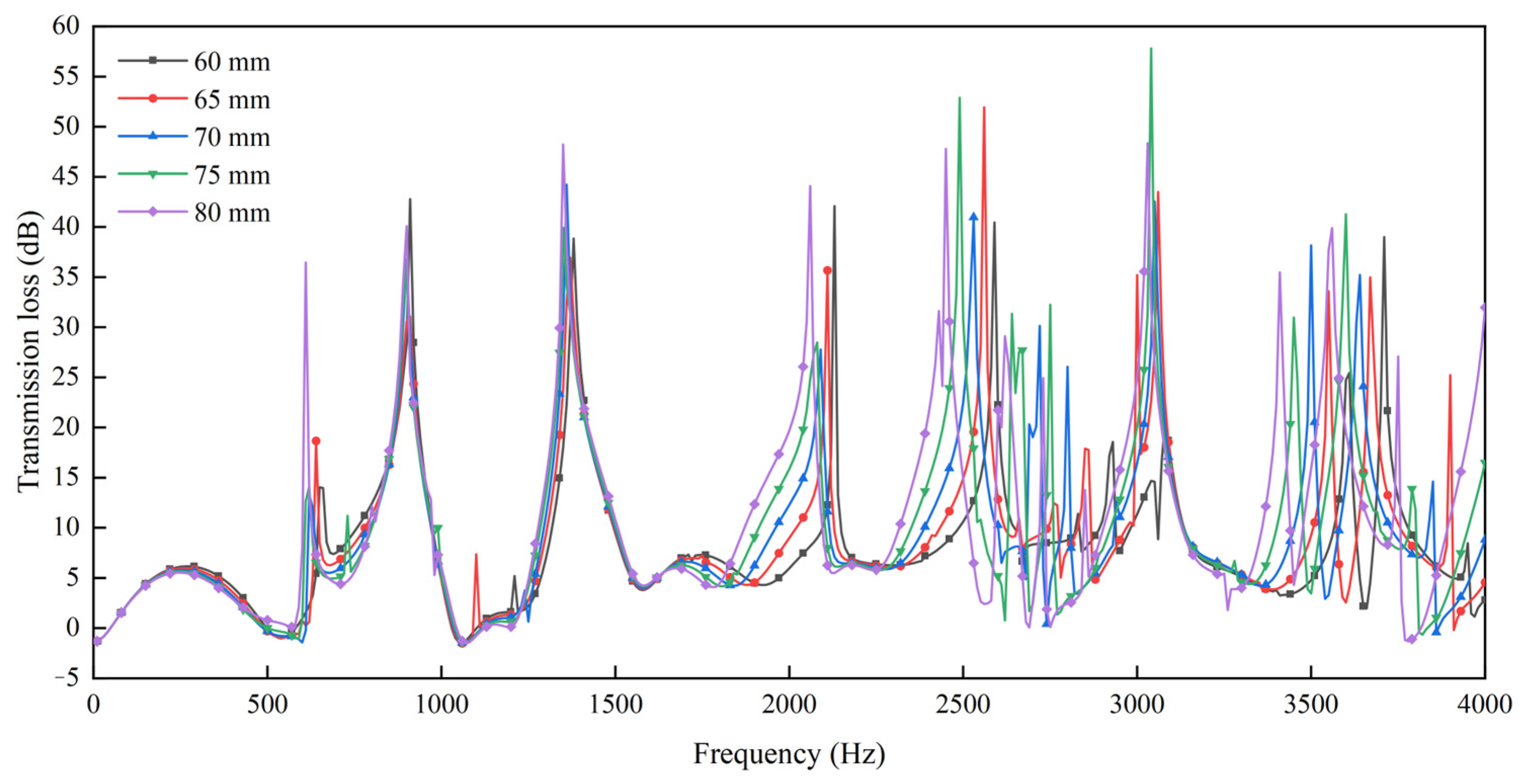
Figure 22 illustrates the annular space defined by the inner and outer pipes of the muffler. The figure illustrates that given constant values for other parameters, the inner pipe diameter determines the dimensions of the annular space, and these dimensions directly influence the acoustic wave propagation characteristics within the muffler. Figure 23 presents the transmission loss characteristics under sound–structure coupling for varying inner pipe diameters while maintaining constant values for the other parameters. An observation of the figure reveals that within the 10–1690 Hz frequency band, the transmission loss exhibits minimal variation. A notable exception occurs at 710 Hz, where the transmission loss increases inversely with the inner pipe diameter. Within the 1690–4000 Hz frequency band, the transmission loss exhibits an overall upward trend with increasing inner pipe diameters. To facilitate further analysis, Table 7 presents the mean transmission loss values for varying inner pipe diameters. As shown in Table 7, the mean transmission loss escalates with increasing inner pipe diameters, and this escalation is substantial, signifying that the inner pipe diameter exerts a considerable influence on the transmission loss under sound–structure coupling.
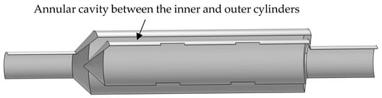
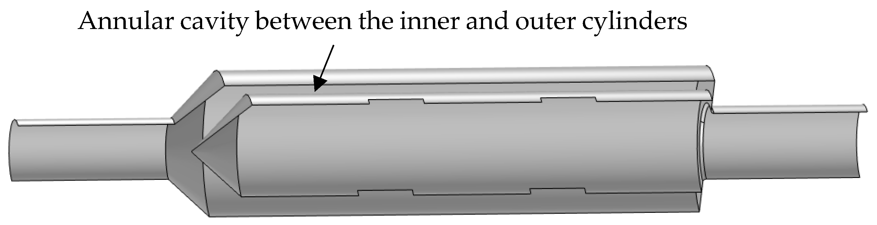
Figure 22.
Schematic diagram of the annular cavity of the muffler (cross-section).

Figure 23.
Comparison of transmission loss for different inner tube diameters under acoustic–structural coupling.
Table 7.
Mean transmission loss for different inner tube diameters under acoustic–structural coupling.
6.1.3. Inner Tube Length
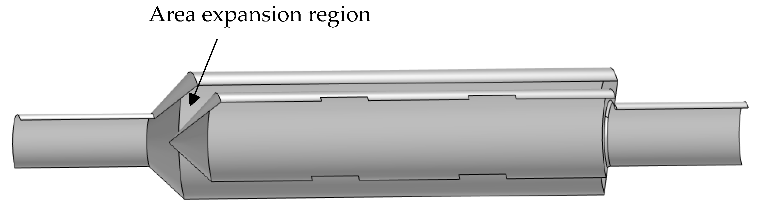
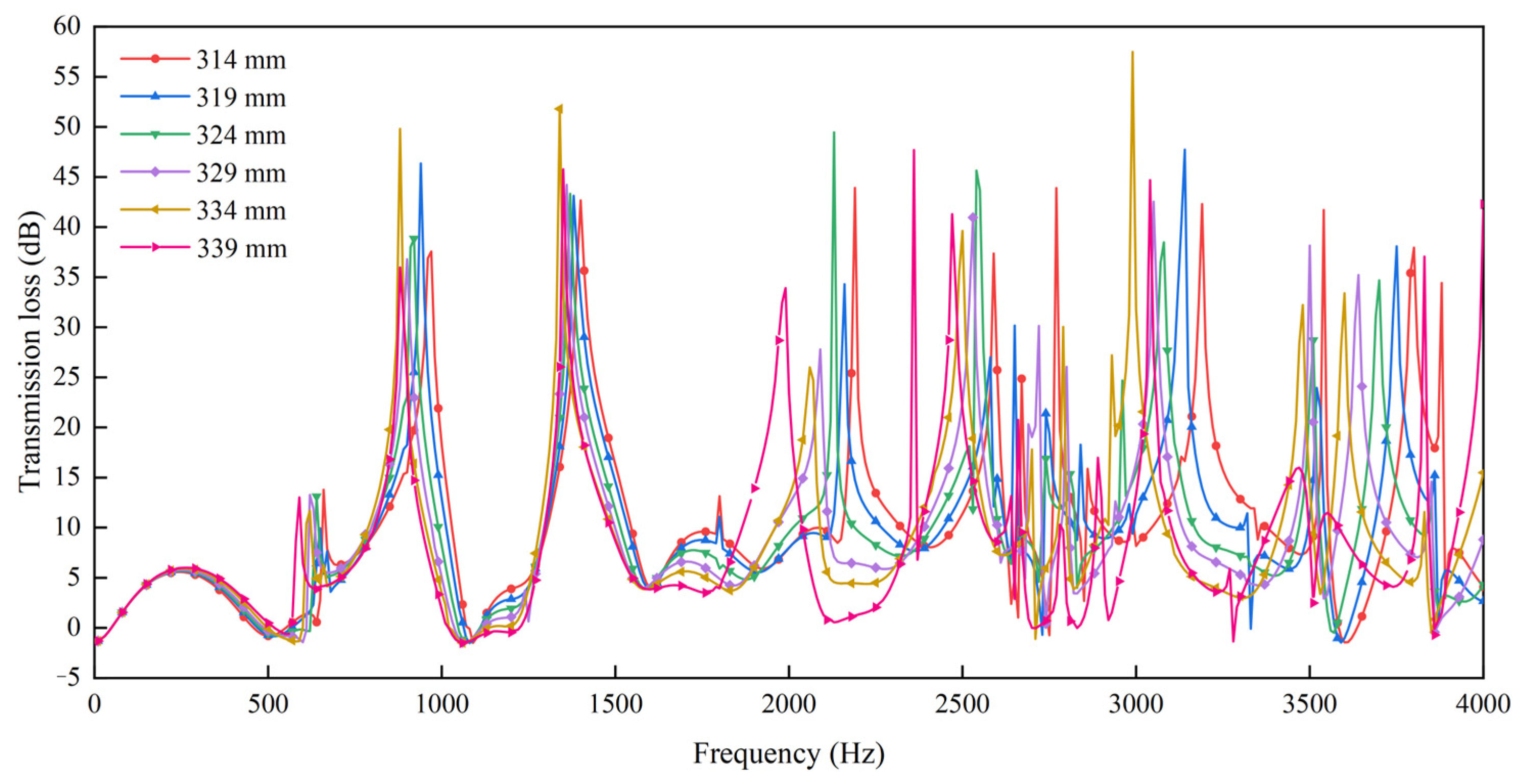
Figure 24 presents a schematic illustration of the diverging section of the conical space defined by the inner and outer pipes of the muffler. Figure 24 illustrates that given constant values for other parameters, the inner pipe length modifies the dimensions of the conical annular space formed by the inner and outer pipes, consequently influencing the acoustic wave propagation characteristics of the muffler. Figure 25 presents the transmission loss characteristics under sound–structure coupling for varying inner pipe lengths. An observation of the figure reveals that the inner pipe length exerts a moderately significant influence on the transmission loss characteristics. Throughout the entire frequency band, the transmission loss curves exhibit an overall downward trend with increasing inner pipe length. To facilitate further analysis, Table 8 presents the mean transmission loss values for varying inner pipe lengths. An observation of the table reveals that the maximum mean transmission loss occurs at an inner pipe length of 314 mm, exceeding the value at 339 mm by 2.02 dB. This discrepancy is moderately substantial, signifying that the inner pipe length exerts a considerable influence on the transmission loss under sound–structure coupling.

Figure 24.
Schematic of the region between the inner and outer conical cavities of the muffler (cross-section).
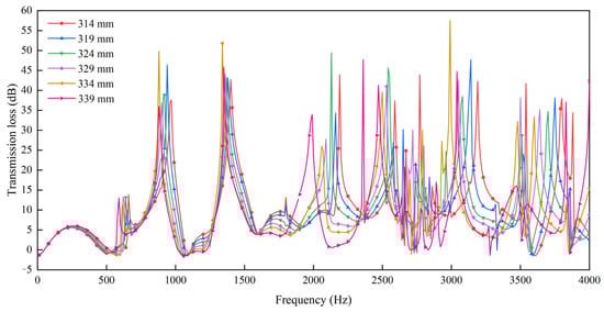
Figure 25.
Comparison of transmission loss for different inner tube lengths under acoustic–structural coupling.
Table 8.
Mean transmission loss for different inner tube lengths under acoustic–structural coupling.
6.2. Optimization Results and Verification
Having analyzed the impacts of three distinct parameters on the split-stream rushing muffler in the preceding section, this section will proceed to optimize its performance predicated on the aforementioned findings. Based on the impacts of the three structural parameters on the transmission loss of the split-stream rushing muffler discussed in the preceding section, the optimized structural parameters are determined as a wall thickness of 2 mm, an inner pipe diameter of 80 mm, and an inner pipe length of 314 mm. The model was built according to the optimized structural parameters of the split-stream rushing muffler to analyze the transmission loss under acoustic–structural coupling conditions, as shown in Figure 26. The mean transmission loss values are presented in Table 9.
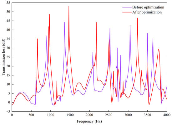
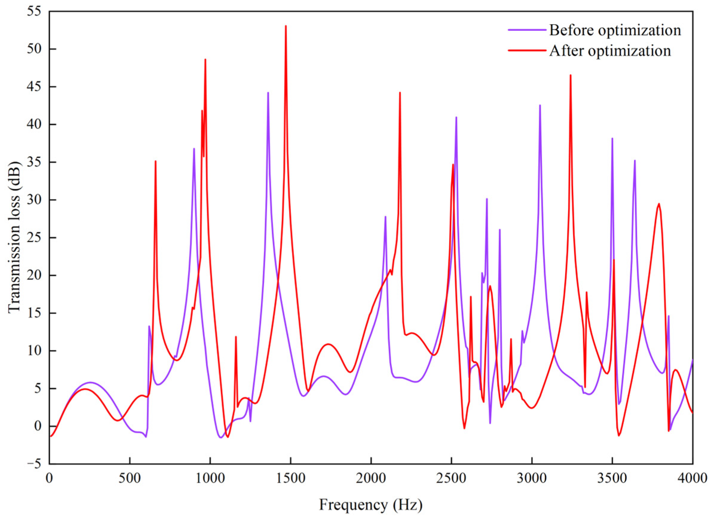
Figure 26.
Transmission loss of the muffler before and after optimization under acoustic–structure coupling.
Table 9.
Mean transmission loss of the muffler before and after optimization under acoustic–structure coupling.
As shown in Figure 26, the muffler with optimized parameters exhibits superior transmission loss characteristics under sound–structure coupling compared to its pre-optimized state across the majority of the frequency spectrum, signifying a favorable optimization outcome. An observation of Table 9 reveals that the mean transmission loss of the optimized muffler considering sound-structure coupling is 11.78 dB. In comparison to the transmission loss level before optimization, the mean transmission loss of the optimized muffler exhibited a 29.5% enhancement, further substantiating the favorable optimization outcome.
7. Conclusions
This study focuses on a split-stream rushing exhaust muffler as its subject of investigation, employing numerical simulation and experimental testing methodologies to examine the sound attenuation performance of the muffler while considering sound–structure coupling effects, and its structural parameters underwent optimization informed by the findings of the single-factor investigation into sound–structure coupling. The main conclusions are as follows:
- (1)
- The muffler underwent structural modal, acoustic cavity modal, and sound–structure coupled modal analyses using the finite element method, and the transmission loss under sound–structure coupling conditions was computed. The findings indicate that novel coupled modes arise from the frequency hybridization and interaction between the structural modes and acoustic cavity modes. The sound–structure coupling effect results in a reduction of the transmission loss peaks across the majority of the frequency spectrum, with a notable exception at 3500 Hz, where the transmission loss exhibits a substantial increase. The findings indicate that this phenomenon stems from the resonance occurring between the solid structure and acoustic wave induced by the sound–structure coupling effect at this specific frequency. The phenomenon of resonance causes an amplification of sound pressure levels, consequently augmenting the scattering of acoustic waves at the structural surface and elevating the reflection coefficient of acoustic waves, culminating in an augmented transmission loss.
- (2)
- A two-load test of the split-stream rushing muffler was conducted. The findings indicate that the transmission loss analysis incorporating sound–structure coupling effects aligns more closely with actual conditions, thereby validating the accuracy and reliability of the simulation model.
- (3)
- The impacts of the wall thickness, inner pipe diameter, and inner pipe length on the acoustic performance of the muffler, considering sound–structure coupling effects, was investigated by employing the single-factor experimental methodology. The findings indicate that the wall thickness exhibits a negligible influence. The inner pipe diameter exhibits a relatively significant influence, with transmission loss escalating in correlation with an increase in diameter. The effect of the inner pipe length on transmission loss is characterized by a downward shift in the frequency spectrum of transmission loss and a reduction in its mean value with increasing inner pipe length. Subsequently, the structural parameters of the muffler underwent optimization. Numerical computations indicate that the optimization outcomes are favorable.
Author Contributions
Conceptualization, P.H. and P.W.; methodology, P.H.; software, P.H. and Y.G.; validation, P.H. and P.W.; formal analysis, P.H.; investigation, P.H.; resources, P.W. and H.S.; data curation, P.H., H.Z., J.X. and Y.Z.; writing—original draft preparation, P.H.; writing—review and editing, P.H. and P.W.; visualization, P.H.; supervision, P.W.; project administration, P.W.; funding acquisition, P.W. and H.S. All authors have read and agreed to the published version of the manuscript.
Funding
This research was funded by the Natural Science Foundation of Inner Mongolia Autonomous Region, grant number 2023MS05022; the Basic Research Fund for Institutions of Inner Mongolia Autonomous Region, grant number BR230155; the Natural Science Foundation of Inner Mongolia Autonomous Region, grant number 2024MS05039; and the Huzhou Natural Science Foundation, grant number 2023YZ01.
Institutional Review Board Statement
Not applicable.
Informed Consent Statement
Not applicable.
Data Availability Statement
The original contributions presented in the study are included in the article.
Acknowledgments
The authors declare that no additional support beyond the listed funding and author contributions was received for this work.
Conflicts of Interest
The authors declare no conflicts of interest.
References
- An Energy Sector Roadmap to Carbon Neutrality in China. Available online: https://iea.blob.core.windows.net/assets/9448bd6e-670e-4cfd-953c-32e822a80f77/AnenergysectorroadmaptocarbonneutralityinChina.pdf (accessed on 1 November 2024).
- Xie, X.Z. Noise optimization design on the exhaust muffler of special vehicle based on the improved genetic algorithm. J. Vibroeng. 2015, 17, 4625–4639. [Google Scholar]
- Shao, Y.L.; Wu, P.; Han, B.S.; Ma, Y.H.; Zhao, Z.W. Acoustic Characteristics of Out-of-Phase and Split-Stream Rushing Muffler for Diesel Engine. Trans. Chin. Soc. Intern. Combust. Engines 2012, 30, 67–71. [Google Scholar]
- Su, H.; Ma, Y.; Wu, P.; Zhang, Y.; Xue, J. Effects of Rushing Hole on Pressure Loss of the Split-Stream-Rushing Muffler Unit. Trans. Chin. Soc. Intern. Combust. Engines 2017, 35, 178–184. [Google Scholar]
- Zhang, Y.; Wu, P.; Ma, Y.; Su, H.; Xue, J. Analysis on acoustic performance and flow field in the split-stream rushing muffler unit. J. Sound. Vib. 2018, 430, 185–195. [Google Scholar] [CrossRef]
- Xue, J.; Zhang, Y.; Su, H.; Wu, P. Study on the acoustic performance of a coupled muffler for diesel engine. Noise Control Eng. J. 2022, 70, 231–245. [Google Scholar] [CrossRef]
- Gladwell, G.M.L.; Zimmermann, G. On energy and complementary energy formulations of acoustic and structural vibration problems. J. Sound Vib. 1966, 3, 233–241. [Google Scholar] [CrossRef]
- Gladwell, G.M.L. A variational formulation of damped acoustic structural vibration problems. J. Sound Vib. 1966, 4, 172–186. [Google Scholar] [CrossRef]
- Nefske, D.J.; Wolf, J.A., Jr.; Howell, L.J. Structural-acoustic finite element analysis of the automobile passenger compartment: A review of current practice. J. Sound Vib. 1982, 80, 247–266. [Google Scholar] [CrossRef]
- Ma, T.F.; Gao, G.; Wang, D.F.; Pan, F. Response Analysis of Interior Structure Noise in Lower Frequency Based on Structure-acoustic Coupling Model. Chin. J. Mech. Eng. 2011, 47, 76–82. [Google Scholar] [CrossRef]
- Ma, T.F.; Ren, C.; Wang, D.F.; Li, W.; Hu, J.H. Experimental Research of Interior Noise Reduction for Passenger Car. Automob. Technol. 2011, 5, 11–15. [Google Scholar]
- Yang, Z.J.; Zhang, J.; Yao, X.G.; Bao, H.P. Study on Acoustic Performance of Exhaust Muffler for Diesel Generator. Mach. Des. Manuf. 2018, 3, 64–66+70. [Google Scholar]
- Xu, J.; Zhang, J.; Ge, J.; Liu, Z. Acoustic-structure coupling analysis and optimization of muffler. IOP Conf. Ser. Mater. Sci. Eng. 2019, 612, 22–23. [Google Scholar] [CrossRef]
- Zhao, B.; Li, H. Analysis of the Influencing Factors of the Acoustic Performance of the Muffler Considering Acoustic-structural Coupling. Arch. Acoust. 2022, 47, 479–490. [Google Scholar]
- Hou, Z.; Si, T.; Zhang, S.; Zhang, Z.; Sun, J. Case study: Analysis of acoustic-structure coupling noise characteristics of the exhaust muffler of an internal combustion engine. Noise Control Eng. J. 2022, 70, 344–363. [Google Scholar] [CrossRef]
- Liu, X.A.; Han, Z.K.; Li, H.; Zhen, R.; Li, L.X. Analysis and optimization of silencing performance of flexible wall expansion muffler. J. Vib. Shock 2023, 42, 142–148. [Google Scholar]
- Nakanishi, E.Y.; Gerges, S.N.Y. Acoustic Modal Analysis for Vehicle Cabin. In SAE Technical Paper 952246; SAE International: Warrendale, PA, USA, 1995; Available online: https://saemobilus.sae.org/papers/acoustic-modal-analysis-vehicle-cabin-952246 (accessed on 21 April 2025).
- Chu, Z.G.; Liu, X.H.; Shen, L.B.; Gao, X.X.; Zhang, J.Y. Effects of Acoustic Modes in Chamber on Acoustic Attenuation Characteristics of Reactive Silencing Elements. Chin. Intern. Combust. Engine Eng. 2016, 37, 147–154. [Google Scholar]
- Tao, L.Y.; Xu, D.G.; Cang, X.G. Analysis of Shell Structural–acoustic Coupling Based on Smoothed Finite Element and Finite Element Method. Chin. J. Mech. Eng. 2010, 21, 1765–1770. [Google Scholar]
- Davidsson, P. Structure-Acoustic Analysis: Finite Element Modeling and Reduction Methods. Doctoral Thesis, Lund University, Lund, Sweden, 2004. [Google Scholar]
- Zhong, J.; Zhao, H.; Yang, H.; Yin, J.; Wen, J. Effect of Poisson’s loss factor of rubbery material on underwater sound absorption of anechoic coatings. J. Sound Vib. 2018, 424, 293–301. [Google Scholar] [CrossRef]
- Middelberg, J.M.; Barber, T.J.; Leong, S.S.; Byrne, K.P.; Leonardi, E. CFD Analysis of the Acoustic and Mean Flow Performance of Simple Expansion Chamber Mufflers. In Proceedings of the IMECE 2004, Anaheim, CA, USA, 13–19 November 2004; pp. 151–156. [Google Scholar]
- Hua, X.; Zhang, Y.; Herrin, D.W. The effect of conical adapters and choice of reference microphone when using the two-load method for measuring muffler transmission loss. Appl. Acoust. 2015, 93, 75–87. [Google Scholar] [CrossRef]
- Xu, H.S.; Kang, Z.X.; Ji, Z.L. Experimental measurement and analysis of transmission loss of exhaust silencers. Noise Vib. Control 2009, 29, 128–131. [Google Scholar]
- ASTM E1050 19; Standard Test Method for Impedance and Absorption of Acoustical Materials Using a Tube, Two Microphones and a Digital Frequency Analysis System. ASTM: West Conshohocken, PA, USA, 2019. Available online: https://cdn.standards.iteh.ai/samples/104506/d21515b4917d4651ad596c484cce53cb/ASTM-E1050-19.pdf (accessed on 19 November 2024).
- ASTM E1050 98; Standard Test Method for Impedance and Absorption of Acoustical Materials Using a Tube, Two Microphones and a Digital Frequency Analysis System. ASTM: West Conshohocken, PA, USA, 1998. Available online: https://cdn.standards.iteh.ai/samples/7786/4759c54bc678469d897dd45607d37c71/ASTM-E1050-98.pdf (accessed on 17 November 2024).
- GB/Z 27764-2011; Acoustics—Determination of Sound Transmission Loss in Impedance Tubes—Transfer Matrix Method. Standardization Administration of China: Beijing, China, 2011. Available online: http://c.gb688.cn/bzgk/gb/showGb?type=online&hcno=0EE9C9EFF301F2F0014C295674E7DAF3 (accessed on 20 November 2024).
- GB/T 4759-2009Exhaust Silencers for Internal Combustion Engines—Measurement Procedure; Standardization Administration of China: Beijing, China, 2009. Available online: https://openstd.samr.gov.cn/bzgk/gb/newGbInfo?hcno=0BDA311249F55E0F7F83C013EB30FA67 (accessed on 21 April 2025).
- Crocker, M.J. Handbook of Acoustics; John Wiley & Sons: Hoboken, NJ, USA, 1998; pp. 1367–1427. [Google Scholar]
- Nayfeh, S.A.; Nayfeh, A.H. Energy transfer from high-to low-frequency modes in a flexible structure via modulation. ASME J. Vib. Acoust. 1994, 116, 203–207. [Google Scholar] [CrossRef]
- Shui, Y.B.; Xu, X.C.; Cao, Z.L. The research on acoustic performance of automotive exhaust muffler based on multi-field coupling. Manuf. Autom. 2015, 37, 67–69. [Google Scholar]
- Gardner, B.; Mejdi, A.; Musser, C.; Chaigne, S.; Macarios, T.D.C. Coupled CFD and Vibro-Acoustic Modeling of Complex-Shaped Mufflers Accounting for Non-Uniform Mean Flow Effects. SAE Tech. Pap. 2015, 1, 2313. [Google Scholar]
- Remington, P.J. Structure-Borne Sound: Structural Vibrations and Sound Radiation at Audio Frequencies. J. Acoust. Soc. Am. 2005, 118, 2754. [Google Scholar] [CrossRef]
- Norton, M.P.; Karczub, D.G. Fundamentals of Noise and Vibration Analysis for Engineers; Cambridge University Press: Cambridge, UK, 2003; pp. 193–250. [Google Scholar]
- Mosa, A.I.; Putra, A.; Mahmood, H.A. Evaluating the impact of structure parameters on the acoustic performance of an exhaust muffler with shells. East. Eur. J. Enterp. Technol. 2023, 126, 33–44. [Google Scholar] [CrossRef]


Disclaimer/Publisher’s Note: The statements, opinions and data contained in all publications are solely those of the individual author(s) and contributor(s) and not of MDPI and/or the editor(s). MDPI and/or the editor(s) disclaim responsibility for any injury to people or property resulting from any ideas, methods, instructions or products referred to in the content. |
© 2025 by the authors. Licensee MDPI, Basel, Switzerland. This article is an open access article distributed under the terms and conditions of the Creative Commons Attribution (CC BY) license (https://creativecommons.org/licenses/by/4.0/).