
Detection of Nutrients and Contaminants in the Agri-Food Industry Evaluating the Probabilities of False Compliance and False Non-Compliance Through PLS Models and NIR Spectroscopy

 , , and
Abstract
:1. Introduction
- Determine the quantity that can be ensured when maximum permitted limits are established by official regulations (as for agrochemicals or prohibited substances) or when minimum or maximum limits are established for a certain parameter in a food matrix by the industry itself to guarantee the quality of their products
- Ascertain with statistical guarantee the minimum amount that it is possible to discriminate in a certain analytical method.
2. Materials and Methods
2.1. Instrumentation and Experimental Methods

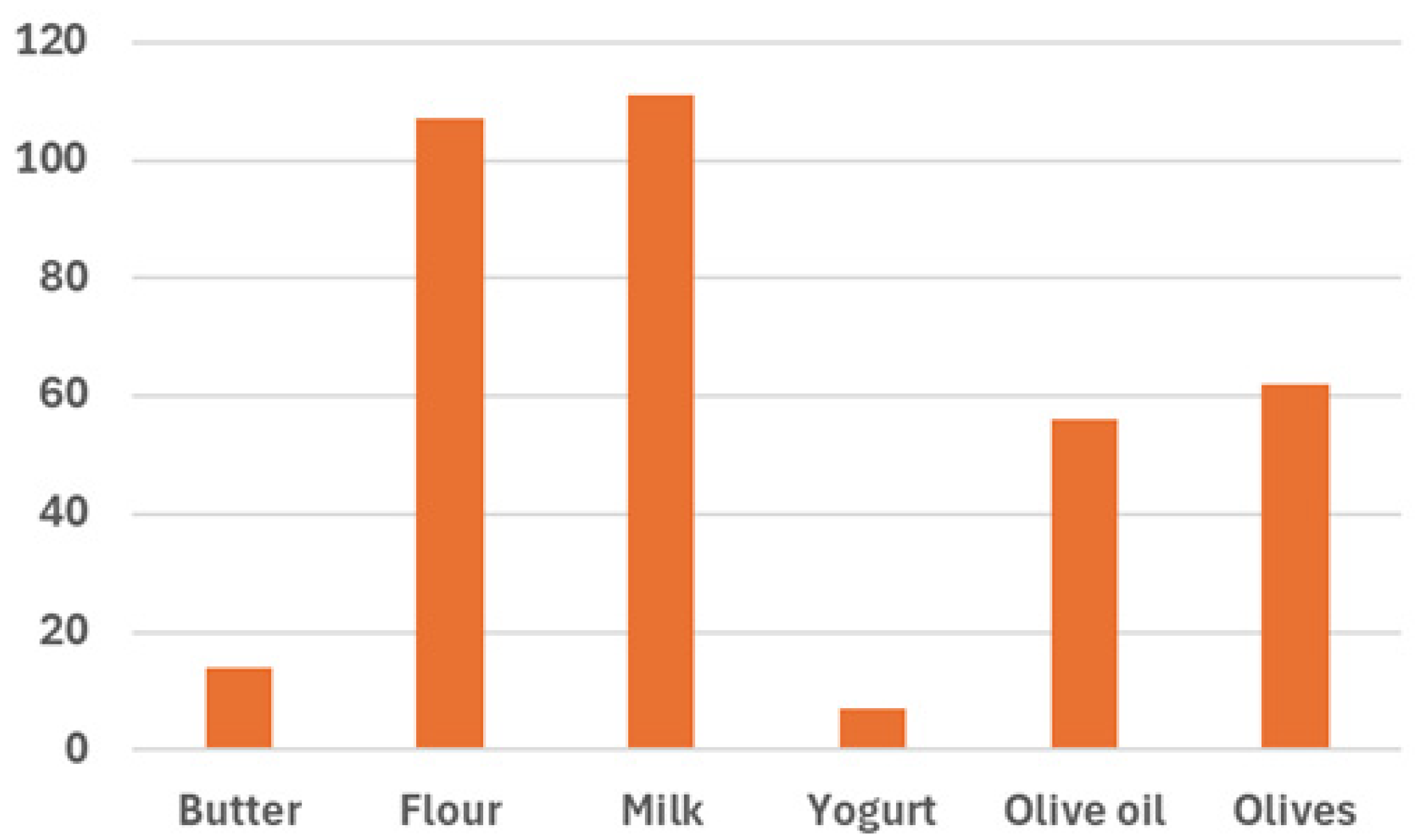
| Matrix | Analyte | Reference Method | N * | Sample Replicates | Spectral Replicates | Final Data Matrix | Data Matrix of the Prediction Set |
|---|---|---|---|---|---|---|---|
| Butter | Fat (%) (w/w) | NMR | 11 | 2 | 3 | 66 × 125 | 24 × 125 |
| Salt (%) (w/w) | Atomic absorption | ||||||
| Flour | Protein (%) (w/w) | Kjeldahl method | 36 | 3 | 3 or 6 | 504 × 125 | - |
| Milk | Fat (%) (w/w) | FTIR | 38 | 1 or 2 | 3 | 195 × 125 | 52 × 125 |
| Protein (%) (w/w) | FTIR | ||||||
| Yogurt | Fat (%) (w/w) | Gravimetry | 19 | 2 or 4 | 3 | 144 × 125 | 24 × 125 |
| Protein (%) (w/w) | Kjeldahl method | ||||||
| Olive oil | Refined olive oil (%) (v/v) | ** | 14 | 1 or 2 | 3 | 81 × 125 | 18 × 125 |
| Olives | Both agrochemicals (mg kg−1) | GC-MS-MS QqQ | 40 | 1 | *** | 40 × 125 | - |
2.2. Statistical Method
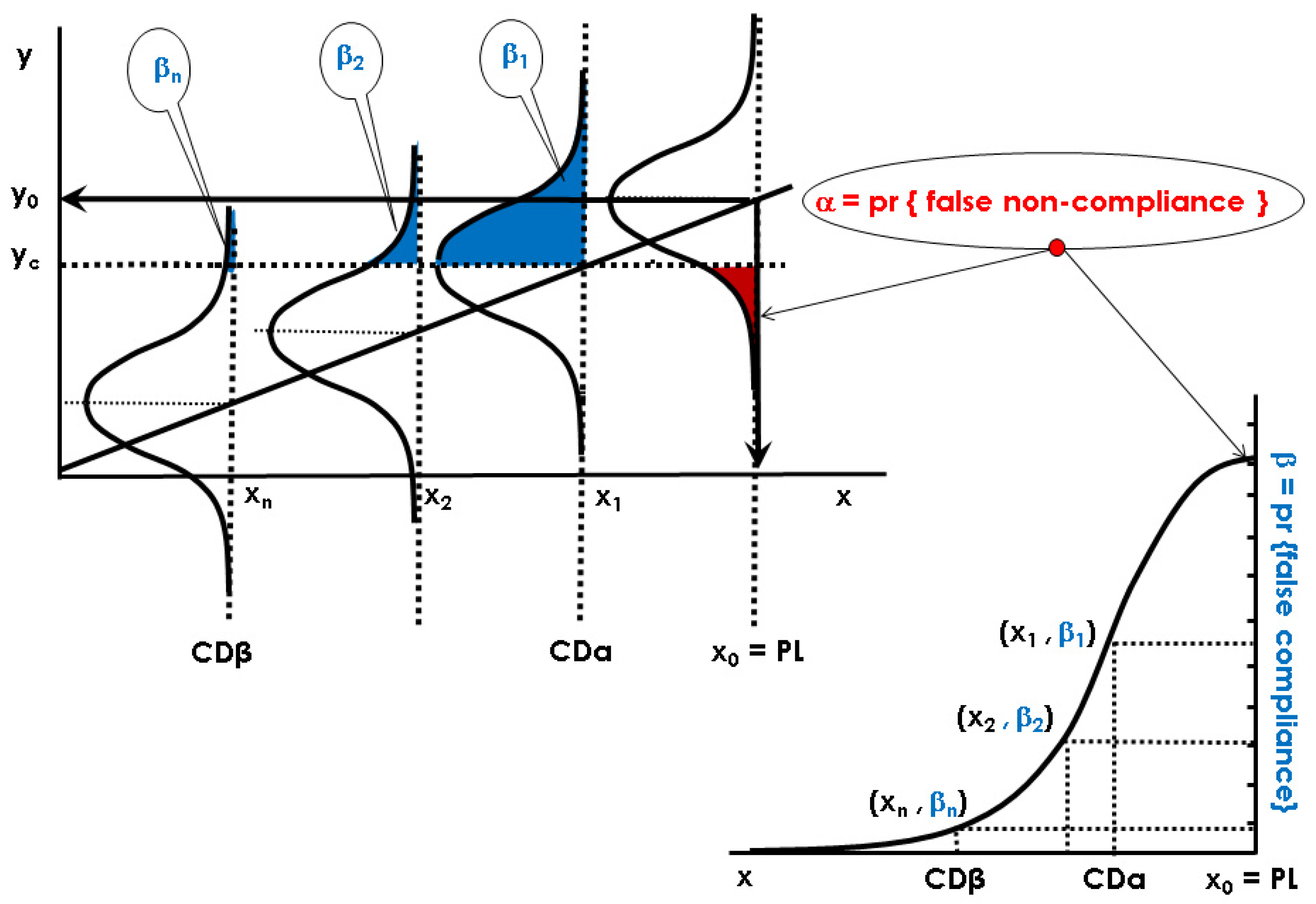
2.2.1. Decision Limit and Capability of Detection at x0 = 0 or for a Permitted Limit, x0 = PL with Multivariate Signals
Ha: x < x0 (the parameter is less than x0, non-compliant sample)
Ha: x > x0 (the parameter is greater than x0, non-compliant sample)
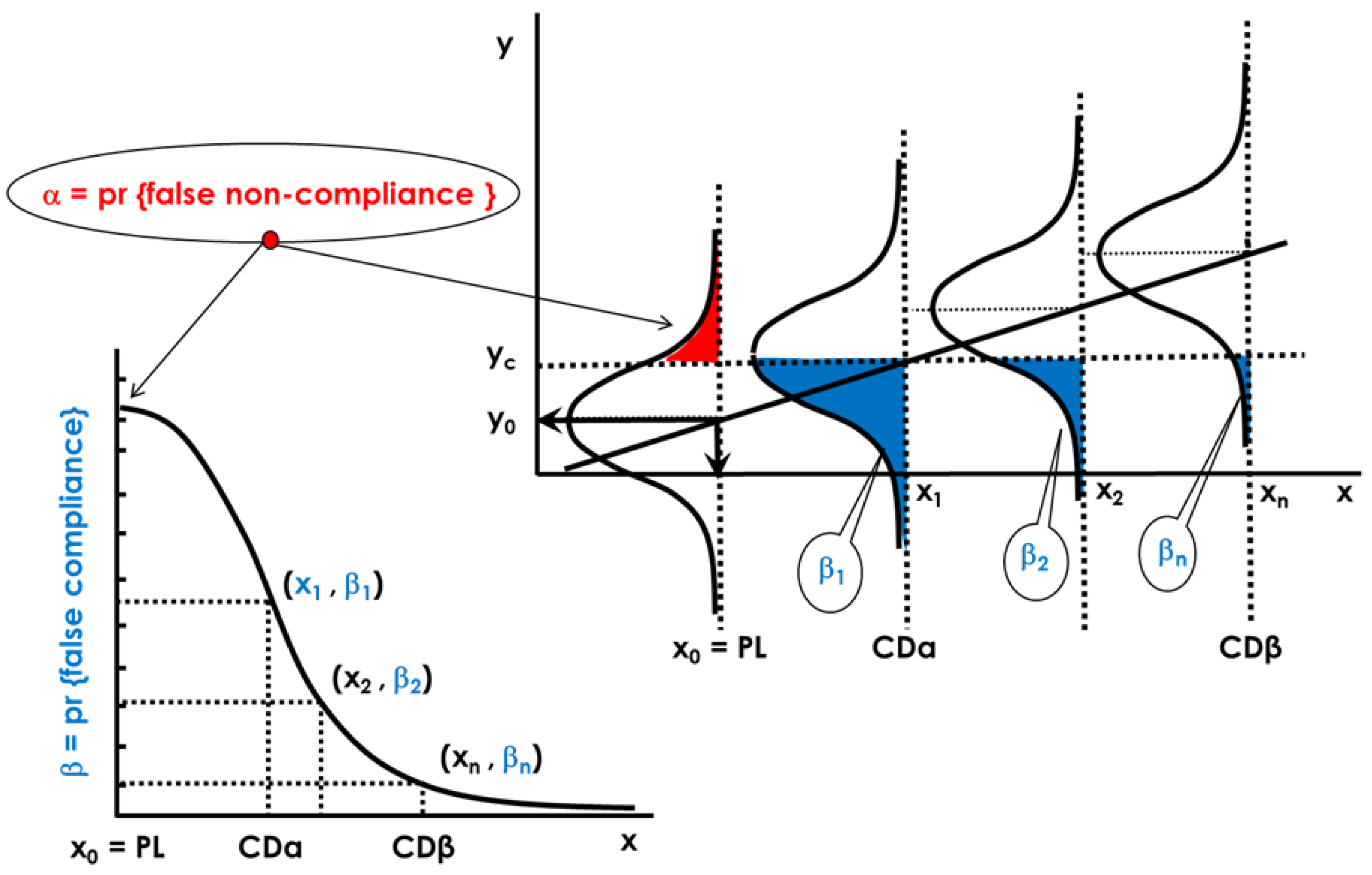
2.2.2. Capability of Discrimination or Multivariate Sensitivity
Ha: x ≠ x0 (the parameter is smaller or greater than x0, non-compliant sample)
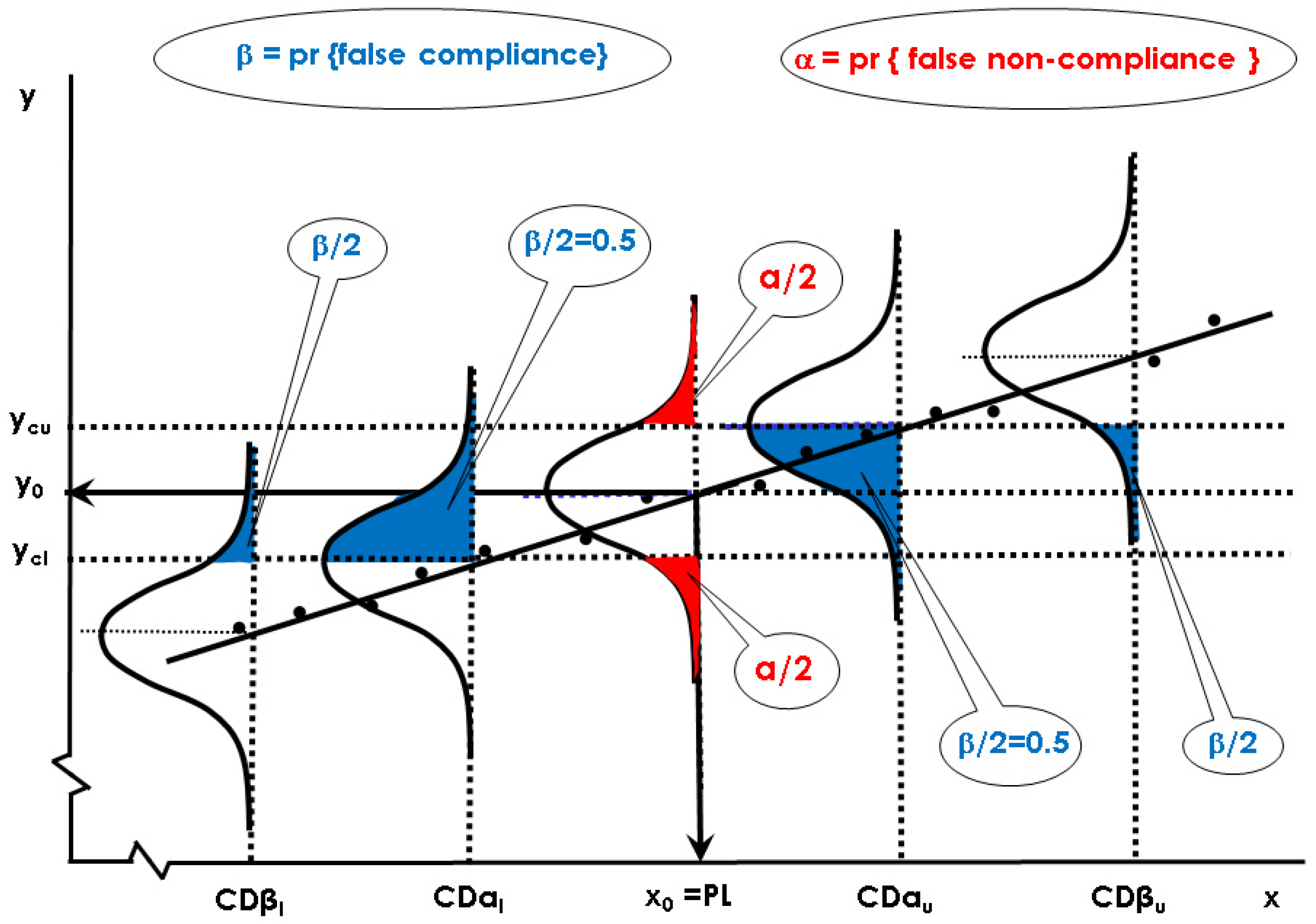
2.2.3. Global Procedure for Multivariate Calibration to Guarantee CCα and CCβ (or CDα and CDβ) with NIR Spectroscopy and a PLS Model
- To build a PLS model for each parameter, y = f(X), (i) first, the predictors were preprocessed by applying the standard normal variate (SNV) followed by a first (D1) or a second (D2) derivative and a second-degree polynomial (also varying the window size from 9 and 15) depending on the case of study. Then, both the predictors and the responses were mean-centered (all the details can be consulted for each data set and each case in Table 2). (ii) The number of latent variables was selected through cross validation. (iii) The samples with a standardized residue greater than 3 (in the absolute value) or with both Q residuals and T2 Hotelling values larger than their corresponding threshold values at a 95% confidence level were removed (outliers). (iv) Steps (ii) and (iii) were repeated until no outliers were detected;
- The accuracy line was then built by means of a least squares regression, representing the predicted values obtained with the PLS models (y) versus the true concentration (x) obtained using the reference method specified in Table 1 for each case of study. In this way, the predicted and true concentrations are linked by means of a linear model. The characteristics of every constructed accuracy line can be found in Table 3, whereas their graphical representations can be seen in Figure S1 in the Supplementary Material;
- Using the data resulting from the accuracy lines, CCα and CCβ (or CDα and CDβ) were calculated for probabilities of both a false positive and false negative (or false non-compliance and false compliance) of 0.05, regarding the definitions in Section 2.2.1 and Section 2.2.2.
- The final results, after applying this global procedure, can be consulted in Section 3.
3. Results
3.1. PLS Calibration
| Matrix | Analyte | Preprocess 1 | LV | Variance of x-Block (%) | Variance of y-Block (%) | Out. 2 | RMSEC | RMSECV | RMSEP |
|---|---|---|---|---|---|---|---|---|---|
| Butter | Fat (%) | SNV + 1D (2, 11) + MC | 4 | 94.98 | 95.10 | - | 0.295 | 0.437 | 0.317 |
| Salt (%) | SNV + 1D (2, 11) + MC | 6 | 98.68 | 96.46 | - | 0.084 | 0.175 | 0.175 | |
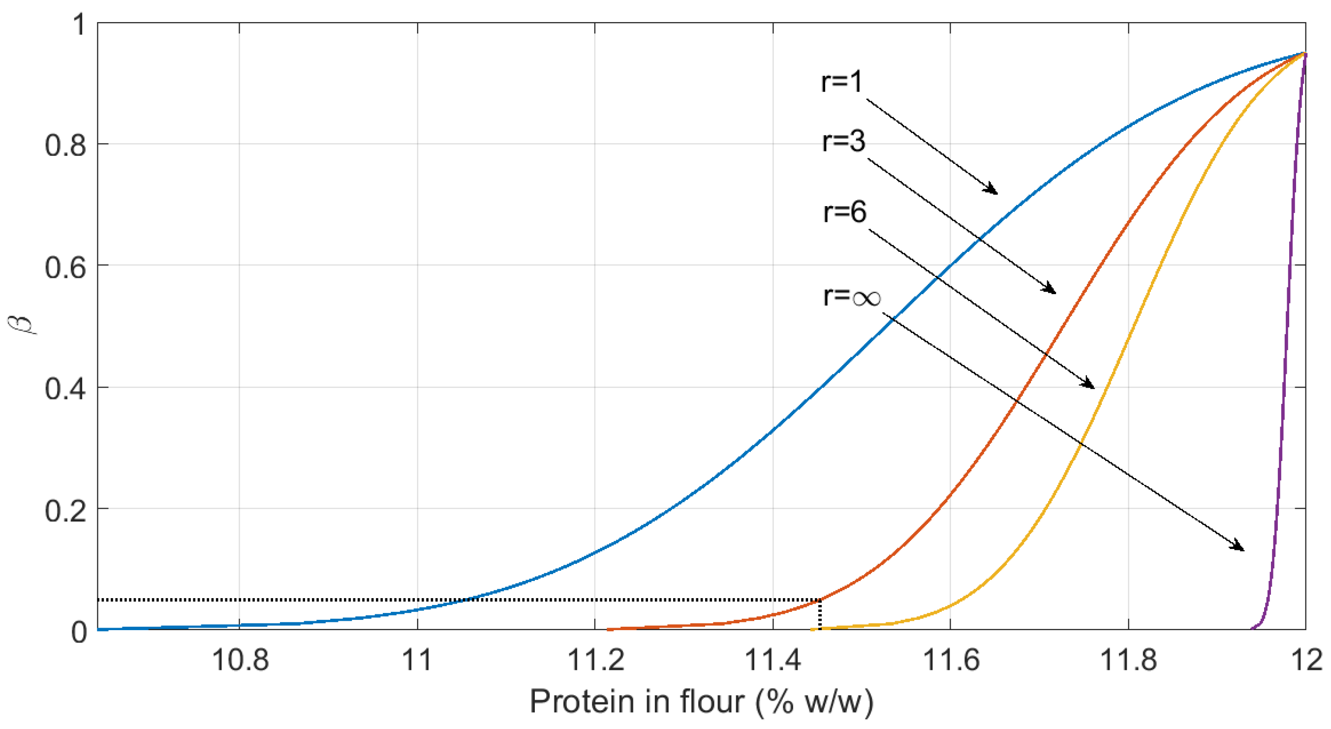
| Flour | Protein (%) | SNV + 2D (2, 13) + MC | 7 | 97.00 | 95.15 | 20 | 0.278 | 0.357 | - |
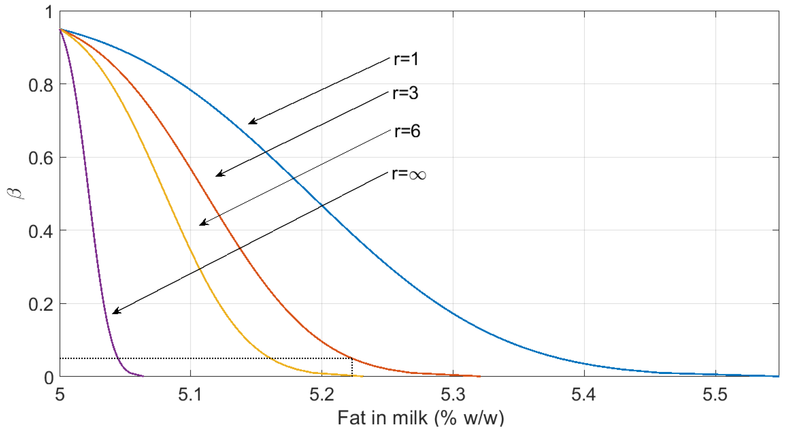
| Milk | Fat (%) | SNV + 2D (2, 13) + MC | 6 | 98.32 | 96.11 | 3 | 0.112 | 0.135 | 0.172 |
| Protein (%) | SNV + 2D (2, 13) + MC | 4 | 96.77 | 90.32 | 6 | 0.105 | 0.117 | 0.085 | |
| Yogurt | Fat (%) | SNV + 2D (2, 9) + MC | 6 | 99.31 | 98.60 | 7 | 0.292 | 0.360 | 0.315 |
| Protein (%) | SNV + MC | 7 | 99.95 | 96.40 | 2 | 0.177 | 0.207 | 0.215 | |
| Olive oil | Refined olive oil (%) | SNV + 2D (2, 15) + MC | 4 | 94.99 | 94.13 | 5 | 2.896 | 3.620 | 2.872 |
| Olives | Diflufenican (mg kg−1) | SNV + 2D (2, 7) + MC | 7 | 97.09 | 94.90 | 2 | 0.317 | 0.484 | - |
| Piretrin (mg kg−1) | SNV + 2D (2, 7) + MC | 7 | 92.09 | 95.93 | - | 0.971 | 1.644 | - |
| Matrix | Analyte | N | Analyte Range | Intercept | Slope | syx | p-Value * | |
|---|---|---|---|---|---|---|---|---|
| Min | Max | |||||||
| Butter | Fat (%) | 66 | 81.10 | 86.60 | 4.109 | 0.951 | 0.293 | <0.0001 |
| Salt (%) | 66 | 0.00 | 1.20 | 0.008 | 0.965 | 0.083 | <0.0001 | |
| Flour | Protein (%) | 484 | 9.41 | 14.58 | 0.575 | 0.952 | 0.272 | <0.0001 |
| Milk | Fat (%) | 192 | 3.65 | 6.16 | 0.166 | 0.961 | 0.110 | 0.0058 |
| Protein (%) | 190 | 3.09 | 4.27 | 0.339 | 0.904 | 0.100 | <0.0001 | |
| Yogurt | Fat (%) | 137 | 0.1 | 9.4 | 0.038 | 0.986 | 0.292 | <0.0001 |
| Protein (%) | 142 | 2.8 | 6.4 | 0.137 | 0.964 | 0.174 | <0.0001 | |
| Olive oil | Refined olive oil (%) | 76 | 61 | 100 | 4.794 | 0.941 | 2.847 | <0.0001 |
| Olives | Diflufenican (mg kg−1) | 38 | 0.00 | 3.42 | 0.047 | 0.949 | 0.281 | <0.0001 |
| Piretrin (mg kg−1) | 40 | 0.00 | 11.40 | 0.126 | 0.9593 | 0.869 | <0.0001 | |
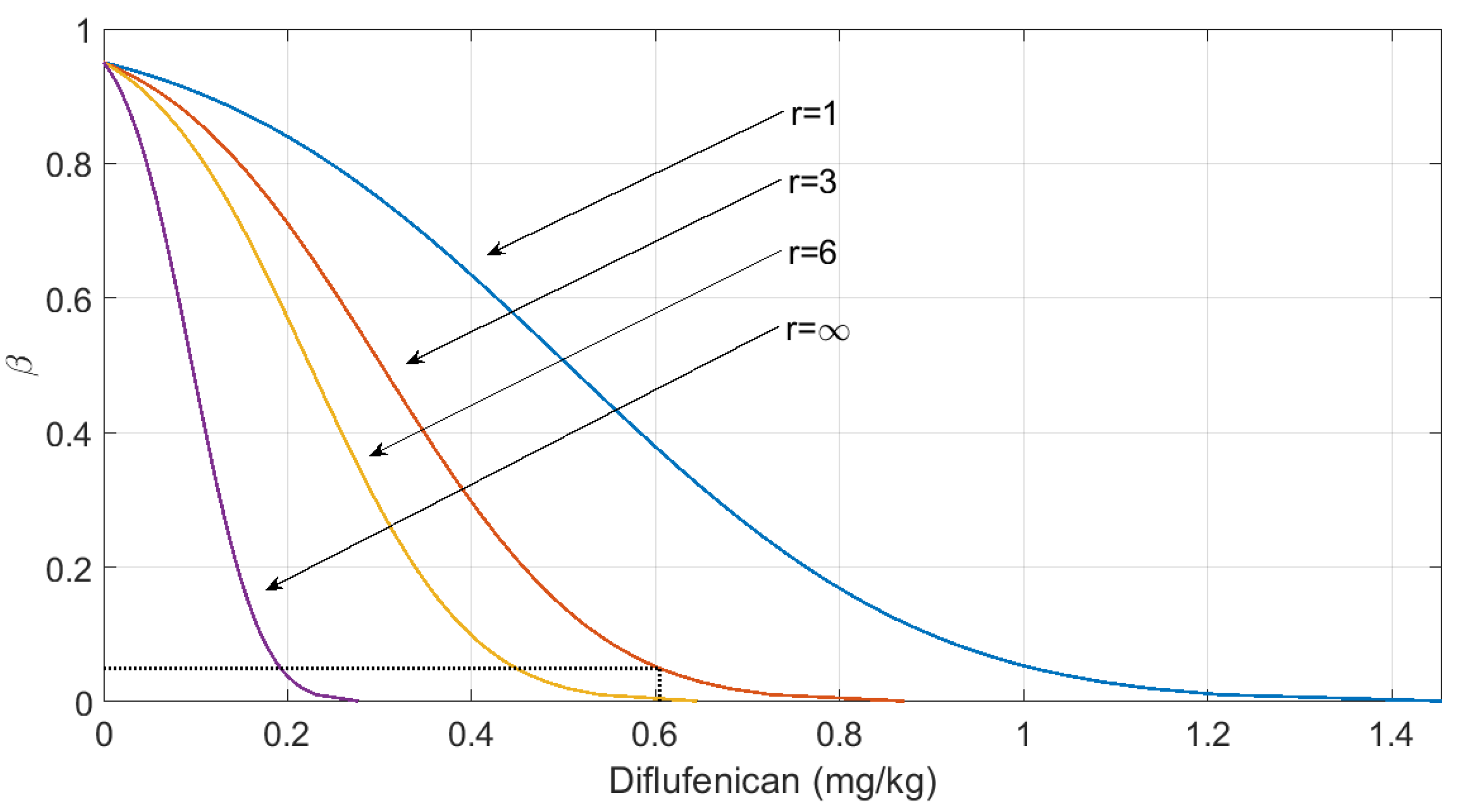
3.2. Estimation of the Capability of Detection and the Capability of Discrimination

| Matrix | Analyte | N | Range | PL = x0 | yc | CCα | CCβ | CDα | CDβ | |
|---|---|---|---|---|---|---|---|---|---|---|
| Min | Max | |||||||||
| Butter | Fat (%) | 66 | 81.10 | 86.60 | 85 * | 84.94/85.64 | - | - | [84.63, 85.36] | [84.27, 85.73] |
| Salt (%) | 66 | 0.00 | 1.20 | 0 | 0.091 | 0.086 | 0.171 | - | - | |
| 1.2 ** | 1.077 | - | - | 1.11 | 1.02 | |||||
| Flour | Protein (%) | 484 | 9.41 | 14.58 | 12 ** | 11.733 | - | - | 11.73 | 11.45 |
| Milk | Fat (%) | 192 | 3.65 | 6.16 | 5 *** | 5.079 | - | - | 5.11 | 5.22 |
| Protein (%) | 190 | 3.09 | 4.27 | 4 ** | 3.856 | - | - | 3.89 | 3.78 | |
| Yogurt | Fat (%) | 137 | 0.1 | 9.4 | 0 | 0.322 | 0.290 | 0.580 | - | - |
| Protein (%) | 142 | 2.8 | 6.4 | 3 ** | 2.867 | - | - | 2.83 | 2.65 | |
| Olive oil | Refined olive oil (%) | 76 | 61 | 100 | 80 ** | 77.30 | - | - | 77.03 | 74.07 |
| Olives | Diflufenican (mg kg−1) | 38 | 0.00 | 3.42 | 0 | 0.336 | 0.304 | 0.604 | - | - |
| 0.6 *** | 0.901 | - | - | 0.90 | 1.20 | |||||
| Piretrin (mg kg−1) | 40 | 0.00 | 11.40 | 0 | 1.016 | 0.928 | 1.844 | - | - | |
| 0.5 *** | 1.492 | - | - | 1.42 | 2.34 | |||||
4. Discussion
4.1. Contributions and Practical Implications
4.2. Directions of Future Research
Supplementary Materials
Author Contributions
Funding
Institutional Review Board Statement
Informed Consent Statement
Data Availability Statement
Acknowledgments
Conflicts of Interest
Abbreviations
| NIR | Near infrared |
| PLS | Partial Least Squares |
| ISO | International Organization for Standardization |
| MIR | Medium infrared |
| IUPAC | International Union of Pure and Applied Chemistry |
| NMR | Nuclear magnetic resonance |
| FTIR | Fourier transform infrared |
| GC-MS-MS | Gas chromatography coupled to mass spectrometry |
| QqQ | Triple quadrupole |
| PL | Permitted limit/established limit |
| SNV | Standard normal variate |
| LV | Latent variable |
| CCα | Decision limit |
| CCβ | Capability of detection |
| CDα | Decision limit for a permitted limit different from 0 |
| CDβ | Capability of discrimination for a permitted limit different from 0 |
References
- FDA Releases New Food Fraud Webpage. Available online: https://www.food-safety.com/articles/7424-fda-releases-new-food-fraud-webpage (accessed on 16 April 2025).
- Choudhary, A.; Gupta, N.; Hameed, F.; Choton, S. An Overview of Food Adulteration: Concept, Sources, Impact, Challenges and Detection. Int. J. Chem. Stud. 2020, 8, 2564–2573. [Google Scholar] [CrossRef]
- Casarin, P.; Giopato Viell, F.L.; Good Kitzberger, C.S.; dos Santos, L.D.; Melquiades, F.; Bona, E. Determination of the Proximate Composition and Detection of Adulterations in Teff Flours Using Near-Infrared Spectroscopy. Spectrochim. Acta. Part A Mol. Biomol. Spectrosc. 2025, 334, 125955. [Google Scholar] [CrossRef] [PubMed]
- Zaukuu, J.L.Z.; Nkansah, A.A.; Mensah, E.T.; Agbolegbe, R.K.; Kovacs, Z. Non-Destructive Authentication of Melon Seed (Cucumeropsis Mannii) Powder Using a Pocket-Sized near-Infrared (NIR) Spectrophotometer with Multiple Spectral Preprocessing. J. Food Compos. Anal. 2024, 134, 106425. [Google Scholar] [CrossRef]
- Caballero-Agosto, E.R.; Sierra-Vega, N.O.; Rolon-Ocasio, Y.; Hernandez-Rivera, S.P.; Infante-Degró, R.A.; Fontalvo-Gomez, M.; Pacheco-Londoño, L.C.; Infante-Castillo, R. Detection and Quantification of Corn Starch and Wheat Flour as Adulterants in Milk Powder by Near- and Mid-Infrared Spectroscopy Coupled with Chemometric Routines. Food Chem. Adv. 2024, 4, 100582. [Google Scholar] [CrossRef]
- Medeiros, M.L.d.S.; Freitas Lima, A.; Correia Gonçalves, M.; Teixeira Godoy, H.; Fernandes Barbin, D. Portable Near-Infrared (NIR) Spectrometer and Chemometrics for Rapid Identification of Butter Cheese Adulteration. Food Chem. 2023, 425, 136461. [Google Scholar] [CrossRef]
- Kazazić, S.; Gajdoš-Kljusurić, J.; Radeljević, B.; Plavljanić, D.; Špoljarić, J.; Ljubić, T.; Bilić, B.; Mikulec, N. Comparison of GC and NIR Spectra as a Rapid Tool for Food Fraud Detection: Case of Butter Adulteration with Different Fat Types. J. Food Process. Preserv. 2021, 45, e15732. [Google Scholar] [CrossRef]
- Salguero-Chaparro, L.; Gaitán-Jurado, A.J.; Ortiz-Somovilla, V.; Peña-Rodríguez, F. Feasibility of Using NIR Spectroscopy to Detect Herbicide Residues in Intact Olives. Food Control 2013, 30, 504–509. [Google Scholar] [CrossRef]
- Castro-Reigía, D.; García, I.; Sanllorente, S.; Sarabia, L.A.; Ortiz, M.C. Differentiating Five Agrochemicals Used in the Treatment of Intact Olives by Means of NIR Spectroscopy, Discriminant Analysis and Compliant Class Models. Microchem. J. 2024, 206, 111550. [Google Scholar] [CrossRef]
- Næs, T.; Isaksson, T.; Fearn, T.; Davies, T. A User-Friendly Guide to Multivariate Calibration and Classification; NIR Publications: Chichester, UK, 2002. [Google Scholar]
- ISO 21543:2020 (IDF 201:2020); Milk and Milk Products-Guidelines for the Application of Near Infrared Spectrometry, 2nd ed. International Organization for Standardization: Geneva, Switzerland, 2020.
- ISO 12099:2017; Animal Feeding Stuffs, Cereals and Milled Cereal Products-Guidelines for the Application of Near Infrared Spectrometry, 2nd ed. International Organization for Standardization: Geneva, Switzerland, 2017.
- Unuvar, A.; Boyaci, I.H.; Yazar, S.; Koksel, H. Rapid Detection of Common Wheat Flour Addition to Durum Wheat Flour and Pasta Using Spectroscopic Methods and Chemometrics. J. Cereal Sci. 2023, 109, 103604. [Google Scholar] [CrossRef]
- Liang, K.; Huang, J.; He, R.; Wang, Q.; Chai, Y.; Shen, M. Comparison of Vis-NIR and SWIR Hyperspectral Imaging for the Non-Destructive Detection of DON Levels in Fusarium Head Blight Wheat Kernels and Wheat Flour. Infrared Phys. Technol. 2020, 106, 103281. [Google Scholar] [CrossRef]
- Tyska, D.; Mallmann, A.; Gressler, L.T.; Mallmann, C.A. Near-Infrared Spectroscopy as a Tool for Rapid Screening of Deoxynivalenol in Wheat Flour and Its Applicability in the Industry. Food Addit. Contam. Part A Chem. Anal. Control. Expo. Risk Assess. 2021, 38, 1958–1968. [Google Scholar] [CrossRef]
- Chepkoech, B.; Wafula, E.N.; Sila, D.N.; Orina, I.N. Prediction of Retinol in Fortified Maize Flour Using Fourier Transform-Near Infrared Spectroscopy. Curr. Res. Nutr. Food Sci. 2024, 12, 384–396. [Google Scholar] [CrossRef]
- Sitorus, A.; Lapcharoensuk, R. Exploring Deep Learning to Predict Coconut Milk Adulteration Using FT-NIR and Micro-NIR Spectroscopy. Sensors 2024, 24, 2362. [Google Scholar] [CrossRef] [PubMed]
- Cattaneo, T.M.P.; Holroyd, S.E. The Use of near Infrared Spectroscopy for Determination of Adulteration and Contamination in Milk and Milk Powder: Updating Knowledge. J. Near Infrared Spectrosc. 2013, 21, 341–349. [Google Scholar] [CrossRef]
- Balabin, R.M.; Smirnov, S.V. Melamine Detection by Mid- and near-Infrared (MIR/NIR) Spectroscopy: A Quick and Sensitive Method for Dairy Products Analysis Including Liquid Milk, Infant Formula, and Milk Powder. Talanta 2011, 85, 562–568. [Google Scholar] [CrossRef]
- Smirnov, S.V. Neural Network Based Method for Melamine Analysis in Liquid Milk. In Proceedings of the 2011 Fourth International Conference on Intelligent Computation Technology and Automation (ICICTA 2011), Shenzhen, China, 28–29 March 2011; Volume 2, pp. 999–1002. [Google Scholar] [CrossRef]
- Qian, S.; Qiao, L.; Xu, W.; Jiang, K.; Wang, Y.; Lin, H. An Inner Filter Effect-Based near-Infrared Probe for the Ultrasensitive Detection of Tetracyclines and Quinolones. Talanta 2019, 194, 598–603. [Google Scholar] [CrossRef] [PubMed]
- Basangar, S.; Kumar, A.; Pal, D.; Jha, K.; Kumar, V. Enhanced Detection of Milk Fat Adulteration Using SMS Fiber Sensor. Fiber Integr. Opt. 2024, 44, 124–142. [Google Scholar] [CrossRef]
- Yin, M.; Liu, C.; Ge, R.; Fang, Y.; Wei, J.; Chen, X.; Chen, Q.; Chen, X. Paper-Supported near-Infrared-Light-Triggered Photoelectrochemical Platform for Monitoring Escherichia Coli O157:H7 Based on Silver Nanoparticles-Sensitized-Upconversion Nanophosphors. Biosens. Bioelectron. 2022, 203, 114022. [Google Scholar] [CrossRef]
- Scholl, P.F.; Bergana, M.M.; Yakes, B.J.; Xie, Z.; Zbylut, S.; Downey, G.; Mossoba, M.; Jablonski, J.; Magaletta, R.; Holroyd, S.E.; et al. Effects of the Adulteration Technique on the Near-Infrared Detection of Melamine in Milk Powder. J. Agric. Food Chem. 2017, 65, 5799–5809. [Google Scholar] [CrossRef]
- Henn, R.; Kirchler, C.G.; Grossgut, M.E.; Huck, C.W. Comparison of Sensitivity to Artificial Spectral Errors and Multivariate LOD in NIR Spectroscopy—Determining the Performance of Miniaturizations on Melamine in Milk Powder. Talanta 2017, 166, 109–118. [Google Scholar] [CrossRef]
- Mabood, F.; Jabeen, F.; Ahmed, M.; Hussain, J.; Al Mashaykhi, S.A.A.; Al Rubaiey, Z.M.A.; Farooq, S.; Boqué, R.; Ali, L.; Hussain, Z.; et al. Development of New NIR-Spectroscopy Method Combined with Multivariate Analysis for Detection of Adulteration in Camel Milk with Goat Milk. Food Chem. 2017, 221, 746–750. [Google Scholar] [CrossRef] [PubMed]
- Fernández Pierna, J.A.; Abbas, O.; Lecler, B.; Hogrel, P.; Dardenne, P.; Baeten, V. NIR Fingerprint Screening for Early Control of Non-Conformity at Feed Mills. Food Chem. 2015, 189, 2–12. [Google Scholar] [CrossRef] [PubMed]
- Huan, J.; Liu, Q.; Fei, A.; Qian, J.; Dong, X.; Qiu, B.; Mao, H.; Wang, K. Amplified Solid-State Electrochemiluminescence Detection of Cholesterol in near-Infrared Range Based on CdTe Quantum Dots Decorated Multiwalled Carbon Nanotubes@reduced Graphene Oxide Nanoribbons. Biosens. Bioelectron. 2015, 73, 221–227. [Google Scholar] [CrossRef] [PubMed]
- Huang, Y.; Min, S.; Duan, J.; Wu, L.; Li, Q. Identification of Additive Components in Powdered Milk by NIR Imaging Methods. Food Chem. 2014, 145, 278–283. [Google Scholar] [CrossRef]
- Vanstone, N.; Moore, A.; Martos, P.; Neethirajan, S. Detection of the Adulteration of Extra Virgin Olive Oil by Near-Infrared Spectroscopy and Chemometric Techniques. Food Qual. Saf. 2018, 2, 189–198. [Google Scholar] [CrossRef]
- Sarabia, L.; Ortiz, M.C. DETARCHI: A Program for Detection Limits with Specified Assurance Probabilities and Characteristic Curves of Detection. TrAC Trends Anal. Chem. 1994, 13, 1–6. [Google Scholar] [CrossRef]
- Ortiz, M.C.; Sarabia, L.A.; Herrero, A.; Sánchez, M.S.; Sanz, M.B.; Rueda, M.E.; Giménez, D.; Meléndez, M.E. Capability of Detection of an Analytical Method Evaluating False Positive and False Negative (ISO 11843) with Partial Least Squares. Chemom. Intell. Lab. Syst. 2003, 69, 21–33. [Google Scholar] [CrossRef]
- Ortiz, M.C.; Sarabia, L.A.; Sánchez, M.S. Tutorial on Evaluation of Type I and Type II Errors in Chemical Analyses: From the Analytical Detection to Authentication of Products and Process Control. Anal. Chim. Acta 2010, 674, 123–142. [Google Scholar] [CrossRef]
- AOTECH. Advanced Optical Technologies S.L. Available online: https://www.aotech.es/ (accessed on 16 April 2025).
- Wise, B.M.; Gallagher, N.B.; Bro, R.; Shaver, J.M.; Winding, W.; Koch, R.S. PLS_TOOLBOX 9.1.1. 2022. Available online: https://eigenvector.com/software/pls-toolbox/ (accessed on 25 April 2025).
- The mathworks I. MATLAB, MATLAB Version: 9.9.0 (R2020b). 2020. Available online: https://mathworks.com (accessed on 25 April 2025).
- International Standard ISO 11843-2; Capability of Detection. Methodology in the Linear Calibration Case. International Organization for Standardization: Geneva, Switzerland, 2000.
- Inczedy, J.; Lengyel, T.; Ure, A.M.; Gelencser, A.; Hulanicki, A. IUPAC, Compendium of Analytical Nomenclature; Blackwell: Hoboken, NJ, USA; Oxford, UK, 1998; pp. 31–40. [Google Scholar]
- EU Commission. Implementing Regulation (EU) 2021/808 of 22 March 2021 on the Performance of Analytical Methods for Residues of Pharmacologically Active Substances Used in Food-Producing Animals and on the Interpretation of Results as Well as on the Methods To. Off. J. Eur. Union 2021, 180, L180/84–L180/109. [Google Scholar]
- Rinnan, Å.; van den Berg, F.; Engelsen, S.B. Review of the Most Common Pre-Processing Techniques for near-Infrared Spectra. TrAC Trends Anal. Chem. 2009, 28, 1201–1222. [Google Scholar] [CrossRef]
- Loss, F.P.; da Cunha, P.H.; Rocha, M.B.; Zanoni, M.P.; de Lima, L.M.; Nascimento, I.T.; Rezende, I.; Canuto, T.R.P.; de Paula Vieira, L.; Rossoni, R.; et al. Skin Cancer Diagnosis Using NIR Spectroscopy Data of Skin Lesions in Vivo Using Machine Learning Algorithms. Biocybern. Biomed. Eng. 2024, 44, 824–835. [Google Scholar] [CrossRef]
- Huang, J.; Huang, J.; Lin, H.; Luo, D.; Kang, W. A GAN-Based Data Augmentation Method for Palm Vein Authentication. In Proceedings of the Biometric Recognition 18th Chinese Conference, CCBR 2024, Nanjing, China, 22–24 November 2024; Yu, S., Jia, W., Shu, X., Yuan, X., Gui, J., Tang, J., Eds.; Part I, Lecture Notes in Computer Science. Springer: Singapore, 2025; Volume 15352, pp. 142–152. [Google Scholar] [CrossRef]
- Tai, M.H.; Hsu, C.C. Reconstructing Spectral Shapes with GAN Models: A Data-Driven Approach for High-Resolution Spectra from Low-Resolution Spectrometers. Chemom. Intell. Lab. Syst. 2025, 258, 105333. [Google Scholar] [CrossRef]
Disclaimer/Publisher’s Note: The statements, opinions and data contained in all publications are solely those of the individual author(s) and contributor(s) and not of MDPI and/or the editor(s). MDPI and/or the editor(s) disclaim responsibility for any injury to people or property resulting from any ideas, methods, instructions or products referred to in the content. |
© 2025 by the authors. Licensee MDPI, Basel, Switzerland. This article is an open access article distributed under the terms and conditions of the Creative Commons Attribution (CC BY) license (https://creativecommons.org/licenses/by/4.0/).
Share and Cite
Castro-Reigía, D.; García, I.; Sanllorente, S.; Ortiz, M.C.; Sarabia, L.A. Detection of Nutrients and Contaminants in the Agri-Food Industry Evaluating the Probabilities of False Compliance and False Non-Compliance Through PLS Models and NIR Spectroscopy. Appl. Sci. 2025, 15, 4808. https://doi.org/10.3390/app15094808
Castro-Reigía D, García I, Sanllorente S, Ortiz MC, Sarabia LA. Detection of Nutrients and Contaminants in the Agri-Food Industry Evaluating the Probabilities of False Compliance and False Non-Compliance Through PLS Models and NIR Spectroscopy. Applied Sciences. 2025; 15(9):4808. https://doi.org/10.3390/app15094808
Chicago/Turabian StyleCastro-Reigía, David, Iker García, Silvia Sanllorente, María Cruz Ortiz, and Luis A. Sarabia. 2025. "Detection of Nutrients and Contaminants in the Agri-Food Industry Evaluating the Probabilities of False Compliance and False Non-Compliance Through PLS Models and NIR Spectroscopy" Applied Sciences 15, no. 9: 4808. https://doi.org/10.3390/app15094808
APA StyleCastro-Reigía, D., García, I., Sanllorente, S., Ortiz, M. C., & Sarabia, L. A. (2025). Detection of Nutrients and Contaminants in the Agri-Food Industry Evaluating the Probabilities of False Compliance and False Non-Compliance Through PLS Models and NIR Spectroscopy. Applied Sciences, 15(9), 4808. https://doi.org/10.3390/app15094808