Random Forest-Based Prediction of the Optimal Solid Ink Density in Offset Lithography

Abstract

Solid ink density is an important control parameter in the manufacturing process of offset prints—the size of which has a significant impact on the color performance of the prints—in which the determination of the optimal solid ink density is critical for the pre-press phase of industrial production. Compared with the traditional method of determining the optimal solid ink density, the current printing equipment used to determine the optimal solid ink density will be faster at improving industrial production efficiency and product quality. To improve the efficiency of determining the optimal solid ink density, the Random Forest algorithm was applied for the first time to the prediction task of solid ink density in offset printing. An optimal solid ink density prediction model for lithographic offset printing is established, and the L*a*b* colorimetric values of CMY three-color prints are used as inputs for training through hyperparameter optimization of the model. The experimental data show that the relevant evaluation metrics MAE, RMSE, MSE, and R² of the model are within the reliable range. A comparison between the proposed prediction model and several mainstream machine-learning algorithms indicates that the Random Forest model performs superiorly in both the coefficient of determination (R²) and the mean squared error (MSE). Specifically, the Random Forest model achieved an R² value of 0.969, reflecting improvements of 27.5%, 1.89%, 3.8%, and 34.02% compared to artificial neural network, gradient boosting, polynomial regression, and support vector regression models, respectively. In terms of MSE, the model reduced prediction error by 87.1%, 36.2%, 55.4%, and 89.2%, respectively, when compared with the same models. This approach has proven to provide both theoretical support and a practical pathway for enhancing the level of intelligence in pre-press process control, demonstrating significant practical application value.

1. Introduction

With the rapid development of the current economy, the increasing prevalence of printing products, and the overall dynamic growth of the printing industry, the demand for printing products has surged. The prosperity of the e-commerce and retail industries has led to an increasing demand for printing products, which has, in turn, driven many printing companies to compete for market share. Consequently, the focus of these enterprises has gradually shifted from “quantity” to “quality”. To improve the quality of printed products, many enterprises and industry organizations have proposed relevant control processes and technological approaches during the development of printing technology.

In the current printing industry, the primary print quality control processes—the GATF and G7 processes—both rely on the use of cyan (C), magenta (M), yellow (Y), and black (K) color patches (100% ink coverage), with color accuracy controlled by adjusting the intermediate tones through step changes and curves. In actual production operations, regardless of the process used, the first step is to determine the optimal solid ink density of the print [1], which is critical to the production process. Next, the calibration of the machine’s color management is performed, as determining the density affects subsequent tonal performance and gamut expansion. Therefore, ensuring the accuracy of the optimal solid ink density is essential.

The current method for controlling the solid ink density of printed materials primarily involves the printing press controlling the amount of ink required to achieve optimal print color. However, this traditional method, which relies on visual experience, is prone to error. Additionally, the repeated calibration process results in significant paper waste, increased commissioning costs, and reduced production efficiency. To date, many manufacturers use FORGA, based on the relative contrast formula, for density calculation. However, this method only considers printing contrast and neglects the visual match of the human eye. In fact, the international standard ISO 12647-2:2013 [2] specifies the optimal solid ink density values under different substrate conditions, corresponding to colorimetric values. This standard provides a reference for adjusting the ink volume in actual production. Moreover, how to efficiently use the standard data for ink volume adjustments requires further exploration.

In recent years, numerous studies have been conducted on methods for determining the optimal solid ink density in the pre-press color management process. Chen Fei et al. [3] determined the optimal solid ink density range for secondary fiber newsprint through experimental design, combining both the relative contrast and color contrast values. Although this method, proposed by the German Printing Research Association, has been widely adopted for determining optimal solid ink density in the printing industry, it calculates only rough density values. However, since the relative contrast (K value) only correlates with the dot expansion and density values, without accounting for the human eye’s visual perception of the printed materials, the adjusted samples are not visually optimal. Based on the minimum color difference method, Yang Bohong et al. [4] analyzed the relationship between the L* (Lightness) a* (Red–Green Chromaticity) b* (Yellow–Blue Chromaticity) values and solid ink density (Dc) to develop a method for determining the optimal solid ink density. The established mathematical model clarifies the direction for adjusting the printing ink in production, using the measured density value as a reference to quickly reduce color differences. This method also demonstrates a correlation between the color difference of printed samples and solid ink density. Guo Linghua et al. [5] developed a mathematical model using the best relative contrast K value and regression algorithms to relate relative contrast and dot gain values. This model determines the mathematical relationship between dot expansion and solid ink density at the optimal K value, allowing for the calculation of the optimal solid ink density based on minimum variance. Despite the above research, the accuracy of calculating the optimal solid ink density still needs improvement. Additionally, to achieve prints that align more closely with international color standards, the colorimetric value should be considered with the density value when determining the optimal solid ink density. Furthermore, the introduction of machine-learning algorithms and the establishment of a chromaticity-density correlation model can enhance the accuracy of determining the optimal solid ink density, thereby improving the color quality of printed materials.

Machine learning is an effective analytical method that simulates human thinking, and when supported by appropriate datasets and algorithms, can solve complex regression or classification problems [6,7,8,9,10]. With the continuous advancement of machine-learning theory and its applications, many scholars have applied machine-learning tools to the printing industry. However, to date, related research remains limited, and performance differences between models are evident. For example, the BP neural network addresses such problems, and although it can handle complex multidimensional nonlinear relationships [11], it also has limitations, including the need for large datasets and slow training speed. To address these issues, a stable and accurate machine-learning model is required to determine the optimal solid ink density in printing production. Among various theoretical models, the Random Forest algorithm exhibits these characteristics. Random Forest is an ensemble learning method that enhances model randomness and robustness through decision tree construction [12]. In this study, the relationship between the three stimulus values L*, a*, and b*, and the optimal solid ink density of printed material color blocks is modeled using the Random Forest algorithm. Figure 1 illustrates the basic structure of the model. By inputting the standard colorimetric values, the optimal solid ink density corresponding to the current state of the printing machine is output. This serves as a reference to control ink usage in the printing industry, reduce color discrepancies in printed materials, improve subsequent color management accuracy, and enhance production efficiency.

2. Theory

2.1. Methods for Testing the Quality of Printed Matter

2.1.1. Density Testing

In the density testing of printed matter, the actual metric measured is the amount of light transmitted or reflected by the ink. This can be expressed by the Lambert-Beer law in the following formula:

$$D_{\tau }=\lg {\displaystyle \frac{{\Phi }_i}{{\Phi }_{\tau }}}=\lg {\displaystyle \frac{1}{\tau }}=a_{\lambda }\cdot 1\cdot c$$

(1)

where $D_{\tau }$ is the optical density, ${\Phi }_i$ is the incident flux, ${\Phi }_{\tau }$ is the transmitted flux, $\tau$ is the optical transmittance ratio,$c$ is the object concentration, 1 is the object thickness, and $a_{\lambda }$ is the object absorption index.

Density testing is a method for measuring the absorption of inks at different wavelengths of light using filters. The principle involves using green (G), red (R), and blue (B) filters to isolate red, green, and blue light from white light (the standard light source), and determining the ink’s thickness (density) by measuring the light absorbed by cyan (C), magenta (M), and yellow (Y) at different wavelengths [13]. For example, in the case of magenta ink, a densitometer with a green filter is used to measure the ink’s ability to absorb green light in the spectrum, thus calculating its thickness and saturation. When no filter is used, the densitometer reflects the absorption capacity of magenta ink across the entire spectrum (white light). The following mathematical formula can be used to represent the principle described above:

Magenta ink density without green filter:

$$D_C=\lg {\displaystyle \frac{1}{{\rho }_C}}=\lg {\displaystyle \frac{{\displaystyle {\int }_{\lambda }S}(\lambda )\cdot s(\lambda )\cdot d\lambda }{{\displaystyle {\int }_{\lambda }S}(\lambda )\cdot s(\lambda )\cdot {\rho }_C(\lambda )\cdot d\lambda }}$$

(2)

Magenta ink density using a green filter:

$$D_{CR}=\lg {\displaystyle \frac{1}{{\rho }_{CR}}}=\lg {\displaystyle \frac{{\displaystyle {\int }_{\lambda }S}(\lambda )\cdot s(\lambda )\cdot {\tau }_R(\lambda )\cdot d\lambda }{{\displaystyle {\int }_{\lambda }S}(\lambda )\cdot s(\lambda )\cdot {\tau }_R(\lambda )\cdot {\rho }_C(\lambda )\cdot d\lambda }}$$

(3)

where $s(\lambda )$ is the spectral energy distribution, ${\tau }_R(\lambda )$ is the spectral transmittance of the filter, ${\rho }_C$ is the reflectance of the magenta ink over the whole spectrum, ${\rho }_C(\lambda )$ is the spectral reflectance of the magenta color over each wavelength, ${\rho }_{CR}$ is the reflectance of the magenta ink over the filter after absorption, $D_C$ is the optical density of the magenta ink over the whole spectrum, and $D_{CR}$ is the optical density of the magenta ink over the filter.

Although density testing allows practitioners to directly control the amount of ink in prints, it has several disadvantages. For instance, when print density is controlled, it theoretically only affects the brightness of the color during tone adjustment, without influencing the hue or saturation of the color performance [14]. Conversely, density adjustment cannot be independent of hue and color saturation. After density adjustment, the colorimetric value will also change according to the ink’s step reproduction curve. Furthermore, density testing does not align with the human eye’s intuitive perception of color change [15]. Even if the density value changes only slightly, the color performance may differ significantly. Therefore, while density testing is effective for measuring ink characteristics and thickness, it also has significant limitations.

2.1.2. Colorimetry Detection

The color perception of an object is determined by the stimulation from an external light source and the visual properties of the human eye. To calibrate the concept of color, the CIE (International Commission on Illumination), by comparing the results of two visual experiments—Wright and Gilder—and after resin conversion, specified a set of triadic values required to match the corresponding spectral colors, the “CIE 1931 Standard Color Observer Spectral Triple Stimulus Values for X, Y, and Z” [16].

The standard equation for the triple stimulus value is:

$$\left\{\begin{array}{l}X=K{\displaystyle {\int }_{\lambda }\phi }{(\lambda )}^{\overline{x}}(\lambda )d\lambda \hfill \\ Y=K{\displaystyle {\int }_{\lambda }\phi }(\lambda )\overline{y}(\lambda )d\lambda \hfill \\ Z=K{\displaystyle {\int }_{\lambda }\phi }(\lambda )\overline{z}(\lambda )d\lambda \hfill \end{array}\right.$$

(4)

where each colorimetric value is multiplied by the color stimulus function by the CIE spectral triple stimulus value, respectively, and then this product is integrated by bounding it by the entire spectral range.

The value of color φ (relative spectral power) is different for light sources or objects. For example, for an ink with irradiance factor β, the tri-stimulus value is calculated by the formula:

$$\left\{\begin{array}{l}X=K{\displaystyle {\int }_{\lambda }\rho }(\lambda )S(\lambda )\overline{x}(\lambda )d\lambda \hfill \\ Y=K{\displaystyle {\int }_{\lambda }\rho }(\lambda )S(\lambda )\overline{y}(\lambda )d\lambda \hfill \\ Z=K{\displaystyle {\int }_{\lambda }\rho }(\lambda )S(\lambda )\overline{z}(\lambda )d\lambda \hfill \end{array}\right.$$

(5)

Approximate the integral by summing:

$$\left\{\begin{array}{l}X=K{\displaystyle \sum _{\lambda }\phi }{(\lambda )}^{\overline{x}}(\lambda )d\lambda \hfill \\ Y=K{\displaystyle \sum _{\lambda }\phi }(\lambda )\overline{y}(\lambda )d\lambda \hfill \\ Z=K{\displaystyle \sum _{\lambda }\phi }(\lambda )\overline{z}(\lambda )d\lambda \hfill \end{array}\right.$$

(6)

$K$ in the above formula is called the adjustment factor, the meaning of which is calculated when the Y value of the light source or object is increased to 100:

$$\mathrm{K}={\displaystyle \frac{100}{{\displaystyle \sum _{\lambda }S}(\lambda )\overline{y}(\lambda )d\lambda }}$$

(7)

Although the CIE 1931 standard colorimetric system effectively addresses the issue of color representation, when calculating color differences, the calculated values for different color regions (spaces) can significantly differ from the human visual system [17]. Therefore, to achieve color control and ensure that changes in the values of different color regions align with the human eye’s perception, a special color space—CIELAB uniform color space—was developed, based on which the color difference formula was established [18]. The CIE 1931 standard colorimetric system undergoes a nonlinear transformation, converting the X, Y, and Z Cartesian coordinates to cylindrical polar coordinates, with the colorimetric values associated with the human visual system mapped to L*a*b* [19], as follows:

$$\mathrm{luminance} L^{*}=116\sqrt[3]{{\displaystyle \frac{Y}{Y_n}}}-16$$

(8)

$$\mathrm{saturation} (\mathrm{color} \mathrm{theory})\left\{\begin{array}{l}{a}^{*}=500\left(\sqrt[3]{{\displaystyle \frac{X}{X_n}}}-\sqrt[3]{{\displaystyle \frac{Y}{Y_n}}}\right)\hfill \\ b^{*}=200\left(\sqrt[3]{{\displaystyle \frac{Y}{Y_n}}}-\sqrt[3]{{\displaystyle \frac{Z}{Z_n}}}\right)\hfill \end{array}\right.$$

(9)

In comparison to the density detection method, the chromaticity detection method directly provides numerical results that align with the visual perception of the human eye and more accurately reflect the ink’s color performance. However, its abstract color coordinates and other data are not suitable for guiding and controlling industrial printing quality. Moreover, to date, there is no comprehensive theoretical framework for colorimetric detection, which limits its industrial application. In industrial production, the use of different printing papers or inks can lead to significant differences in color performance, even with identical physical parameters. Chromaticity detection and control methods can enable printed materials on different substrates to achieve nearly identical color quality. However, traditional printing parameters, such as ink film thickness, dot size, and dot tone value, lack control over their relationship with colorimetric values.

2.2. Random Forest

Machine learning has become a powerful tool for analyzing and extracting information from big data, with Random Forest being one of the most effective algorithms for exploring relationships within large datasets. It exhibits excellent classification and regression capabilities, and existing studies have demonstrated that the Random Forest model offers low computational cost and high accuracy. This algorithm can solve both linear and nonlinear regression problems by utilizing regression functions in high-dimensional feature spaces, thereby reducing model complexity [20]. Essentially, the Random Forest algorithm is an ensemble classifier based on decision trees, where each tree is independent and relies on its random vector.

Decision trees, as the fundamental components of random forests, rely on attributes (features) to partition nodes, thereby generating a tree structure [21]. Common decision tree classification algorithms include ID3, C4.5, and CART. Random forests consist of tree classifiers formed by multiple independent and identically distributed random variables, with each tree voting on classification based on the input variables. Random forests train each tree by generating a random vector independent of the previous tree, with the same distribution. During training, the generalization error and interdependence between trees can be obtained as parameters by extracting the upper limit of the random forest. The process structure of the random forest is shown in Figure 2.

Since Breiman proposed the Random Forest algorithm in 2001, numerous scholars have further explored its applications. The Random Forest model has been successfully applied across various scientific domains, including physics, chemistry, and biology. For instance, Nieto, P.J.G. employed the Random Forest model to predict critical superconducting temperatures [22], Lee, S. utilized it to forecast the rejection of organic compounds by nanofiltration and reverse osmosis membranes [23], and Zhang, Y. applied it for the classification of bacteriophage capsid proteins [24]. These studies demonstrate that the Random Forest model exhibits superior resistance to overfitting compared to other models. It is also more robust to noise in the dataset, enhancing its ability to predict data and explain data correlations. The Random Forest algorithm employs the bootstrap sampling method, where only a subset (typically 1/4) of the data is used for generating each decision tree. This data is referred to as OOB (Out-of-Bag) data, primarily used to quantify parameter importance and validate the accuracy of the generated model [25]. Consequently, cross-validation is generally unnecessary when using the Random Forest algorithm for classification or regression tasks, and its algorithmic process is easier to interpret.

3. Materials and Methods

3.1. Experimental Equipment and Materials

The experimental data used in this model were printed by Heidelberg offset press for sample printing, X-Rite 528 spectrophotometer (Granville, MI, USA) for colorimetric and density measurements, and Hanghua sheet-fed offset ink for ink; the ink viscosity is 19 Pa·s, bearing coated paper is of 128 g/m², and the paper thickness is 0.096 mm.

The chromaticity of the paper surface reflects the condition of the paper, and paper that meets the standard is better able to achieve accurate color reproduction. In this experiment, 128 g/m² coated paper was used, with the same type of paper serving as the white backing. The positions of ten points are evenly determined on the paper, and the colorimetric values at each point are measured using a spectrophotometer to obtain the average value. The obtained data were compared with the colorimetric values specified in the ISO 12647-2:2013 standard.

Table 1. 128 g/m² Coated paper colorimetric value.

	128 g/m2 Coated Paper											ISO 12647-2:2013
	1	2	3	4	5	6	7	8	9	10	Average	Standard Value	Allowance
L	93.27	92.28	93.18	93.24	93.16	92.67	93.25	93.67	92.36	93.41	93.05	95	±3
a	0.87	0.86	0.85	0.85	0.82	0.83	0.83	0.79	0.85	0.88	0.84	0	±2
b	−3.78	−3.84	−3.85	−3.43	−3.52	−3.16	−3.75	−3.26	−3.26	−3.34	−3.52	−2	±2

presents the calculated colorimetric values of the paper. The results indicate that the surface colorimetric values of the paper selected for this experiment fall within the standard tolerance range specified by ISO 12647-2:2013 [2].

The choice of ink directly affects the tonal gradation of color reproduction. In this study, Hanghua ink was selected for solid color printing on 128 g/m² coated paper. Multiple measurements were taken, and the average colorimetric values were calculated. These values were then compared against the reference standard chromaticity of oil-based ink in ISO 12647-2:2013. To achieve more accurate comparison results, we calculated the color difference between the measured results and the standard values. The color difference (ΔE) was calculated using the CIE 1976 (L*, a*, b*) color space formula. The formula calculates the Euclidean distance between two colors in the CIELAB color space, defined as follows:

$$\Delta E=\sqrt{{(L_1-L_2)}^2+{(a_1-a_2)}^2+{(b_1-b_2)}^2}$$

(10)

where L, a, and b represent the lightness and chromatic coordinates of the two samples, respectively. In this study, these values were obtained from the ink chromaticity measurements using a spectrophotometer and the reference colorimetric values specified by the ISO 12647-2:2013 standard. The specific measurements and calculation results are presented in

Table 2. Colorimetric values of the solid ink printing of Hanghua ink.

	HangHua Ink				ISO 12647-2:2013
	C	M	Y	K	C	M	Y	K
L	57.26	47.85	89.85	18.75	55	48	89	16
a	−36.84	74.26	−3.75	0.21	−37	74	−5	0
b	−50.89	−3.97	90.86	0.11	−50	−3	93	0
ΔE	1.23	0.89	2.17	2.95	≤5	≤5	≤5	≤5

. The results indicate that the color difference between the ink colorimetric values and the ISO standard colorimetric values falls within the acceptable tolerance range.

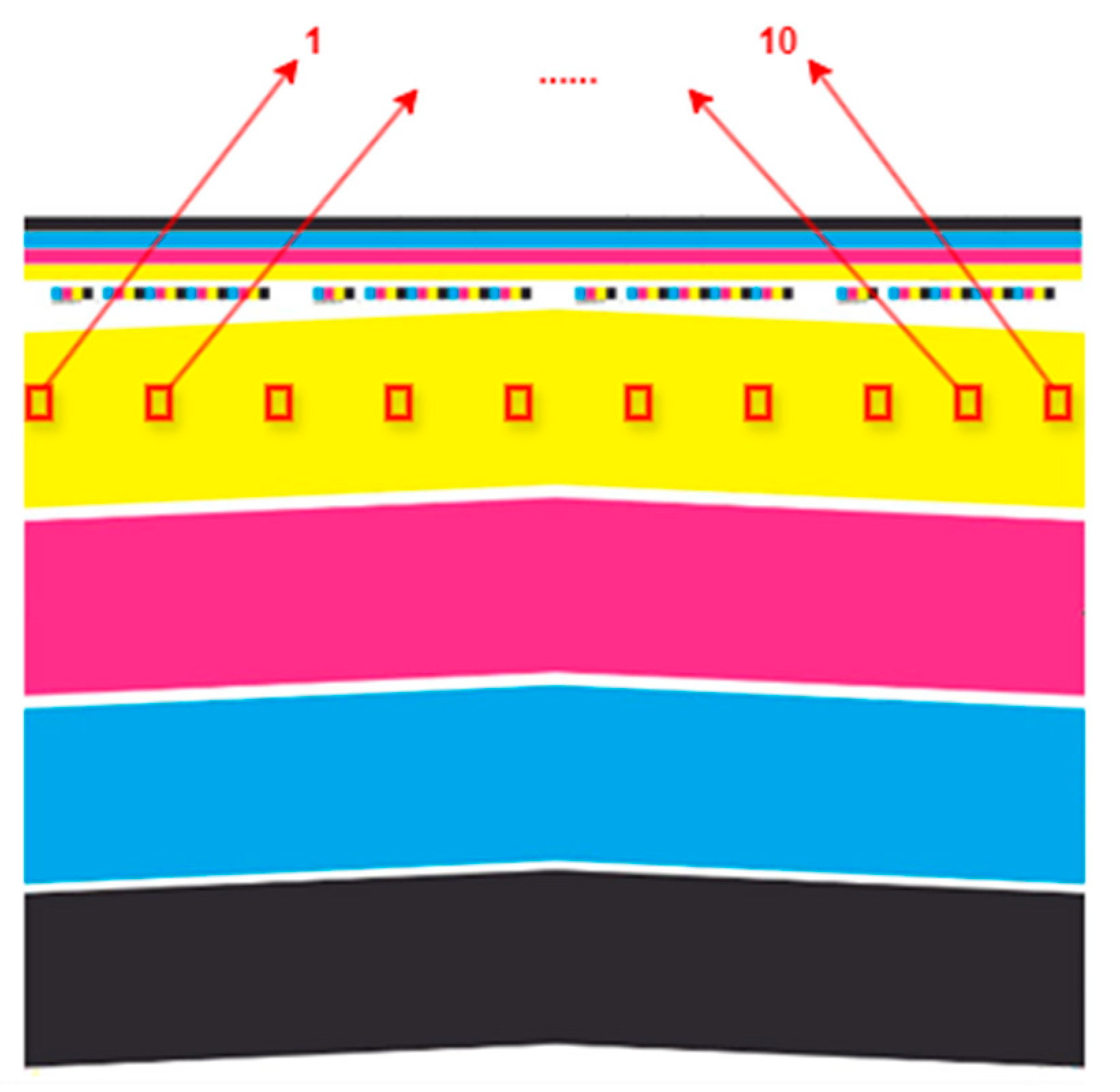
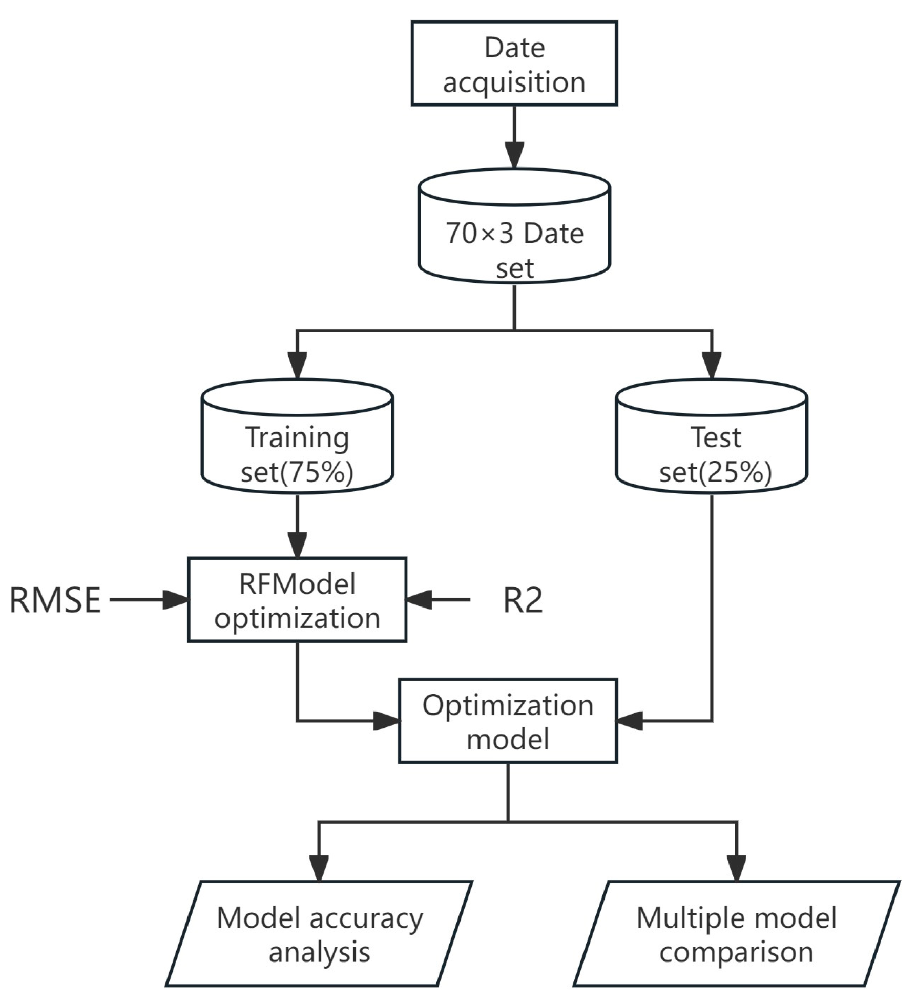
3.2. Data Acquisition

In offset printing (lithography) process control, the clarity of measurement conditions is essential to ensure both color consistency and process compliance. In this experiment, the ambient temperature was maintained at 23 °C, and the relative humidity was set to 60%. The four-color printing sequence was set to black, cyan, magenta, and yellow. The screen ruling was 72 lines/cm, the printing speed was set at 5000 sheets/hour, and the printing pressure was adjusted to 200–300 N using a printability tester.

The experimental samples employed an ink balance chart from the G7 color management process, a widely used tool in industrial production. Figure 3 shows a schematic diagram of the sample sheet. Samples were collected every 10 sheets starting from the beginning of printing to monitor the ink balance process. The test samples were allowed to rest for more than 48 h to ensure complete ink drying. A spectrophotometer was used to select 10 evenly distributed measurement points on the printed sheet, recording the L*, a*, and b* colorimetric values, as well as the density values. The spectrophotometer used diffused illumination with an 8° receiving geometry, and the M1 measurement mode was activated to enable metameric correction. The densitometer filter setting was selected as Status T. The D65 standard light source, which simulates average daylight conditions, was employed to ensure consistent color evaluations across different samples. Additionally, a 2° standard observation angle was used to comply with industry standards for visual color perception. The reference point was selected as the actual paper white rather than absolute white to better align with human visual perception.

To minimize the influence of external factors on measurement accuracy, the tests were conducted in a controlled environment with stable temperature and humidity, thus preventing ink color variations caused by uneven drying. These stringent experimental procedures ensured that the collected data accurately reflected the ink balancing process, thereby providing reliable results for further analysis.

The data were randomly divided into a training set (75%) and a test set (25%) using the scikit-learn library in Python 3.11.5. The training set was used to construct RF models, while the test set was used for model validation and evaluation. To ensure the reproducibility of the dataset division and maintain data balance, the randomness of the data split was controlled by pairing the stratified_regression with the stratify parameter in the code.

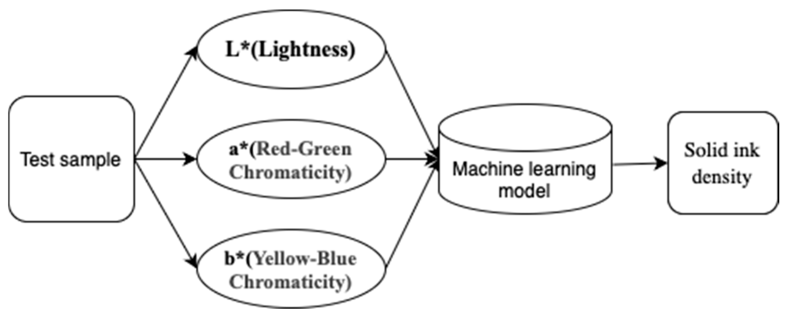
3.3. Optimal Solid Ink Density Matching Model

In the offset printing process, increasing the ink output from the ink rollers leads to an increase in substrate ink thickness and ink density, resulting in higher color saturation and more vivid colors in the printed material [19] However, as the Lamb-Bill equation demonstrates, once a certain value is reached, further increases in ink thickness no longer occur. Continuing to increase the ink amount may cause disproportionate dot expansion, resulting in gradation issues and other problems in the printed image. Therefore, during the pre-press color correction stage, it is crucial to find a method to determine the optimal solid ink density, ensuring that the density adjustment leads to the best possible print quality.

Traditional solid ink density determination in printed materials primarily relies on the printing parameters of relative contrast (K value), typically calculating the optimal solid ink density based on the density difference ratio at 75% or 80%. This method lacks control over the visual perception of printed materials and is being gradually phased out by printing companies. Relying solely on density control is insufficient to ensure consistent color quality. Integrating chromaticity control helps mitigate color deviations caused by variations in the printing environment, paper types, ink concentrations, and other influencing factors. Moreover, chromaticity control enables precise adjustments across different paper and ink types, ensuring uniform color quality across multiple print batches. This paper aims to utilize the international standard ISO 12647-2:2013, which specifies the colorimetric value requirements for printing solid ink color blocks, to control the optimal solid ink density. In printing, solid ink color blocks refer to areas of printed material where a single, uniform ink coverage is applied without the use of halftone screens or gradients. These blocks represent 100% ink density and are used in color management and quality control to assess color accuracy and consistency in the printing process.

To investigate the relationship between ink density and chromaticity coordinates, the Pearson correlation coefficient is calculated to quantify the degree of association between the variables. The Pearson correlation coefficient is a statistical measure that quantifies the strength and direction of a linear relationship between two variables. A key property of this coefficient is that it remains unaffected by changes in the position or scale of the variables. This property allows it to be effectively applied in analyzing the relationship between abstract chromaticity parameters and controllable ink density values. Let the L, a, and b chromaticity coordinate values be denoted as X = {$x_1$, $x_2$, …, $x_i$}, and the corresponding solid ink density values as Y = {$y_1$, $y_2$, …, $y_i$}. The Pearson correlation coefficient is defined as shown in Equation (11).

$$r={\displaystyle \frac{{\displaystyle \sum (x_i-\overline{x})}(y_i-\overline{y})}{\sqrt{\left({\displaystyle \sum {(x_i-\overline{x})}^2}\right)\left({\displaystyle \sum {(y_i-\overline{y})}^2}\right)}}}$$

(11)

The Pearson correlation coefficient r, as defined by the equation, ranges between −1 and 1. The closer the r value is to either extreme, the stronger the linear relationship between the two variables. When the correlation between the variables is weak, the r value approaches zero. In general, an absolute value of r greater than zero (∣r∣ > 0|) is considered indicative of a linear relationship between the variables.

The Pearson correlation coefficients were computed by substituting the four data sets—L, a, b, and Ds—into Equation (11), as shown in

Table 3. Pearson correlation coefficients of different ink colors.

Ink	L	a	b
C	0.92	−0.82	0.78
M	0.89	−0.79	0.82
Y	0.88	−0.86	0.85

.

The results show that the Pearson coefficients for the L values exceed 0.8, while those for the a and b values are approximately 0.8. Although the L, a, and b chromaticity coordinates exhibit strong linear relationships with solid ink density, the correlations are not perfectly positive. This suggests that in practical production settings, ink density cannot be reliably adjusted based solely on visual judgment or intuition. Furthermore, comparison of the Pearson coefficients indicates that the strength of correlation between chromaticity coordinates and solid ink density varies among the components. This suggests that even when ink density increases uniformly, the changes in chromaticity coordinates across different directions are not proportionally linear.

Based on this analysis, the present study moves beyond traditional approaches to determining optimal solid ink density. Instead, it introduces a nonlinear modeling approach to quantify the relationship between chromaticity and density, with the goal of identifying optimal solid ink density parameters for pre-press calibration and process control.

A review of the existing literature indicates a nonlinear relationship between the colorimetric value of the print color block and its density value. To establish the relationship between colorimetric values and density values, in this paper, we model the relationship between the input (colorimetric value of the print color block) and the output (solid density of ink) using a Random Forest machine-learning model. Specifically, the sample data of solid ink color block density values and colorimetric values from multiple print proof are used to construct a matching model with multiple inputs and a single output. Figure 4 shows the structure of the model. Initially, cyan, magenta, and yellow inks were printed at 100% dot coverage on coated paper. The solid ink density of each color was then measured, and the corresponding CIELAB color coordinates were recorded. Seventy data sets were collected for each ink color. The dataset is subsequently divided into a training set (75%) and a testing set (25%). The model’s hyperparameters are optimized using correlation coefficients and mean square error, and the optimized model is then evaluated for performance. To further justify the choice of the Random Forest method, the final step involves comparing the performance of the Random Forest model with that of other machine-learning models to ensure the selection of the most optimal model.

3.4. Data Pre-Processing

Data must be pre-processed before being used to build a predictive model to ensure its accuracy. Data normalization is a commonly used pre-processing technique in machine learning [26]. Since the dataset in this paper contains features with varying ranges, the training process is accelerated and made more efficient by eliminating scale differences between the features. All data were normalized using the mapping function (Equation (12)) to fit within the range from 0 to 1. Here, $x_{\max }$ and $x_{\min }$ represent the maximum and minimum values of the input variables before normalization, while $x_{\mathrm{scale}}$ and $x$ denote the data values before and after normalization, respectively.

$$x_{\mathrm{scale} }={\displaystyle \frac{x-x_{\min }}{x_{\max }-x_{\min }}}$$

(12)

The dataset was processed using the aforementioned standardization method based on the selected samples to obtain a dataset suitable for the Random Forest model. As an example, the processed C-color L*a*b* and solid ink density values (D) are shown in

Table 4. Hyperparameters in the Random Forest algorithm.

Name	Default Value	Description
n_estimators	100	The number of decision trees to control the complexity and stability of the model.
max_depth	None	The maximum depth of the tree. If the value is “none” the node will continue unless all leaves are pure.
min_samples_split	2	The minimum number of samples required to divide nodes.
max_leaf_num	None	Maximum number of leaf nodes.

.

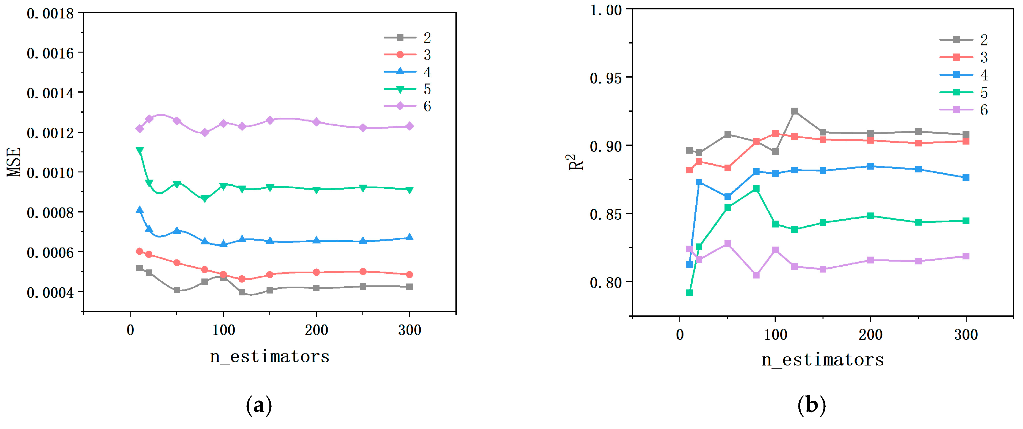
3.5. Hyperparameter Optimization in Random Forest Algorithms

The performance of the model critically depends on the selection of hyperparameters, which must be thoroughly discussed and determined prior to constructing a Random Forest model. Table 4 presents the hyperparameters commonly required for configuring the Random Forest model. Key hyperparameters include the minimum number of samples required to split a node, the number of decision trees, the maximum depth of trees, the maximum number of features considered for splitting, and the maximum number of leaf nodes [27,28,29]. These parameters are typically determined empirically, and their relative importance varies depending on the dataset employed. For most datasets, only a limited subset of hyperparameters significantly influences model outcomes. Notably, the number of decision trees and the maximum tree depth exhibit the highest prioritization, followed by the minimum samples required for node splitting and the maximum leaf node constraints. Due to the limited sample size in this study and the fact that the maximum tree depth constrains the impact of the minimum leaf node count on the forest, the maximum depth and maximum node count were set to their default values. Instead, optimization focused on the minimum number of samples required for node splitting and the number of decision trees, as these have a greater influence on the model’s performance. Since the interaction between the two hyperparameters is minimal, each hyperparameter can be optimized independently.

(1) Determine the number of decision trees

The Random Forest model’s size is determined by the quantity of decision trees. According to earlier research, the Random Forest prediction model’s capacity for generalization steadily stabilizes as the number of decision trees rises. An overabundance of decision trees, however, may slow down the model’s pace of convergence and reduce its applicability in real-world scenarios. For this reason, choosing the right number of decision trees is essential when building a model.

Since the sample size in this study is small, the number of decision trees was set within the range from 0 to 300 during the construction of the model. The ideal parameters are chosen by comparing the mean squared error (MSE) values for various numbers of decision trees after the corresponding MSE values for the three colors are determined independently. Figure 5 displays the MSE values for varying numbers of decision trees. The vertical axis shows the MSE values, and the horizontal axis shows the number of decision trees. Based on the training results of the three ink datasets, the MSE reached its minimum when the number of decision trees was set to 100 for cyan ink, 50 for magenta ink, and 100 for yellow ink. Currently, the model performance is the best. Therefore, it can be concluded that the model’s output is optimal when the number of decision trees is set to the above-mentioned values.

(2) Determine the minimum number of nodes

The “min_samples_split” parameter in decision trees defines the minimum number of samples required to divide an internal node. Specifically, if a node contains fewer samples than the defined threshold, it remains a leaf node and is not further divided. Adjusting the “min_samples_split” parameter regulates tree growth, preventing excessive complexity, mitigating overfitting, and enhancing training efficiency. As stated in the scikit-learn documentation, the default value for this parameter is two. In this study, the minimum number of samples required to split a node was selected from the empirically recommended range of two to six. Subsequently, MSE and R² were calculated for the model using different numbers of decision trees, with the minimum sample size varied between two and six. Given that all three color sample groups had identical sample sizes, the C-color sample dataset was utilized for analysis. As illustrated in Figure 6, setting the minimum leaf node count to two results in the lowest MSE and highest R², indicating optimal model performance. Consequently, two was determined to be the optimal minimum leaf node value for this study.

3.6. Other Machine-Learning Methods for Comparison

To emphasize the predictive accuracy of the proposed model in determining the optimal solid ink density for printing materials, machine-learning algorithms recognized for their robustness with small sample sizes and low-dimensional datasets were selected for comparative validation, based on the specific characteristics of the dataset used in this study. The selected models included Gradient Boosting (GB), Artificial Neural Network (ANN), Support Vector Regression (SVR), and Polynomial Regression, all trained on the same dataset. Among these, Gradient Boosting (GB) is a robust machine-learning method widely used for regression and classification tasks [30]. It constructs an ensemble predictive model by iteratively adding new learning nodes and enhances prediction accuracy through tunable parameters and various loss functions. Benefiting from its strong nonlinear modeling capability, Gradient Boosting demonstrates excellent generalization performance across different types of datasets, including high-dimensional datasets with numerous features and small datasets. Artificial Neural Networks (ANN) are computational models inspired by biological neural systems, with a core structure comprising synapses, an adder, and an activation function [31]. The connection strength is represented by weights, where positive weights indicate excitatory connections and negative weights indicate inhibitory connections. The adder computes the weighted sum of input signals, while the activation function enables the model to approximate complex functions, generalize patterns, and effectively learn through parameter adjustments. ANN is capable of modeling highly complex nonlinear relationships and is frequently applied in deep learning tasks, particularly excelling in processing large-scale and high-dimensional data. In this experiment, a Multilayer Perceptron (MLP)—a classical feedforward artificial neural network model—was employed for data processing. Polynomial Regression (PR) is an extension of linear regression, commonly used to model nonlinear relationships between dependent and independent variables [32]. By incorporating polynomial terms of independent variables into the model, PR effectively captures nonlinear patterns in data. This model is particularly suitable for applications with small sample datasets, offering low computational cost and requiring minimal computational resources. Support Vector Regression (SVR) is a regression model based on Support Vector Machines (SVM) that constructs a hyperplane in a high-dimensional space to fit the data while minimizing model complexity [33]. SVR is particularly well-suited for applications requiring precise data predictions while preventing overfitting. However, due to its high computational complexity, it is not ideal for large-scale datasets and is highly sensitive to hyperparameter selection.

For all machine-learning methods, input parameters were standardized to L*, a*, and b* stimulus values, with model outputs set to solid ink density values. Identical training and validation datasets were used across all tested machine-learning methods. The hyperparameters of the models were optimized using the ten-fold cross-validation method [34]. This method divides the dataset into ten equal subsets, with nine subsets used for training and one for testing in each iteration. The optimized parameter values are presented in the

Table 5. Model hyperparameters after optimization of different models.

Model	Best Params
Random Forest	Max features: none min samples leaf: 1 min samples split: 2
SVR	c: 0.1 gamma: 0.1
Polynomial Regression	Linearregression fit intercept: false Polynomial features degree: 2
ANN	activation: tanh alpha: 0.01 hidden layer sizes: 100 solver: adam
GB	Learning rate: 0.2 Max depth: 5 Min samples leaf: 1 Min samples split: 5 n_estimators: 200

.

3.7. Evaluation Indicators

For the Random Forest prediction model, four evaluation metrics are selected to assess its performance: the coefficient of determination (R²), mean absolute error (MAE), mean squared error (MSE), and root mean squared error (RMSE). R² represents the goodness-of-fit between variables; the closer the value is to 1, the better the fit. RMSE represents the deviation between predicted and actual values. The evaluation metrics, including MSE, are expressed in Equation (13). The expressions are shown in Equation (13).

$$\begin{gathered} \begin{array}{c}{R}^2=1-{\displaystyle \frac{{\displaystyle \sum _{i=1}^N{\left(y_i^{\mathrm{mea} }-y_i^{\mathrm{pre} }\right)}^2}}{{\displaystyle \sum _{i=1}^N{\left(y_i^{\mathrm{mea} }-E\left[y^{\mathrm{mean} }\right]\right)}^2}}}\\ MSE={\displaystyle \frac{1}{N}}{\displaystyle \sum _{i=1}^N{\left(y_i^{\mathrm{mea} }-y_i^{\mathrm{pre} }\right)}^2}\\ RMSE=\sqrt{{\displaystyle \frac{1}{N}}{\displaystyle \sum _{i=1}^N{\left(y_i^{\mathrm{mea} }-y_i^{\mathrm{pre} }\right)}^2}}\end{array} \\ \mathrm{MAE}={\displaystyle \frac{1}{n}}{\displaystyle \sum _{i=1}^n\left|y_i-{\widehat{y}}_i\right|} \end{gathered}$$

(13)

where $y_i^{\mathrm{mea}}$ is the measurement; $y_i^{\mathrm{pre}}$ is the predicted result; E[$y_i^{\mathrm{mea}}$] is the mean of $y$; N is the number of samples; and k is the number of independent variables.

4. Results

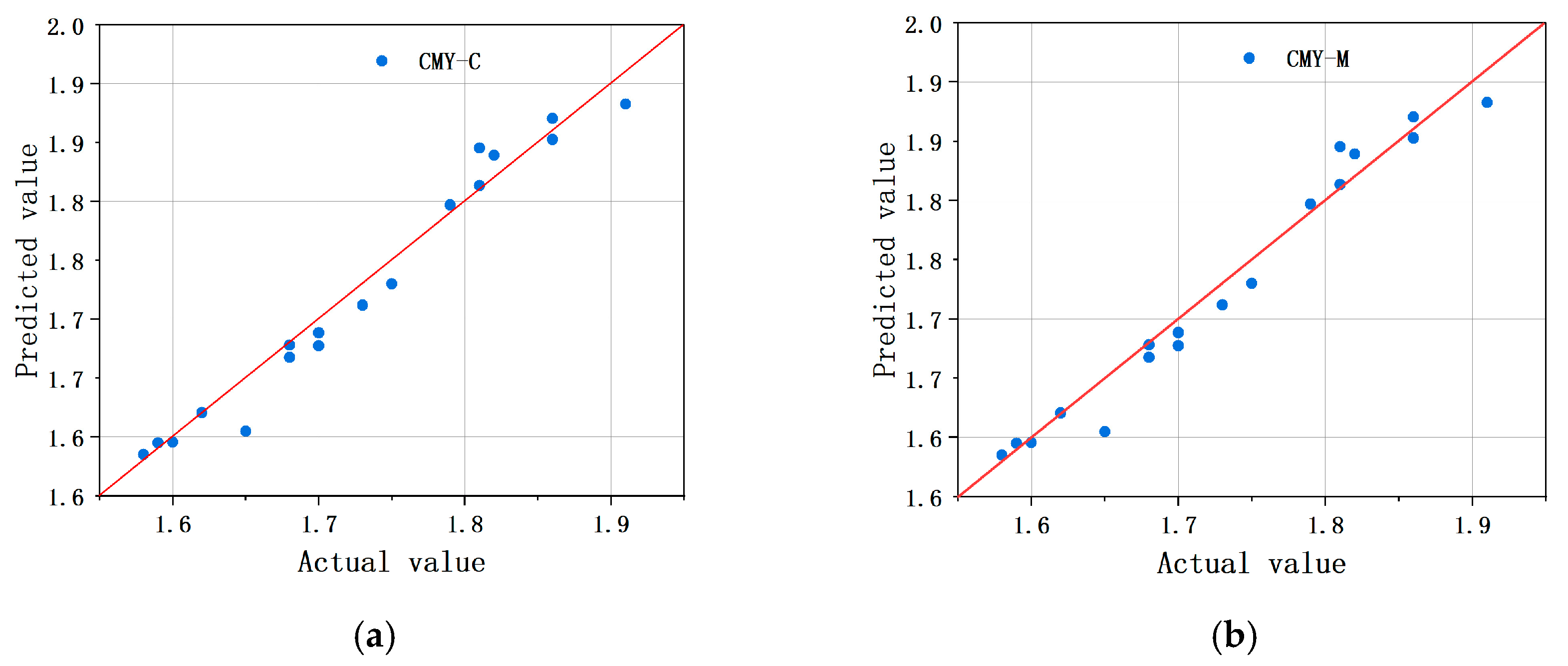
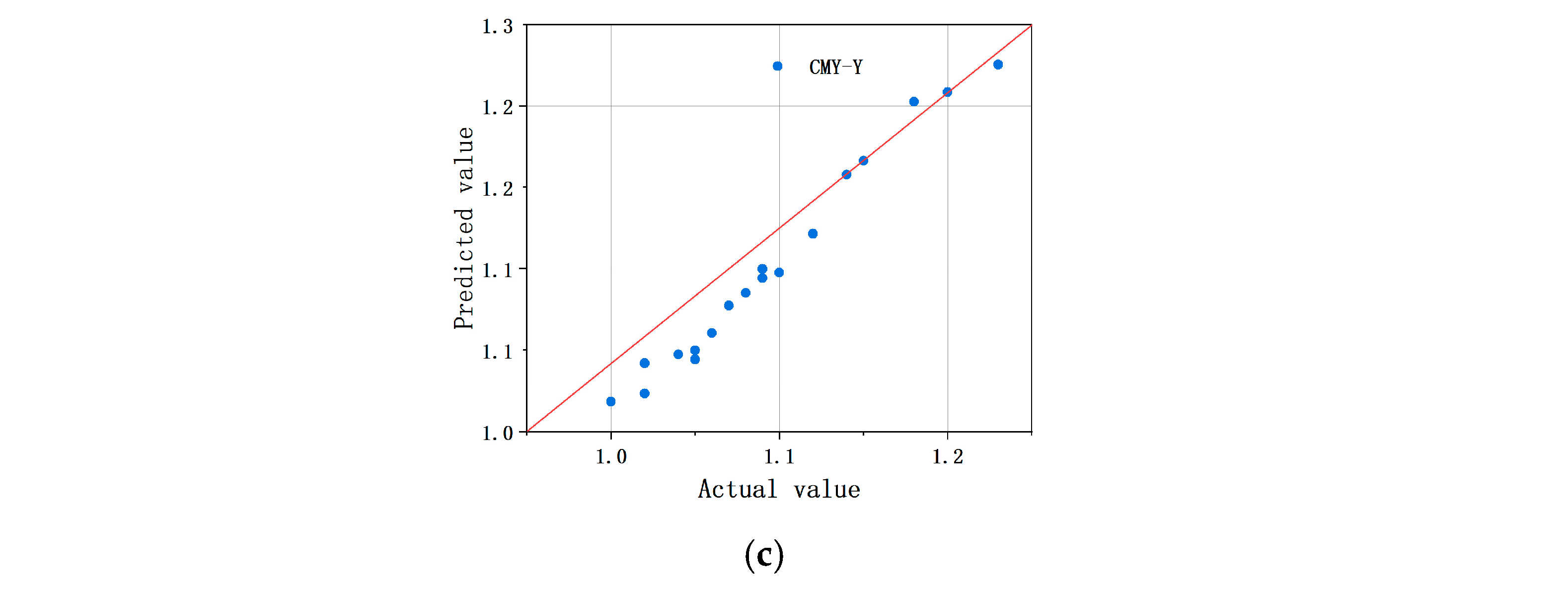
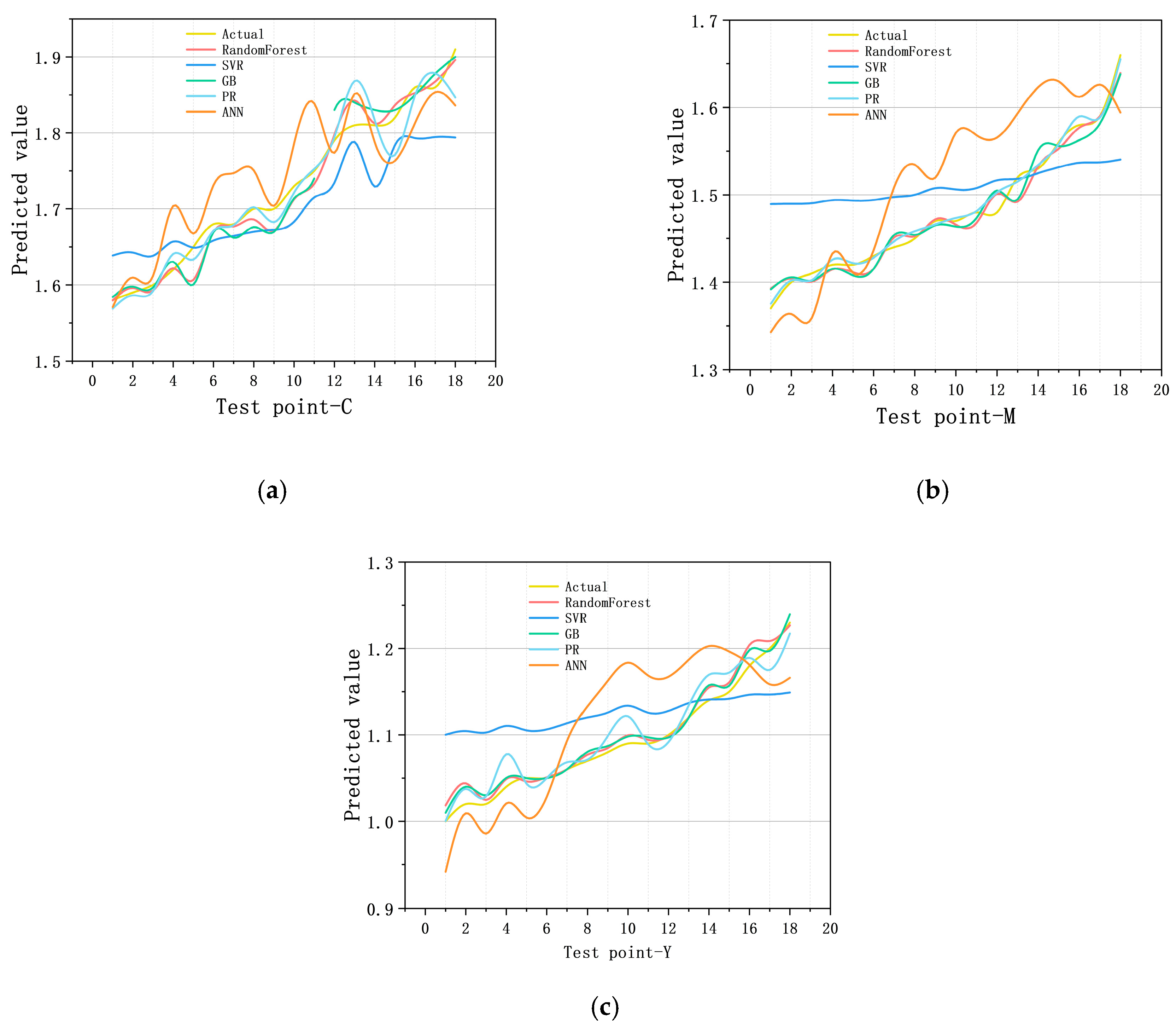
4.1. Model Training Results

The trained model can predict the optimal solid ink density for printed materials. Since these target values are discrete, the task can be considered a regression problem. MAE, MSE, RMSE, and R² were used as evaluation metrics to assess the model’s accuracy. The model parameters were set to the optimized values discussed earlier in the paper and validated.

After training the model with sample data, the predicted values were compared to the actual data. Figure 7 shows the measured solid ink density values for three different inks (C, M, and Y), compared with the predicted values. As shown in the Figure, the training results of the Random Forest prediction model align well with the actual test results. The prediction model generated by the algorithm after training on a large number of samples, more accurately predicts the solid ink density values for different colors of samples. This verifies that the model has strong generalization ability.

To further validate the model’s training results, the three-color solid ink color block CIELAB L*a*b* values required by the company providing the experimental data were used as input. The model’s output density values were recorded, and the optimal solid ink density values determined here were compared to the Chinese national standard GB/T 17934.1-1999 [35]. Additionally, the range of solid ink densities calculated from the validation set was compared with the Chinese national standard GB/T 17934.1-1999. The model’s accuracy was assessed based on the degree of approximation of these values, which are presented in

Table 6. Standard colorimetric values.

Printing Ink	L*	a*	b*
C	56	−35	−44
M	45	68	−3
Y	83	−5	87

and

Table 7. Comparison of calculated solid ink densities with standard density values.

Printing Ink	Calculated Density Range	Optimum Solid Ink Density	China’s National Standard Range
C	1.57–1.92	1.62	1.5–2.0
M	1.56–1.91	1.61	1.3–1.6
Y	1.02–1.22	1.08	0.9–1.1

.

The verification results show that the optimal solid ink density values for the three ink colors output by the model fall within the range specified by the GB/T 17934.1-1999 standard. Specifically, the optimal solid ink density for cyan (C) and yellow (Y) inks are within the standard ranges of 1.5 to 2.0 and 0.9 to 1.6, respectively. The optimal solid ink density for magenta (M) ink is 1.61, which aligns with the standard range of 1.3 to 1.6. Furthermore, the calculated density for cyan ink complies with the range set by the Chinese national standards. However, the upper limits of the calculated density ranges for magenta and yellow inks are 1.91 and 1.22, respectively, exceeding the standard values by 0.31 and 0.12.

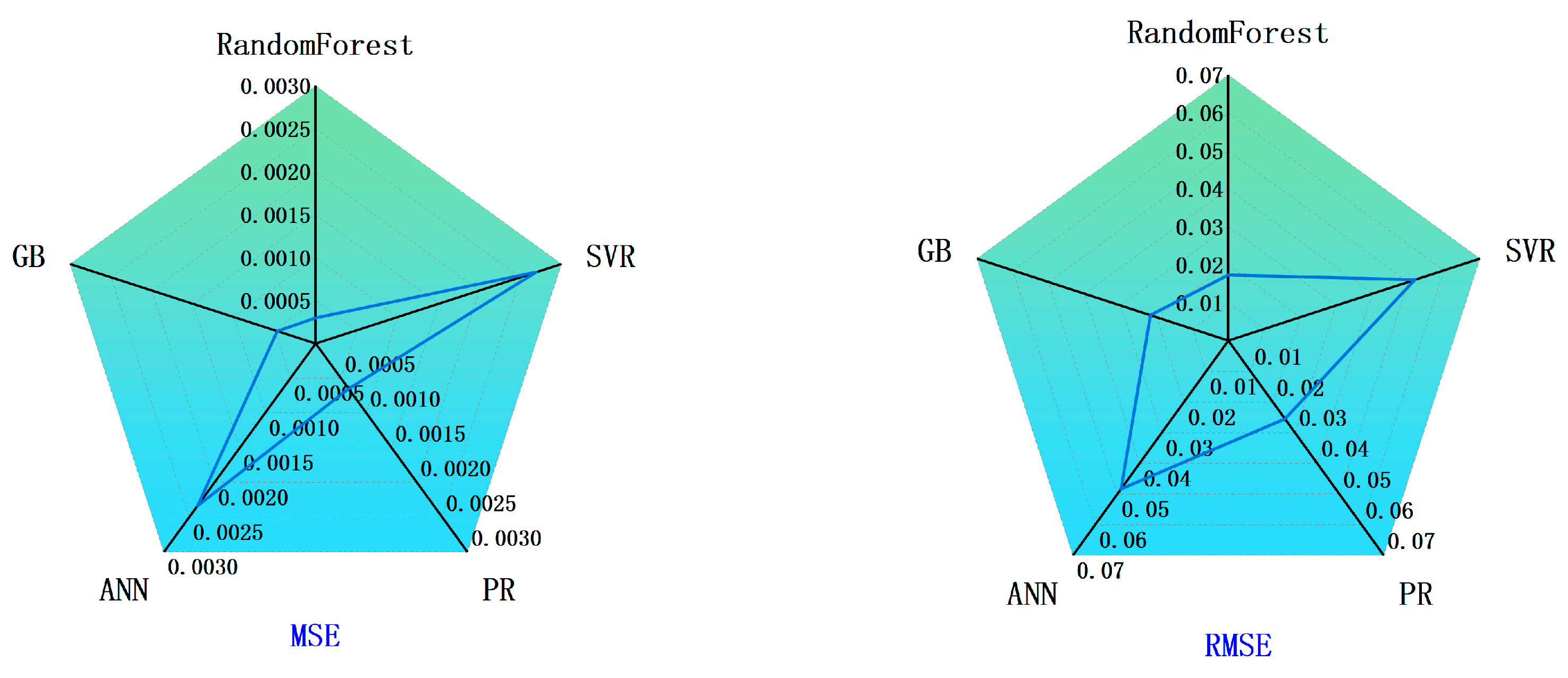
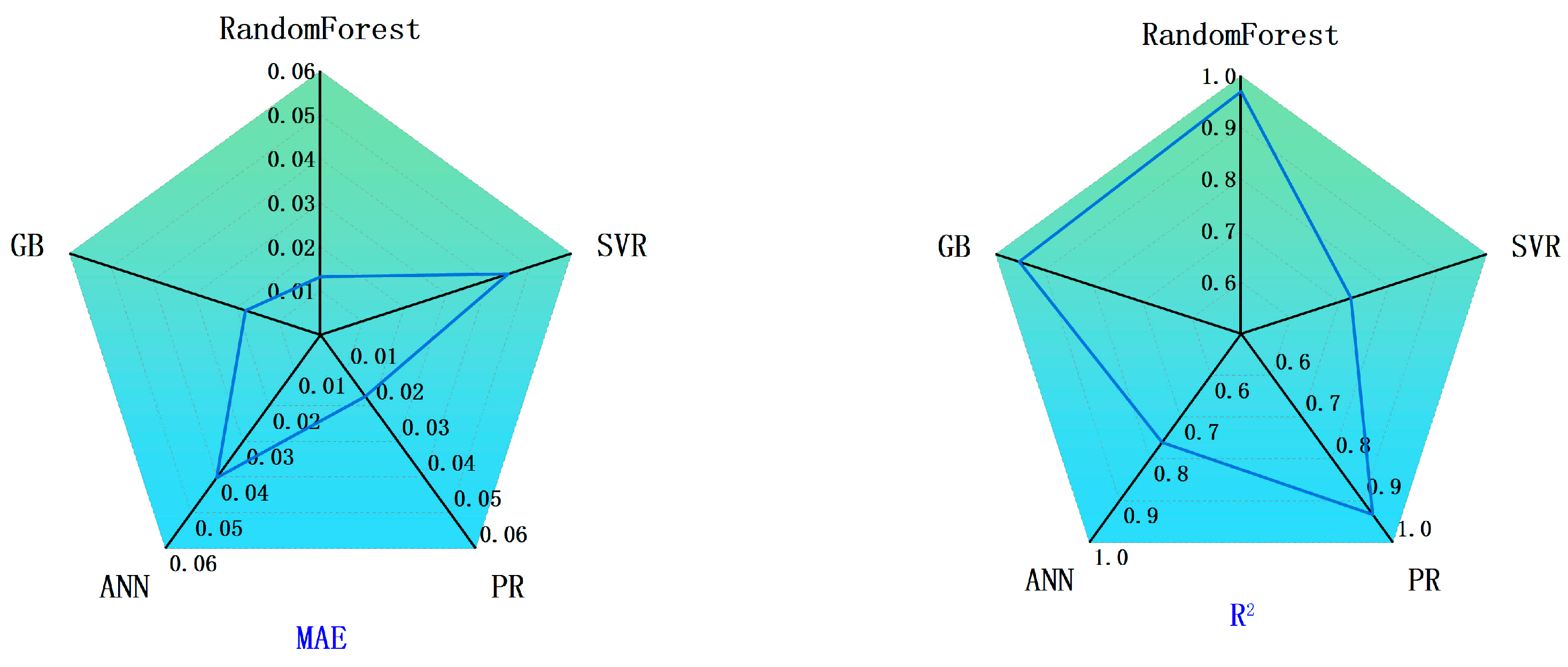
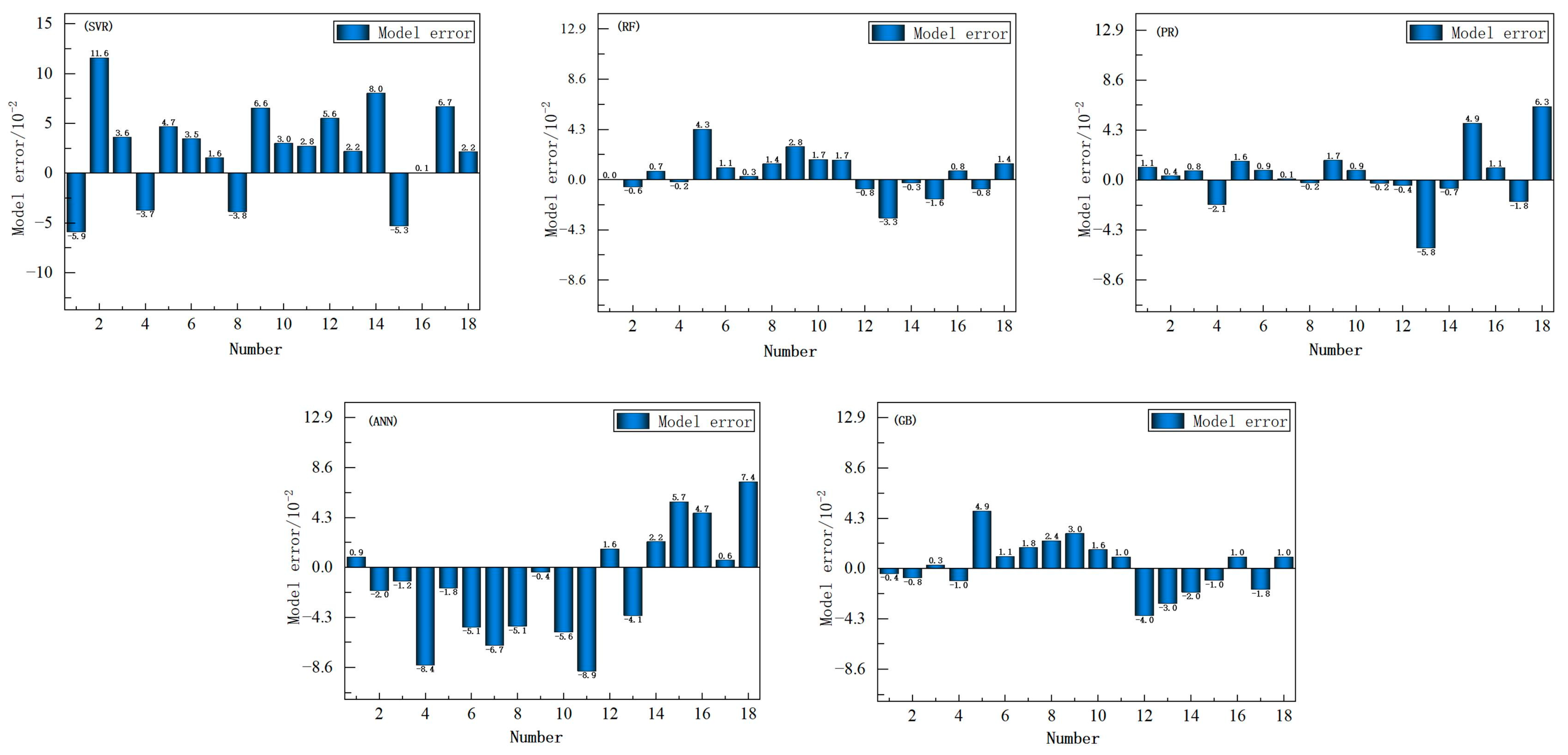
4.2. Comparative Evaluation of Model Performance

In this study, MAE, MSE, and RMSE were employed to evaluate model accuracy, where smaller values indicate higher prediction accuracy. The R² metric was used to assess model fit, with larger values signifying better fit.

Table 8. Model metrics after different model training.

Model	MSE	RMSE	R2	MAE
Random Forest	0.00029	0.0173	0.9692	0.0131
SVR	0.00269	0.0518	0.7233	0.0448
Polynomial Regression	0.00065	0.0255	0.9332	0.0173
ANN	0.0023	0.0483	0.7605	0.0401
GB	0.00046	0.0216	0.9513	0.0178

and Figure 8 present performance comparison data for solid ink density prediction in prints. These results indicate that all machine-learning models demonstrate strong predictive capabilities. The four accuracy metrics (R², MSE, RMSE, and MAE) for both training and test sets reveal that the Random Forest model outperforms traditional prediction models for the colorimetric value and density dataset collected in this experiment. The Random Forest model demonstrated superior performance over the comparative models across all key evaluation metrics. Specifically, when compared to the high-performing polynomial regression model, it achieved reductions of 0.00036 in MSE, 0.0082 in RMSE, and 0.0042 in MAE. Relative to the gradient boosting model, the reductions in MSE, RMSE, and MAE were 0.00017, 0.0043, and 0.0047, respectively. These consistently lower error values—particularly the 7.8% to 11.2% reduction in MAE—suggest that the Random Forest model offers improved consistency between predicted and actual measured values. The Gradient Boosting (GB) model also demonstrates strong regression performance. It has an R² value only 0.018 lower than the Random Forest model, an MSE of 0.00046, an MAE of 0.0178, and an RMSE of 0.0216. The Polynomial regression model also performs well, with an MSE of 0.00065, an RMSE of 0.0255, an MAE of 0.0173, and an R² of 0.0933. However, its capacity to handle solid ink density is somewhat limited compared to the previous two models.

In contrast, the ANN and SVR models exhibit significantly lower accuracy, with R² values of 0.7605 and 0.7233, respectively. Their error metrics are notably higher than those of the other models. Conversely, the accuracy of the Random Forest model is superior to that of both ANN and SVR models. Its R² value is 0.246 higher than the SVR model and 0.036 higher than the polynomial regression model, indicating superior fit.

The effectiveness of the machine-learning models in solid ink density prediction is illustrated in Figure 9. A closer alignment of the predicted value curve with the target true value curve indicates better predictive performance. Among the models, Random Forest, Polynomial Regression, and Gradient Boosting exhibit a closer fit to the true value curve, with smaller deviation values, demonstrating higher accuracy and precision.

To improve the accuracy of quantitative evaluation, the discrepancies between the predicted and actual values for each ink color in the validation set were visualized. Figure 10 presents the error statistics of the optimal solid ink density prediction model for cyan ink. As illustrated in the figure, the SVR model exhibited the widest prediction error range, with a maximum error of 1.16 × 10⁻¹ and a minimum error of 1 × 10⁻³. Similarly, the ANN model yielded a maximum prediction error of 8.9 × 10⁻² and a minimum of 4 × 10⁻³. The PR and GB models demonstrated improved accuracy over SVR and ANN, with maximum errors of 6.3 × 10⁻² and 4.9 × 10⁻², respectively. The RF model showed the smallest prediction error range, with a maximum error of 4.3 × 10⁻² and a minimum of 0.

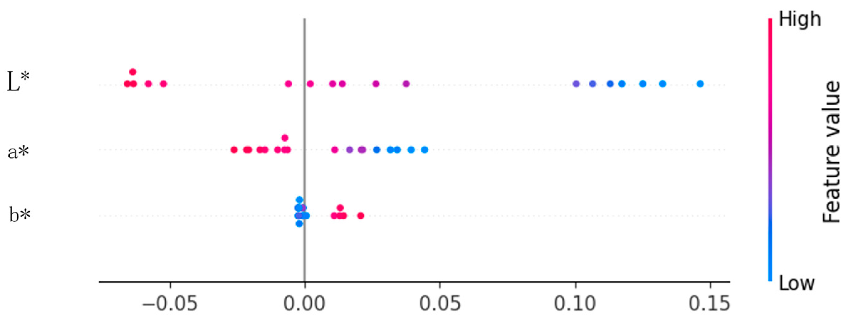
4.3. Feature Importance Analysis

The SHAP (SHapley Additive exPlanations) method was used to quantify the contributions of the three chromaticity features to the predicted solid ink density. Based on the computed SHAP values, the input features were analyzed and ranked according to their average influence.

Table 9. The name and SHAP value of the model feature variable.

Feature Name	SHAP Value
L*	0.0345
a*	0.0069
b*	0.0083

displays the mean SHAP values corresponding to each feature. A SHAP beeswarm plot was generated to visualize the influence of the three features within the Random Forest model. The bee swarm plot is shown in the Figure 11. In this plot, the color of each data point reflects the magnitude of its corresponding feature value. Data points located to the right of the vertical axis (positive SHAP values) indicate features that contribute positively to the prediction, whereas those on the left (negative SHAP values) suggest a suppressive effect. The analysis revealed that the L* value (lightness) exerted the strongest influence on the prediction of solid ink density, with a mean SHAP value of 0.0345.

4.4. Neutral Gray Chromaticity Evaluation

To assess the applicability of the optimal solid ink density values produced by the model, the printing process was conducted using the target values calculated in Table 8. Sample sheets were then printed, and gray balance performance was evaluated by measuring the L, a, and b values in the CIE Lab color space for gray patches composed of three CMY combinations: 25C19M19Y, 50C40M40Y, and 75C66M66Y. This evaluation aimed to analyze color shift tendencies across varying tonal levels of the gray scale.

Six qualified sample sheets were selected, and the average neutral gray colorimetric values of the gray patches were computed. The results are presented in

Table 10. Neutral gray colorimetric values of gray patches composed of CMY combinations.

Index	25C19M19Y			50C40M40Y			75C66M66Y
	L	a	b	L	a	b	L	a	b
1	76.1	0.1	−0.3	58.4	−0.5	−0.7	37.6	−1.5	−0.7
2	75.9	0.3	−0.5	57.5	0.8	0.3	36.5	−1.8	−1.3
3	75.3	0.5	−0.6	57.7	−0.3	−0.2	35.7	−1.3	−1.2
4	75.7	0.4	−0.2	58.8	0.9	0.8	36.8	−0.9	0.8
5	76.1	0.3	−0.4	57.9	0.8	−0.5	37.9	−1.8	−0.5
6	75.3	0.2	−0.3	59.4	0.6	−0.4	38.4	−1.6	−1.4
Average	75.7	0.3	−0.3	58.2	0.3	−0.1	37.1	−0.1	−0.7

. As shown in Table 5, the samples produced under process control using the model-derived optimal solid ink density values demonstrated satisfactory gray balance performance. The average deviations in the a and b channels for all three overprint combinations were below one.

5. Discussion

The validation results demonstrate that the machine-learning model proposed in this study effectively establishes a quantitative relationship between chromaticity coordinates and ink density values, thereby aiding manufacturers in identifying the optimal solid ink density parameters prior to production. Among all the machine-learning models evaluated, the Random Forest (RF) model achieved superior performance in terms of both accuracy and reliability. Additionally, visual analysis confirmed that the RF model did not exhibit signs of overfitting. These findings underscore the importance of selecting a high-performance model during the calibration stage of the printing process to ensure accurate prediction of optimal solid ink density.

During validation with the standard solid ink colorimetric values, slight deviations were observed in the case of magenta ink. However, further analysis indicated that these deviations resulted from differences between the paper and ink used in this study and those prescribed by the Chinese national standards. Paper brightness, smoothness, ink absorption, and viscosity significantly affect color intensity under identical ink density conditions. Experimental measurements indicate that the ink viscosity in this study was 19 Pa·s, whereas the Chinese Light Industry Standard GB/T 2624-2012 [36] (“Sheet-Fed Offset Printing Ink”) specifies a recommended viscosity range of 10–15 Pa·s. Excessive ink viscosity compromises fluidity, resulting in higher solid density and uneven ink distribution.

All regression models successfully achieved density matching. Although Artificial Neural Networks (ANN) and Support Vector Regression (SVR) are popular regression methods and have demonstrated strong performance on many datasets, their regression accuracy on the Lab* colorimetric values dataset was lower than that of polynomial regression and random forest. Experimental results indicate that the regression coefficients for ANN and SVR were only 0.723 and 0.76, respectively, which are suboptimal for practical applications. Due to ANN’s high sensitivity to data, it exhibited significant bias in both low- and high-density regions [37]. This sensitivity hinders its ability to handle discrete datasets, particularly when the number of data points is limited, thereby reducing prediction accuracy. Additionally, the stochastic nature of small datasets makes ANN training more susceptible to the influence of initial weights, often leading the model to converge to different local optima and resulting in unstable training. While SVR is effective in capturing nonlinear relationships in certain applications, it exhibited higher error values and weaker predictive performance in the dataset used in this study compared to other machine-learning models. SVR relies on well-tuned hyperparameters to achieve optimal generalization. However, in limited datasets, hyperparameter tuning becomes challenging, increasing the risk of underfitting. Furthermore, SVR struggles to accurately estimate an appropriate kernel mapping when data is scarce, leading to reduced generalization capability. Improving model performance may require further adjustment of model parameters. In the feature importance analysis, the SHAP values derived from the Random Forest model reveal that the L* value has the highest mean SHAP score, indicating that lightness exerts the greatest influence on the model’s predictive output and represents the most critical feature. This finding also indicates that increases in solid ink density lead to more pronounced changes in the lightness of the printed ink on the paper.

Furthermore, the results obtained from implementing the model-generated optimal solid ink density values for process control and sample sheet printing indicate that density regulation can effectively assist practitioners in maintaining gray balance, as evidenced by the neutral gray chromaticity parameters. In the absence of press-specific requirements, the solid ink color patches on printed samples are generally expected to comply with the international standard ISO 12647-2:2013. However, in practical applications, the target colorimetric values are not strictly constrained by these standards and may be adjusted to accommodate specific production requirements.

It is important to emphasize that this study is the first to apply the Random Forest algorithm to the prediction of solid ink density in offset printing. Compared with other machine-learning algorithms, the Random Forest method exhibits greater robustness against overfitting, especially when trained on small-scale datasets. The modeling approach proposed in this study is applicable not only to the offset printing conditions used in the experiments but also exhibits strong portability and scalability. Unlike traditional physical modeling approaches, the quantitative relationship between colorimetric values and ink density established through Random Forest is independent of equipment or substrate characteristics and is based entirely on measured data. As a result, practitioners are not required to account for how specific presses or materials affect ink color reproduction. With appropriate modifications to the input features, the proposed method can be extended to various paper and ink combinations, as well as to spot color printing scenarios. Furthermore, the model offers both data support and algorithmic foundations for the development of intelligent color control systems in printing environments, facilitating the transition from traditional printing workflows to a “predictive control—closed-loop optimization” paradigm. Therefore, the proposed approach holds significant promise for both industrial application and academic research.

6. Conclusions

This study focuses on the first-time application of the Random Forest algorithm in modeling offset printing color control systems. The objective is to determine the optimal solid ink density of test samples during the pre-press stage of printing production, highlighting the method’s strong practical applicability. To solve the problem of large error and low efficiency of traditional empirical methods, a large amount of relevant data was collected by designing, printing, and measuring samples. An optimal solid ink density prediction model for printed materials, based on random forest, was developed. It was then compared with gradient boosting, artificial neural network, polynomial regression, and support vector machine algorithms using MAE, RMSE, MSE, and other indices, leading to the following conclusions:

Through theoretical analysis and the selection of appropriate characteristic factors, this paper establishes the relationship between the colorimetric value and the density value of printed materials. Experimental validation confirms that the Random Forest prediction model offers higher accuracy and a better regression fit for predicting the optimal solid ink density of printed materials in the production process. After ten-fold cross-validation and hyperparameter optimization, the coefficient of determination of the Random Forest prediction model reaches 0.969, and the RMSE values are improved by 0.0082 and 0.0355, respectively, compared to other prediction models, further confirming the superiority of the Random Forest model. This indicates that the Random Forest model has higher applicability in predicting the density values of printed materials. In contrast, SVR and ANN models have large errors and are not suitable for multi-dimensional colorimetric data processing scenarios.

The primary contribution of this study lies in proposing an accurate matching method for determining the optimal solid ink density in offset printing. This approach provides direct guidance for adjusting printing press parameters, reducing paper waste, and enhancing color consistency. Moreover, it facilitates the transition from experience-driven to data-driven decision-making in the printing industry. A limitation of this study is the relatively small sample size, which impacts the accuracy of the machine-learning model in regression analysis. Increasing both the sample size and the range of density values in the dataset could improve the model’s prediction accuracy. Future research could explore the application of the matching model in hardware facilities to develop a density-matching system that integrates data collection, training, and prediction, thereby enhancing production efficiency. Additionally, incorporating more features to determine the optimal solid ink density and studying the impact of different substrates on ink color rendering can enhance model accuracy. Exploring hybrid modeling approaches that combine physical models with machine learning will further improve adaptability to complex and variable production conditions. Finally, machine-learning models have consistently demonstrated their high efficiency in the printing industry. The applicability of the Random Forest model further enhances production processes in this industry and offers a novel approach to improving the quality of printed materials and advancing process technology.

References

1. Yuan, W.; Zhao, X.; Jiang, Q. Study on Offset Printing Quality Parameter Control Method Based on Density. Packag. Eng. 2011, 32, 81–84. [Google Scholar]
2. ISO 12647-2:2013; Graphic Technology—Process Control for the Production of Half-Tone Colour Separations, Proof and Production Prints—Part 2: Offset Lithographic Processes. ISO: Geneva, Switzerland, 2013.
3. Chen, F.; Xiang, Z. Experimental Analysis of Optimal Solid Ink Density for Secondary Fiber Newsprint. Print. Ind. 2021, 5, 55–59. [Google Scholar]
4. Yang, B.; Xu, J.; Long, H.; Guo, L. Study on the Matching Relationship Between Minimum Color Difference and Optimal Density in Print. Digit. Print. 2020, 147–151. [Google Scholar] [CrossRef]
5. Guo, L.; Wang, J.; Sun, L.; Wen, L.; Dang, L. Research on Optimal Solid Ink Density of Printed Products Based on Regression Algorithms. Packag. Eng. 2018, 39, 210–215. [Google Scholar]
6. Kwak, S.; Kim, J.; Ding, H.; Xu, X.; Chen, R.; Guo, J.; Fu, H. Machine Learning Prediction of the Mechanical Properties of γ-TiAl Alloys Produced Using Random Forest Regression Model. J. Mater. Res. Technol. 2022, 18, 520–530. [Google Scholar] [CrossRef]
7. Alnaqeb, R.; Alrashdi, F.; Alketbi, K.; Ismail, H. Machine Learning-Based Water Potability Prediction. In Proceedings of the 2022 IEEE/ACS 19th International Conference on Computer Systems and Applications (AICCSA), Abu Dhabi, United Arab Emirates, 5–8 December 2022; IEEE: New York, NY, USA, 2022. [Google Scholar]
8. Kotenko, I.V.; Saenko, I.B. Exploring Opportunities to Identify Abnormal Behavior of Data Center Users Based on Machine Learning Models. Pattern Recogn. Image Anal. 2023, 33, 368–372. [Google Scholar] [CrossRef]
9. Yu, C.X.; Ying, S.; Min, Z.X.; Feng, G. Research Progress and Trend of the Machine Learning Based on Fusion. Int. J. Adv. Comput. Sci. Appl. 2022, 13, 1–7. [Google Scholar] [CrossRef]
10. Janiesch, C.; Zschech, P.; Heinrich, K. Machine Learning and Deep Learning. Electron. Mark. 2021, 31, 685–695. [Google Scholar] [CrossRef]
11. Zhao, S.; Chen, L.; Huang, Y. ADAS Simulation Result Dataset Processing Based on Improved BP Neural Network. Data 2024, 9, 11. [Google Scholar] [CrossRef]
12. Kumano, S.; Akutsu, T. Comparison of the Representational Power of Random Forests, Binary Decision Diagrams, and Neural Networks. Neural Comput. 2022, 34, 1019–1044. [Google Scholar] [CrossRef]
13. Zhou, M. Study on Calculation Method of Overprint Density in Offset Printing Ink. Master’s Thesis, Jiangnan University, Wuxi, China, 2008. [Google Scholar]
14. Fernandez-Reche, J.; Uroz, J.; Diaz, J.A.; Garcia-Beltran, A. Color Reproduction on Inkjet Printers and Paper Colorimetric Properties. 2003. Available online: http://proceedings.spiedigitallibrary.org/proceeding.aspx?doi=10.1117/12.526511 (accessed on 12 April 2025).
15. Li, B.; Zhang, J.; Zeng, Z. Detection and Evaluation of Blanket Printability. Packag. Eng. 2017, 38, 211–216. [Google Scholar]
16. CIE 015:2018; CIE Recently Released a New Edition of Colorimetry Standard. China Lighting Appliance: Guangdong, China, 2018; Volume 60.
17. Wei, N. Color Spaces and Color Management. China Inf. Technol. Educ. 2024, 89–94. [Google Scholar] [CrossRef]
18. Simonot, L.; Hébert, M.; Dupraz, D. Goniocolorimetry: From Measurement to Representation in the CIELAB Color Space. Color Res. Appl. 2011, 36, 169–178. [Google Scholar] [CrossRef]
19. Lv, Q. Research on Quality Control of Digital Proofing. Master’s Thesis, Jiangnan University, Wuxi, China, 2011. [Google Scholar]
20. Fang, Y.; Lu, X.; Li, H. A Random Forest-Based Model for the Prediction of Construction-Stage Carbon Emissions at the Early Design Stage. J. Clean. Prod. 2021, 328, 129657. [Google Scholar] [CrossRef]
21. Pan, M.; Xia, B.; Huang, W.; Ren, Y.; Wang, S. PM2.5 Concentration Prediction Model Based on Random Forest and SHAP. Int. J. Pattern Recognit. Artif. Intell. 2024, 38, 2452012. [Google Scholar] [CrossRef]
22. Nieto, P.J.G.; Gonzalo, E.G.; García, L.A.M.; Prado, L.Á.; Sánchez, A.B. Predicting the Critical Superconducting Temperature Using the Random Forest, MLP Neural Network, M5 Model Tree and Multivariate Linear Regression. Alex. Eng. J. 2024, 86, 144–156. [Google Scholar] [CrossRef]
23. Lee, S.; Kim, J. Prediction of Nanofiltration and Reverse-Osmosis-Membrane Rejection of Organic Compounds Using Random Forest Model. J. Environ. Eng.-ASCE 2020, 146, 04020127. [Google Scholar] [CrossRef]
24. Zhang, Y.; Li, Z. RF_phage Virion: Classification of Phage Virion Proteins with a Random Forest Model (Vol 13, 1103783, 2023). Front. Genet. 2023, 14, 1224665. [Google Scholar]
25. Wang, J.; Hou, Z.; Chen, Y.; Li, G.; Kan, G.; Xiao, P.; Li, Z.; Mo, D.; Huang, J. The Acoustic Attenuation Prediction for Seafloor Sediment Based on in-situ Data and Machine Learning Methods. J. Ocean Univ. China 2025, 24, 95–102. [Google Scholar] [CrossRef]
26. Singh, D.; Singh, B. Feature Wise Normalization: An Effective Way of Normalizing Data. Pattern Recognit. 2022, 122, 108307. [Google Scholar] [CrossRef]
27. Li, H.; Lin, J.; Lei, X.; Wei, T. Compressive Strength Prediction of Basalt Fiber Reinforced Concrete via Random Forest Algorithm. Mater. Today Commun. 2022, 30, 103117. [Google Scholar] [CrossRef]
28. Regis, R.G. Hyperparameter Tuning of Random Forests Using Radial Basis Function Models. In Machine Learning, Optimization, and Data Science, Proceedings of the 8th International Conference, LOD 2022, Certosa di Pontignano, Italy, 18–22 September 2022; Revised Selected Papers, Part I; Nicosia, G., Ojha, V., LaMalfa, E., LaMalfa, G., Pardalos, P., DiFatta, G., Giuffrida, G., Umeton, R., Eds.; Springer International Publishing Ag: Cham, Switzerland, 2023; Volume 13810, pp. 309–324. [Google Scholar]
29. Ganesan, K.; Palanisamy, S.; Krishnasamy, V.; Salau, A.O.; Rathinam, V.; Seeni Nayakkar, S.G. Hybrid Photovoltaic/Thermal Performance Prediction Based on Machine Learning Algorithms with Hyper-Parameter Tuning. Int. J. Sustain. Energy 2024, 43, 2364226. [Google Scholar] [CrossRef]
30. Shams, M.Y.; Elshewey, A.M.; El-kenawy, E.-S.M.; Ibrahim, A.; Talaat, F.M.; Tarek, Z. Water Quality Prediction Using Machine Learning Models Based on Grid Search Method. Multimed Tools Appl 2024, 83, 35307–35334. [Google Scholar] [CrossRef]
31. Wang, Y.; Xu, L.; Li, J.; Li, Y.; Zhou, Y.; Liu, W.; Ai, Y.; Zhang, B.; Qu, J.; Zhang, Y. Development and Optimization of an Artificial Neural Network (ANN) Model for Predicting the Cadmium Fixation Efficiency of Biochar in Soil. J. Environ. Chem. Eng. 2024, 12, 114196. [Google Scholar] [CrossRef]
32. Kuehn, J.; Abadie, S.; Delpey, M.; Roeber, V. Super-Resolution on Unstructured Coastal Wave Computations with Graph Neural Networks and Polynomial Regressions. Coast. Eng. 2024, 194, 104619. [Google Scholar] [CrossRef]
33. Wu, Y.; Chen, J.; Lin, C.; Li, Z. Optimization of Low-Earth Orbit Density Model Based on Support Vector Regression. Adv. Space Res. 2025, 75, 3601–3613. [Google Scholar] [CrossRef]
34. Sampath, R.; Indumathi, J. Earlier Detection of Alzheimer Disease Using N-Fold Cross Validation Approach. J. Med. Syst. 2018, 42, 217. [Google Scholar] [CrossRef]
35. GB/T 17934.1-1999; Graphic Technology—Process Control for the Production of Half-Tone Colour Separations, Proof and Production Prints—Part 1: Parameters and Measurement Methods. The State Bureau of Quality and Technical Supervision: Beijing, China, 1999. Available online: https://www.chinesestandard.net/PDF/English.aspx/GBT17934.1-2021 (accessed on 22 April 2025).
36. GB/T 2624-2012; Sheet-Fed Offset Ink. Ministry of Industry and Information Technology of the People’s Republic of China: Beijing, China, 2012. Available online: https://www.chinesestandard.net/PDF/English.aspx/QBT2624-2012 (accessed on 22 April 2025).
37. de Queiróz Lamas, W. Algae’s Potential as a Bio-Mass Source for Bio-Fuel Production: MLR vs. ANN Models Analyses. Fuel 2025, 395, 134853. [Google Scholar] [CrossRef]
Figure 1. Input parameters used in the field-density prediction model.
Applsci 15 04830 g001
Figure 2. Flow structure diagram of the Random Forest algorithm.
Applsci 15 04830 g002
Figure 3. Test sample.
Applsci 15 04830 g003
Figure 4. Flow chart of optimal solid ink density prediction model.
Applsci 15 04830 g004
Figure 5. MSE values for different numbers of decision trees N for CMY tri-color.
Applsci 15 04830 g005
Figure 6. Comparison of MSE and R2 for different minimum number of nodes in version C. (a) MSE values for different numbers of minimum number of nodes. (b) R2 for different numbers of minimum number of nodes.
Applsci 15 04830 g006
Figure 7. Comparison of predicted and measured values of solid ink density for CMY three-color inks. (a) Comparison of predicted and measured solid ink density of C-color ink. (b) Comparison of predicted and measured solid ink density of M-color ink. (c) Comparison of predicted and measured solid ink density of Y-color ink.
Applsci 15 04830 g007aApplsci 15 04830 g007b
Figure 8. Comparison of machine-learning models for optimal solid ink density prediction using performance indicators.
Applsci 15 04830 g008aApplsci 15 04830 g008b
Figure 9. Comparison of predicted and measured values for different prediction models. (a) Output values of C-color ink in different models. (b) Output values of M-color ink in different models. (c) Output values of Y-color inks in different models.
Applsci 15 04830 g009
Figure 10. Error plot of the optimal solid ink density prediction model.
Applsci 15 04830 g010
Figure 11. SHAP-based feature beeswarm plot of the Random Forest model.
Applsci 15 04830 g011